Optimization and Design of a Flexible Droop-Nose Leading-Edge Morphing Wing Based on a Novel Black Widow Optimization Algorithm—Part I

Abstract

An aerodynamic optimization for a Droop-Nose Leading-Edge (DNLE) morphing of a well-known UAV, the UAS-S45, is proposed, using a novel Black Widow Optimization (BWO) algorithm. This approach integrates the optimization algorithm with a modified Class-Shape Transformation (CST) parameterization method to enhance aerodynamic performance by minimizing drag and maximizing aerodynamic endurance at the cruise flight condition. The CST parameterization technique is used to parameterize the reference airfoil by introducing local shape changes and provide skin flexibility to obtain various optimized morphing airfoil configurations. The optimization framework uses an in-house MATLAB algorithm, while the aerodynamic calculations use the XFoil solver with flow transition estimation criteria. These results are validated with a CFD solver utilizing the Transition $\left(\gamma -R{e}_{\theta }\right)$ Shear Stress Transport (SST) turbulence model. Numerical studies verified the effectiveness of the optimization strategy, and the optimized airfoils have shown a significant improvement in overall aerodynamic performance by up to 12.18% drag reduction compared to the reference airfoil, and an increase in aerodynamic endurance of up to 10% for the UAS-S45 optimized airfoil configurations over its reference airfoil. These results indicate the importance of leading-edge morphing in enhancing the aerodynamic efficiency of the UAS-S45 airfoil.

1. Introduction

Rising fuel prices and increased environmental concerns have driven the aircraft manufacturing industry to set new goals for the future. As a result, operational efficiency is becoming more crucial in future aircraft development. Before the COVID-19 pandemic, air traffic was expected to triple in the next few years, resulting in market demand for around 9000 new regional planes, which would further increase global emissions [1]. Therefore, it is essential to reduce these emissions by using advanced techniques to improve aircraft performance.

Many methods have been used to improve aircraft efficiency, notably wings’ aerodynamic efficiency. Motivated researchers at the Research Laboratory in Active Controls, Avionics, and AeroServoElasticity (LARCASE) have been working on methods to reduce aircraft fuel consumption [2,3,4,5,6,7]. Morphing is a way to adapt wings to a variety of flight situations to improve their overall performance. It has the potential to significantly enhance an aircraft’s lift, drag, and noise characteristics by improving the flow behavior over the wing by removing unnecessary discontinuities and gaps in its surface. Morphing wing technology could potentially save energy and help reduce greenhouse gas emissions to meet the standards set by the ICAO [8]. Additionally, “morphing” is more practically applied for Unmanned Aerial Vehicles (UAVs), due to their reduced scale and lower complexity in terms of wing design structure and energy consumption expressed in terms of actuation power [9,10,11]. Figure 1 shows the leading-edge morphing wing mechanism, consisting of a flexible skin. Morphing is achieved with compliant hinges connected to a linear actuator to realize the desired optimized airfoil shapes, obtained in a preliminary aerodynamic study.

Morphing-based wing geometries resulting in very high lift coefficients, reduced drag, and reduced noise may be able to solve some of aviation’s present problems [12,13,14,15,16,17,18]. Furthermore, the development of gapless morphing leading-edge technology enables the improvement of critical performance parameters, such as aerodynamic coefficients, maximum speed, fuel consumption, maneuverability, range, and stability, and is therefore a key to attaining the desired environmental goals [5,19,20,21,22]. Performance can thus be increased by replacing the conventional flaps and slats with morphing wing devices.

Aircrafts with typical wing-pivoted flaps and slats and trailing-edge surfaces regulate airflow, increasing performance. However, when deployed and retracted, these hinged surfaces have several downsides. Noise, turbulence, and increased drag can all be caused by openings between the high-lifting surface and the wing [23,24,25].

A leading-edge morphing device is a gapless flexible droop nose capable of undergoing significant shape and curvature transformations. The use of this morphing device is essential for producing flow laminarization. When compared to standard high-lift configurations such as leading-edge slats, the gapless flexible leading edge is unvarying with the rest of wing without a step or a slot and offers increased stability. In addition to the aerodynamic benefits at high-speed flight conditions, this technology can result in significant performance improvements when is used in low-speed conditions, such as take-off or landing [26].

Most studies have focused on morphing technology implemented by retrofitting current aircrafts with new devices, such as morphing leading- and trailing-edge systems [27,28,29,30]. However, aerodynamic optimization is also important in the definition of morphing shapes. Airfoil shape parameterization, optimization algorithms, and airfoil design analysis are all part of aerodynamic shape optimization. The shape parameterization method has a significant impact on the results of the optimization. Many studies have shown that the choice of shape parameterization technique strongly influences the solution accuracy, robustness, and computational time of the overall optimization process [31]. Some well-known techniques for geometrical parameterization are presented in the literature [31,32]. These methods have the disadvantages of not using airfoil shape parameters, requiring a large number of design variables, and frequently producing erroneous shapes for an airfoil’s leading and trailing edges.

The use of polynomial-based functions, such as PARSEC [33] and Class Shape Transformation (CST) [34] contributed to overcome some of these constraints. The parameters employed in the PARSEC approach are closely related to those of the airfoil shape (e.g., thickness, curvature, maximum thickness, and abscises). They provide the designer with a realistic picture of the design. The geometry definition must be used together with an optimization technique that takes the airfoil parameterization into account. Another novel approach of parameterization, known as Class-Shape Transformation (CST), is a highly effective parameterization method thanks to its simplicity, resilience, and capacity to categorize the aerodynamic shape in a variety of configurations. It is capable of generating a diverse range of aerodynamic shapes using only a few parameters.

The numerical optimization study on the UAV drooped wing concept focuses on the implementation of novel optimization algorithms and parameterization techniques. It will be interesting to see if the new optimization algorithm morphs the leading edge of the airfoil while ensuring enhanced aerodynamic performance. Using a morphing Droop-Nose Leading Edge (DNLE) on a fixed-wing UAV will provide significant aerodynamic benefits, as UAVs frequently lack high-lifting surfaces. The optimization also allows for reshaping the reference wing shape, improving UAV flight performance in all design phases. This modification enhances wing aerodynamics by allowing numerous external shapes to find the one that best suits the aerodynamic needs in particular flight conditions.

This paper investigates suitable methods for the aerodynamic design of a Droop-Nose Leading-Edge (DNLE) morphing by employing modified Class-Shape Transformation (CST) for the aerodynamic shape optimization. The aerodynamic design optimization of a morphing airfoil is performed using the novel Black Widow Optimization (BWO) algorithm. This work is part of the LARCASE Morphing Wing project, which addresses methods for UAS-S45 optimization.

2. Bibliographical Review

A wide range of concepts used for the morphing wing design are available in the literature. Research on this topic began in the United States in 1973, when Boeing presented an advanced variable-camber wing wind tunnel test in the NASA’s transonic wind tunnel [35]. Boeing engineers aimed to integrate a device capable of altering wing curvature via an automated control system onboard a military aircraft in the mid-1980s.

NASA, in partnership with the U.S. Air Force, launched the Advanced Fighter Technology Integration (AFTI)/F–111A Aardvark project [36,37,38]. Li et al. [39] summarized the most well-known examples of morphing concepts and methods for modeling and analyzing morphing wings. Flexsys Inc. [40,41] published work on smooth wing aerodynamics by suggesting a functional, seamless, hinge-free morphing trailing and leading-edges method for wing adaptation to changing flying conditions. It was validated in-flight on a NASA Gulfstream aircraft during an extended flight.

Numerous universities and research institutions in Europe have also performed research on leading-edge and trailing-edge morphing. As part of the Adaptive Wing project (ADIF) and SmartLED initiatives, Monner [42,43] contributed significantly to the design of leading-edge morphing concepts. Following Monner’s work, several EU-funded projects, such as SADE [44] and SARISTU [43,45,46], were completed, in which a full-scale wing section characterized by a flexible and compliant skin enabled the achievement of smoothed and significant leading-edge camber variations, whose performance was validated through wind tunnel testing.

One of the EU-funded Clean Sky 2 projects on Natural Laminar Wings were focused on the conceptual design of a morphing leading edge capable of satisfying high-lift requirements [47]. In this project, researchers worked on the skin structure, the internal compliant structure, and a possible actuation mechanism. A morphing leading edge was presented as a flexible alternative to rigid and permanent ribs having a high degree of stiffness. The flexible skin plates were made by merging numerous plates with revolute joints molded to the airfoil section’s shape. The skin was allowed to move relative to the skin joint by using sliding joints and stringers to maintain rigidity.

As part of the “Smart Leading-Edge Device” (SmartLED) project [24], Monner attempted to develop another cutting-edge morphing concept in partnership with DLR and EADS. As an alternative to the A380’s droop nose mechanism, this project proposed a smart leading-edge device for a maximum angle of 20 degrees.

The Leading-Edge Actuation Topology Design and Demonstrator (LeaTop) project [19] aimed to create a seamless morphing leading edge that could replace the slats, that have been employed as leading-edge high-lift devices. The boundary layer could change from laminar to turbulent following to a minor discontinuity in the wing’s surface by increasing the wing’s overall drag. However, when the slats were deployed during landing, a gap between the slats and the wing occurs. This gap could cause considerable aerodynamic noise. A seamless morphing leading-edge addressed each of these difficulties concurrently.

Our team at the Research Laboratory in Active Controls, Avionics, and Aeroservoelasticity (LARCASE) collaborated on a morphing wing project called “Laminar Flow Improvement on an Aeroelastic Research Wing” from 2006 to 2009, the CRIAQ MDO 7.1 project [48,49]. The “Morphing Architectures and Related Technologies for Wing Efficiency Improvement-CRIAQ MDO 505” project was also completed at our LARCASE in the continuation of the CRIAQ 7.1 project. The achievements of the Canadian-Italian CRIAQ MODO 505 project are mentioned in various publications [50,51]. Koreanschi et al. [52] used the two-dimensional CFD method to study a morphing wingtip, and the results were validated by wind tunnel testing and numerical simulation data. Gabor et al. [53] developed a morphing wing equipped with a flexible upper surface and actuated aileron, and found that CFD findings and experimental wind tunnel tests for a morphing wing had a good agreement in pressure distribution.

The following sections present our work, including an extensive literature review. An optimization framework outlines the overall optimization approach in Section 3, where the parameterization technique is carried out in order to obtain the optimal aerodynamic shapes, as well as the computational solvers for calculating aerodynamic coefficients and the optimization algorithms employed. The optimization framework also includes the two objective function formulations (“drag minimization” and “endurance maximization”). The results obtained using these solvers and algorithms for the UAS-S45 optimized designs are compared with the reference UAS-S45 model results in Section 4. Our conclusions and recommendations for future work are presented in Section 5.

3. Optimization Framework Methodology

We use an optimization framework to define the Droop-Nose Leading-Edge (DNLE) morphing concept. This method requires the definition of the objective function, parametrization of the geometric shape, and an optimization algorithm. Figure 2 illustrates the optimization strategy employed in this investigation. It involves generating airfoil form variables using CST while conforming to geometric constraints. The outline used two solvers, XFoil and Ansys Fluent, and a unique optimization algorithm based on the Black Widow Optimization (BWO). Section 3.1, Section 3.2 and Section 3.3 describe the optimization technique. A comparative methodology was implemented in some of our other works [54,55].

The core optimization strategy is to write and execute a typical optimization loop in MATLAB. This optimization is launched by allowing the parametrization and solver information to be used to generate airfoil forms. The first block interfaces with both the solver and the BWO algorithm, allowing the modified CST to be used to illustrate airfoil shapes. Input is the airfoil’s geometry, which is then used to compute the aerodynamic coefficients for the provided boundary conditions ANSYS Fluent, a commercial CFD program, was used to validate the flow analysis. Geometric and aerodynamic limits are kept in the evaluation blocks, resulting in a penalized fitness value for an objective function. To improve the answer, the fitness values are examined, and the decision variables are modified. In the loop, a Black Widow Optimization (BWO) method is applied until the optimal airfoil with the specified fitness cost is produced.

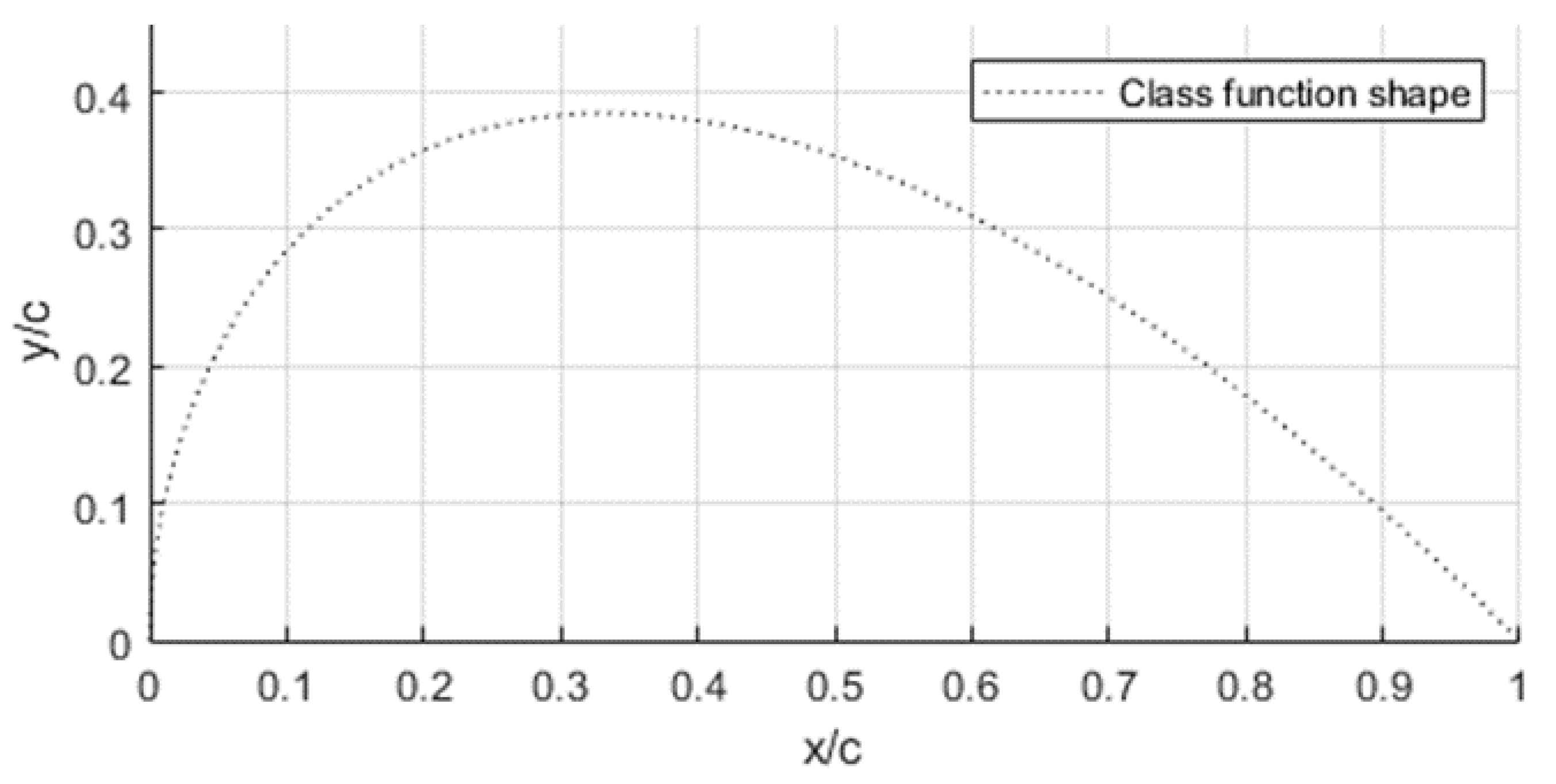
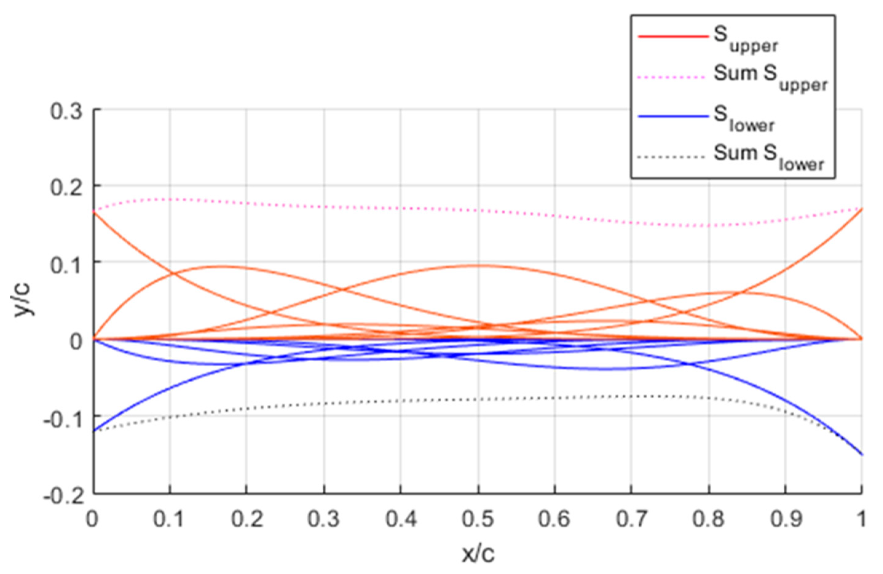
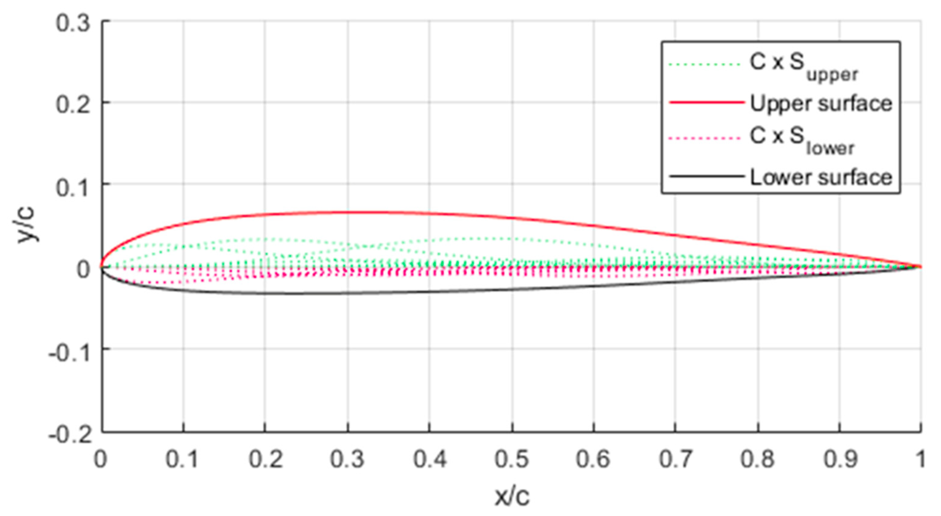
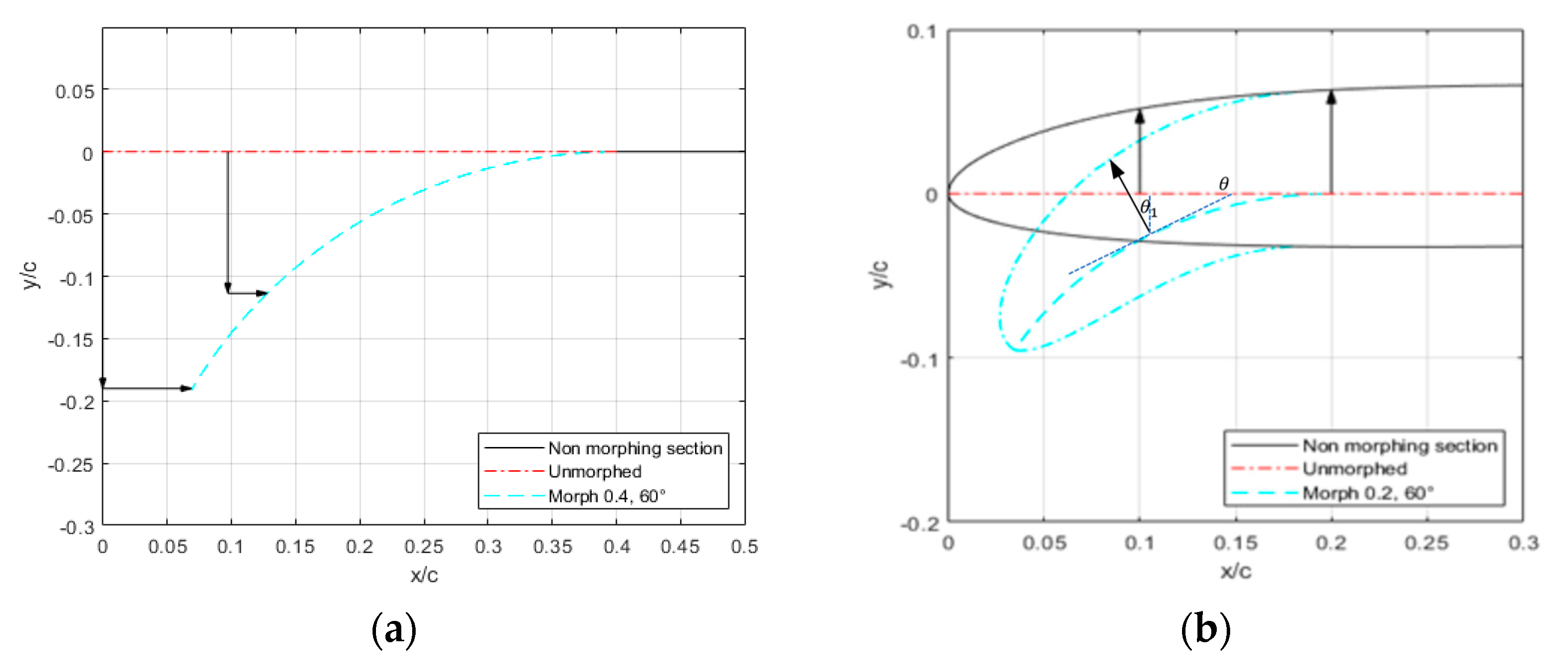
3.1. CST Airfoil Parameterization

The airfoil parameterization is based on a modified class-shape transformation (CST) method, whose equations are based on Kulfan’s [56] work. First, the generalized CST equations are described as they are applied to the airfoil. Next, the upper and lower surfaces of y coordinates are defined individually, using a class function $C\left(\frac{x}{c}\right)$ and a shape function $S\left(\frac{x}{c}\right)$.

$$y_{upper}=C_{N_2}^{N_1}\left(\frac{x}{c}\right)S_{upper}\left(\frac{x}{c}\right)+y_{upperLE}\left(\frac{x}{c}\right)$$

(1)

$$y_{lower}=C_{N_2}^{N_1}\left(\frac{x}{c}\right)S_{lower}\left(\frac{x}{c}\right)+y_{lowerLE}\left(\frac{x}{c}\right)$$

(2)

where $\frac{x}{c}$ and $\frac{y}{c}$ are defined in percentage of the chord of the aircraft (therefore, $\frac{x}{c}$ has a value between 0 and 1) and $N_1$ and $N_2$ are 0.5 and 1, respectively.

The class function is defined as in Equation (3):

$$C_{N_2}^{N_1}\left(\frac{x}{c}\right)={\left(\frac{x}{c}\right)}^{N_1}{\left(1-\frac{x}{c}\right)}^{N_2}$$

(3)

The airfoil given by the class function is a primary airfoil and will be a basis for further airfoils by being multiplied by the value of the shape function. The class function values are shown in Figure 3.

The shape functions produce the specific shapes of the airfoil. The function is composed of various weights $W_{upper}\left(i\right)$ and $W_{lower}\left(i\right)$ defined as a real value, and is dependent of i, inside a Bernstein polynomial [55]. The equations for the upper and lower surfaces differ;

$$S_{upper}\left(\frac{x}{c}\right)={\displaystyle \sum }_{i=0}^{N_{upper}}{S}_{upper}\left(\frac{x}{c}, i\right)={\displaystyle \sum }_{i=0}^{N_{upper}}{W}_{upper}\left(i\right) B_{upper}$$

(4)

$$S_{lower}\left(\frac{x}{c}\right)={\displaystyle \sum }_{i=0}^{N_{lower}}{S}_{lower}\left(\frac{x}{c}, i\right)={\displaystyle \sum }_{i=0}^{N_{lower}}{W}_{lower}\left(i\right) B_{lower}$$

(5)

where

$$B_{upper}=K_i^{N_{upper}} {\left(\frac{x}{c}\right)}^i {\left(1-\frac{x}{c}\right)}^{N_{upper}-i}$$

(6)

and

$$B_{lower}=K_i^{N_{lower}} {\left(\frac{x}{c}\right)}^i {\left(1-\frac{x}{c}\right)}^{N_{lower}-i}$$

(7)

are the Bernstein polynomials, and $K_i^N$ is the binomial coefficient K:

$$K_i^N=\frac{n!}{i!\left(n-i\right)!}$$

(8)

In which i is the value of the Bernstein polynomials’ order.

The following graph shows both each individual S(x, i) value for i, as well as their sum to obtain S(x), when using the weights W(i) for the UAS S-45’s airfoil (Figure 4). Those weights were determined by matching the S-45’s airfoil to the weights that best fit the airfoil using Matlab’s nonlinear programming solver.

When C(x) and S(x) are multiplied, and assuming both $y_{upppe{r}_{LE}}$ and $y_{lowe{r}_{LE}}=0$, the airfoil shapes shown in Figure 5 are obtained.

Most typical CST LE morphing can only occur by adding a y-axis deflection to control points, and may have a constraint to maintain a constant skin length. However, that y-axis deflection neglects the x-axis deflection that occurs in a droop-nose leading-edge morphing.

There is also a need to constrain the droop-nose leading-edge morphing. Therefore, new parameters are added to impose where the deflection of the LE on the wing $\left(Morp{h}_{length}\right)$ begins, as well as to impose a specific deflection angle (θ). The approach taken assumes that there is an axis located on the $\frac{x}{c}$ axis that serves as a basis for the morphing. An arc that is a tangent to the $\frac{x}{c}$ axis on one side and tangent to the deflection angle on the other side begins at $\frac{x}{c}=Morp{h}_{length}$. The length of the arc is that of $Morp{h}_{length}$. The skin keeps its relative position to the closest point on the morphing mechanism, meaning that it keeps the same distance that is perpendicular to the mechanism’s arc. Figure 6 illustrates the setup by showing the axis and arc’s neutral unmorphed position and then its variation of $\frac{y}{c}$ with $\frac{x}{c}$ while morphing occurs. For example, the Morph 0.2, 30° figure’s morphing begins at $\frac{x}{c}=0.2$, and the tangent of the end of the arc that is not on $\frac{y}{c}$ = 0 has a 30° angle to the $\frac{x}{c}$ axis.

To calculate morphing position with the CST parameterization, the morphing process is conducted in two steps; the first process is considering y/c translation, and the second is considering $\frac{x}{c}$ translation. The translation itself is the sum of both the translation from the mechanism and the translation from the skin to the mechanism that is produced by the rotation of the mechanism. Figure 7 depicts the translation, with both axes from the deflection arc and skin movement in relation to the deflection arc. In Figure 7a, the deflection arc begins at $\frac{x}{c}=0.4$, and the tangent to the free end of the arc is 60° from the $\frac{x}{c}$ axis. The movement of the airfoil skin follows the movement of the deflection arc, with both a $\frac{x}{c}$ and $\frac{y}{c}$ translation that follow the relative position on the arc from the unmorphed position. In Figure 7b, the relative skin movement from the arc is illustrated. While in the unmorphed position, the relative skin position is right above the selected $\frac{x}{c}$ axis point, when the arc has an angle with the $\frac{x}{c}$ axis, the relative skin position is changed, and is perpendicular to the tangent of the respective arc position, at the same distance as the respective $\frac{y}{c}$ distance between the relative skin position and $\frac{x}{c}$ axis. This translation will be most prominent when the difference between the $\frac{x}{c}$ axis and relative skin position is farther on the unmorphed airfoil, and when the angle between the tangent of the arc and the $\frac{x}{c}$ axis is higher. When $\frac{x}{c}=Morp{h}_{length}$, there is no difference in relative skin position since the tangent of the arc is 0°. When the unmorphed $\frac{x}{c}=0$, there is no relative skin position difference since the distance between the relative skin position and $\frac{x}{c}$ axis is 0 since it is the tip of the leading edge.

The equation to determine the arc center is:

$${\left(\frac{x}{c}-{\frac{x}{c}}_{arc}\right)}^2+{\left(\frac{y}{c}-{\frac{y}{c}}_{arc}\right)}^2={\frac{y}{c}}_{arc}^2$$

(9)

where ${\frac{x}{c}}_{arc}$ and ${\frac{y}{c}}_{arc}$ are the center position of the arc, and assuming ${\frac{y}{c}}_{arc}$ is the radius of the arc, and when using the fact that the center of rotation will be just under the beginning of the morphing section and that we know the position at which the morphing begins, we use

$${\frac{x}{c}}_{arc}=Morp{h}_{length}$$

(10)

so that the values for x/c and y/c can be calculated when ${\frac{y}{c}}_{arc}$ is known.

Since we can also know the arc length, as its value is Morph_length, it is possible to determine any other point on the arc. The Θ value is the same as the arc angle value. Therefore, since

$$Arclength=\Theta \ast r$$

(11)

$$Morp{h}_{length}=Arclength$$

(12)

$${\frac{y}{c}}_{arc}=r$$

(13)

$${\frac{y}{c}}_{arc}=\frac{Morp{h}_{length}}{\Theta }$$

(14)

Now the values of any $\left({\frac{x}{c}}_{arc},{\frac{y}{c}}_{arc} \right)$ point coordinates can be determined. The arc lengths $\left(arcl\right)$ from the $Morp{h}_{length}$ position needed to obtain the angle of the morphing section are used to determine the $\frac{x}{c}$ and $\frac{y}{c}$ translared.

Since each skin section is attached to the closest section of the $\frac{x}{c}$ axis, it can be assumed that if the skin position is ${\frac{x}{c}}_{skin}$ and ${\frac{y}{c}}_{skin}$, and so the closest distance between the skin and the $\frac{x}{c}$ axis, $y_{dist}$ is given as:

$${\frac{x}{c}}_{trans}={\frac{x}{c}}_{trans1}+{\frac{x}{c}}_{trans2}$$

(15)

$${\frac{y}{c}}_{trans}={\frac{y}{c}}_{trans1}+{\frac{y}{c}}_{trans2}$$

(16)

where $x_{trans1}$, $x_{trans2}$, $y_{trans1}$, and $y_{trans2}$ are the respective $\frac{x}{c}$ and $\frac{y}{c}$ translation from the deflection arc (1) and the relative skin movement in relation to the arc (2) which are included independently to the upper and lower surfaces. Finally, the following equation is obtained:

$$y_{upper}=C_{N_2}^{N_1} \left(\frac{x}{c}\right) S_{upper} \left(\frac{x}{c}\right)+y_{trans upper} \left(\frac{x}{c}\right)|\frac{x}{c}<Morp{h}_{length}$$

(17)

$$y_{lower}=C_{N_2}^{N_1} \left(\frac{x}{c}\right) S_{lower}\left(\frac{x}{c}\right)+y_{trans lower} \left(\frac{x}{c}\right)|\frac{x}{c}<Morp{h}_{length}$$

(18)

$$y_{upper}=C_{N_2}^{N_1}\left(\frac{x}{c}\right)S_{upper}\left(\frac{x}{c}\right)|\frac{x}{c}\ge Morp{h}_{length}$$

(19)

$$y_{lower}=C_{N_2}^{N_1}\left(\frac{x}{c}\right)S_{lower}\left(\frac{x}{c}\right)|\frac{x}{c}\ge Morp{h}_{length}$$

(20)

To translate the x, the function is no longer a function of $\frac{x}{c}$ but instead a function of $\frac{x}{c}-x_{trans}\left(\frac{x}{c}\right)$ while $\frac{x}{c}<Morp{h}_{length}$ for a fixed $\Theta$ and a fixed $Morp{h}_{length}$.

$$y_{upper}=C_{N_2}^{N_1}\left(\frac{x}{c}-X_{tu}\right)S_{upper} \left(\frac{x}{c}-X_{tu} \right)+y_{trans upper}\left(\frac{x}{c}-X_{tu}\right)|\frac{x}{c}-X_{tu}<Morph\_length$$

(21)

$$y_{lower}=C_{N_2}^{N_1}\left(\frac{x}{c}-X_{tl}\right)S_{lower} \left(\frac{x}{c}-X_{tl} \right)+y_{trans lower} \left(\frac{x}{c}-X_{tl} \right)|\frac{x}{c}-X_{tl }<Morp{h}_{length}$$

(22)

where

$$X_{tu}=x_{trans upper}\left(\frac{x}{c}\right)$$

(23)

$$X_{tl}=x_{trans lower}\left(\frac{x}{c}\right)$$

(24)

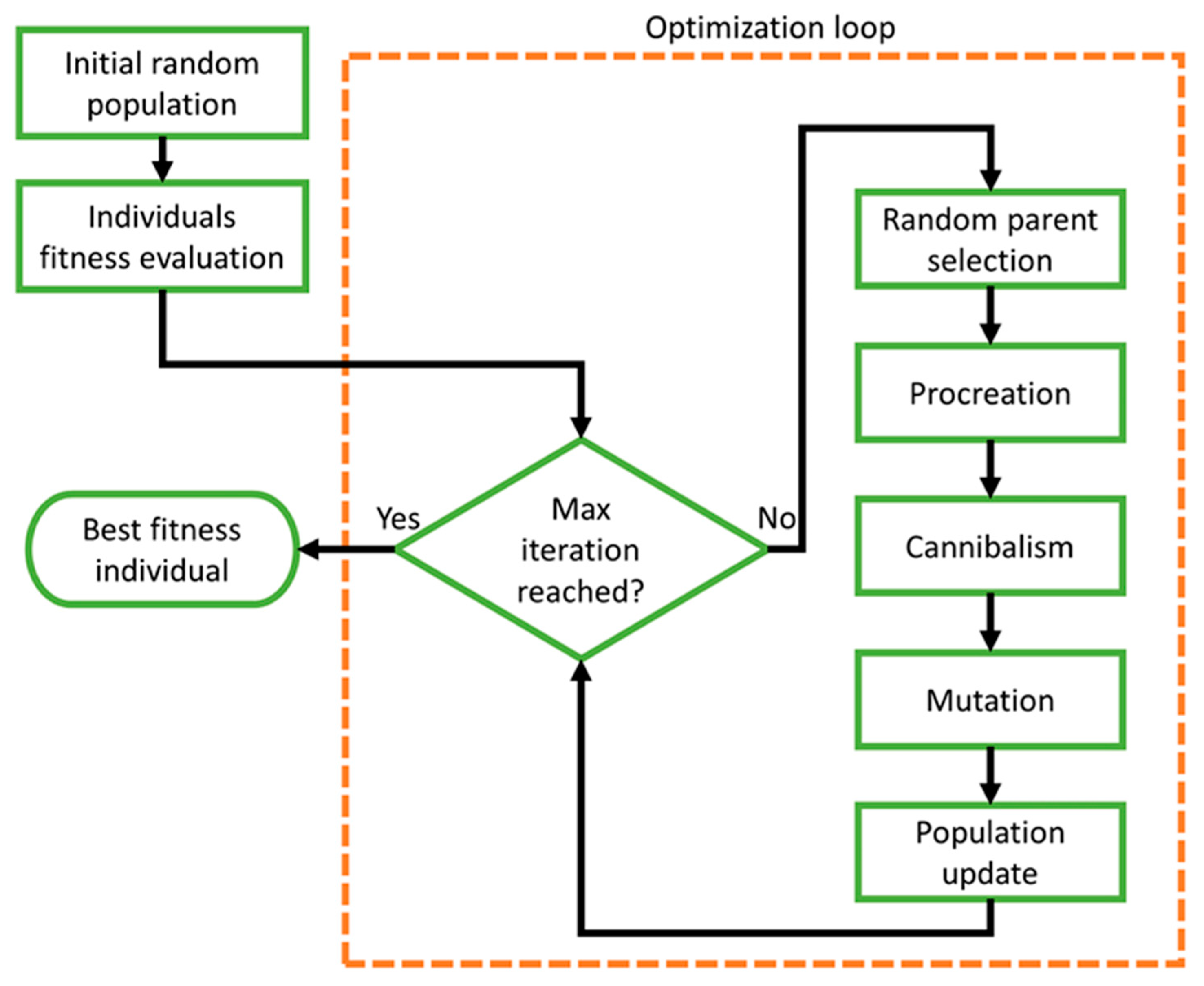
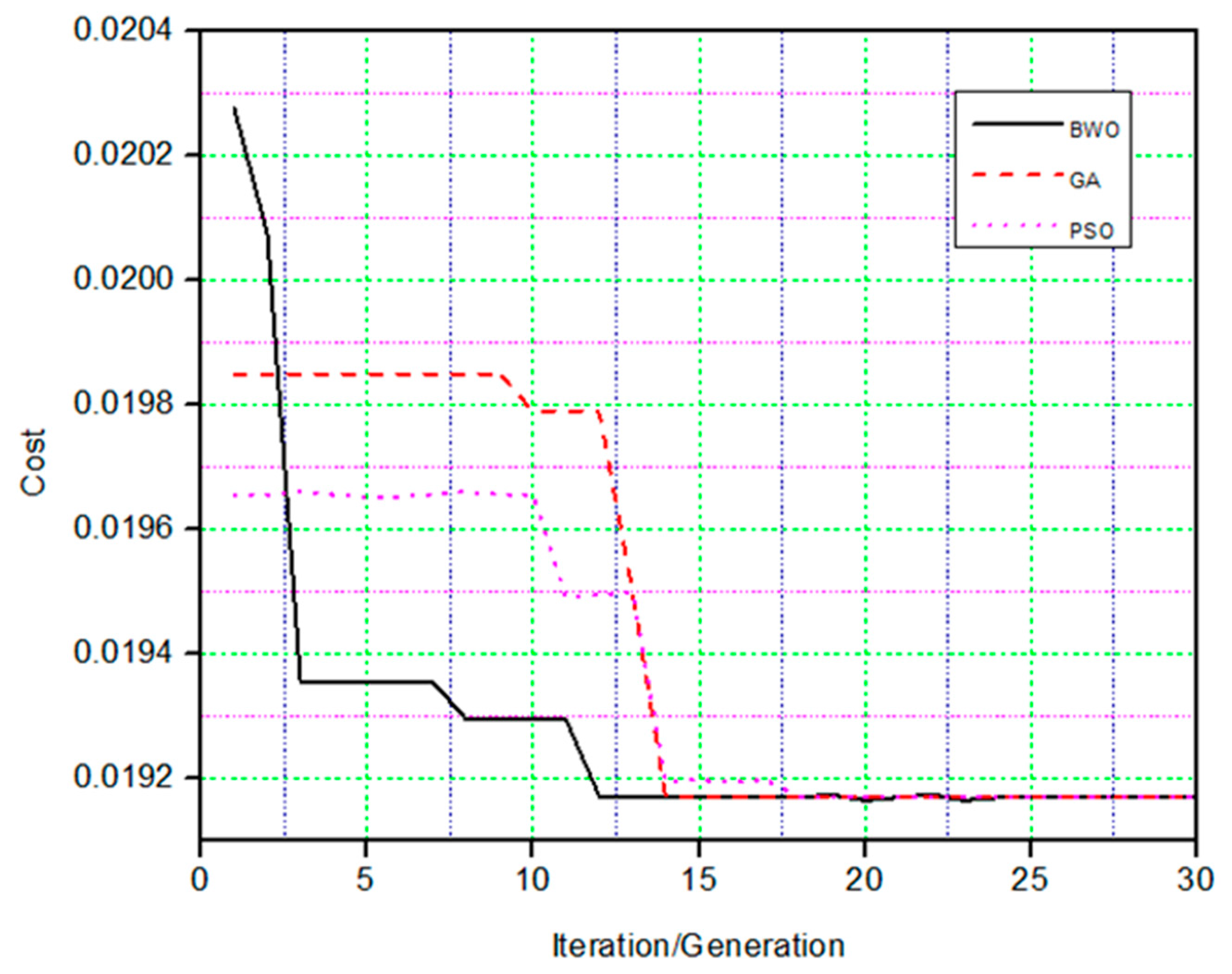
3.2. Black Widow Optimization (BWO)

Several nature-inspired algorithms by biological systems, including particle swarm optimization (PSO), bee colony optimization (BCO), ant colony optimization (ACO), and genetic algorithm (GA) have been used for airfoil optimization [57,58,59]. Each of these methods optimizes globally. Recent work has proposed the use of Black Widow Optimization (BWO) to solve numerical optimization problems [60]. This algorithm was inspired by the black widow spider’s life cycle. The black widow spider is well known for its unusual mating behavior, which served as the inspiration for the algorithm utilized in this study; consider it a combination of evolutionary and swarm techniques. The BWO includes a phase that is unique, called “cannibalism”. This phase has the advantage of excluding species with inadequate fitness from the circle, ensuing in algorithms converging faster. When compared to the other studied algorithms, the suggested BWO algorithm is capable of avoiding local optima. This algorithm makes no use of additional information, such as the objective function’s gradient values.

The BWO algorithm is well known for its staged implementation (Procreation, Cannibalism, and Mutation), as well as its various parameters such as procreating rate, cannibalism rate, and mutation rate. The more these parameters alter, the greater the possibility of jumping out of a local optimum, and thus the greater the ability to explore the search space globally. This results in the equilibrium of these two stages of exploitation and exploration. This Procreation option can be used to regulate the transition of search agents from the global stage to the local stage, as well as to direct them toward the optimal solution. According to the literature, the procreation step aids the BWO algorithm solution in overcoming local optima by utilizing a large number of search agents to attain the global optima [60].

Black Widow Optimization (BWO) is a fascinating biomimetic for resolving difficult numerical optimization problems [60]. BWO, as with other evolutionary algorithms, incorporates conditions that emulate natural evolutionary processes such as selection, reproduction, and mutation. The flowchart in Figure 8 illustrates the BWO’s primary steps in a concise manner.

The following are brief summaries of the BWO’s primary steps:

In the initial population phase, each spider represents a potential solution. These initial spiders, in pairs, try to reproduce the new generation. The female black widow eats the male during or after mating. This section of the population can be defined as follows:

$$widow=\left(y_1, y_2,\dots , yPo{p}_{var}\right)$$

(25)

where $Po{p}_{var}$ is the optimization problem’s dimension. $Po{p}_{var}$ is also the number of threshold values the algorithm must obtain. Each set’s fitness function f determines a widow’s fitness given by $\left(y, y_2, \dots , yPo{p}_{var}\right)$. The widow fitness f(widow) can thus be written as:

$$Fitness=f\left(widow\right)=f \left(y_1, y_2,\dots , y{P}_{var}\right)$$

(26)

The initial spider population is used with the candidate matrix $\left(M_{pop}\times M_{var}\right)$.

In the Procreation stage, each pair mates in its own web, independently of the others. In reality, each pairing produces around 1000 eggs, but only a few of the spider infants survive. If an array called gamma contains random numbers, then children are formed by utilizing the following Equations (27) and (28), and the offspring is formed.

$$x_1=\gamma \times y_1 +\left(1-\gamma \right)\times y_2$$

(27)

$$x_2=\gamma \times y_2 +\left(1-\gamma \right)\times y_1$$

(28)

where the parents are denoted by $y_1$ and $y_2$ and the offspring by $x_1$ and $x_2$. The process is reiterated $Po{p}_{var}$ times. The fitness value is stored by adding the parents and offspring. A cannibalism rating (CR) according to which the number of survivors is determined is set. Based on the CR, some of the best individuals are added to the newly created population.

In Cannibalism, there are three types: sexual, sibling, and cannibalism, where newborn spiders eat their mothers. This process is then analyzed and documented in proportion to the number of survivors, yielding a cannibalism rating. These fitness ratings help distinguish weak from robust offspring.

In the Mutation stage, the population is randomly picked from the population to be mutated throughout the mutation process. Each of the chosen solutions randomly flips two elements of the array. By integrating all populations, the new population is evaluated and stored. This procedure is used to determine the matrix’s optimal widow.

Figure 9 illustrates the convergence plots of the cost function versus the number of iterations for the GA, PSO, and BWO algorithms. According to the convergence plot obtained from optimizing an airfoil for drag minimization at the same flight conditions and design variables for all these algorithms, The GA method requires 14 iterations to attain the global minimum value of 0.019, the PSO algorithm requires 18 iterations, and the BWO algorithm requires only 11 iterations. As a result, the BWO algorithm surpassed the GA and PSO algorithms in terms of performance.

3.3. Aerodynamic Solver

The aerodynamic solver is used to evaluate the performance of airfoil geometry in terms of aerodynamics. For evaluating aerodynamic performance, this study used two solvers, XFoil and Ansys Fluent. The selection of a turbulence model, the grid convergence for the mesh topology, and size were all part of the validation process.

3.3.1. XFoil Solver

External aerodynamics problems benefit significantly from panel approaches, which are based on the velocity potential flow theory. Panel methods result in reliable pressure and velocity distributions along an airfoil with little computational expense when the linearization hypothesis is valid. The velocity field can be represented as the gradient of a scalar potential. Linear methods can be used on thin bodies at modest angles of attack when there is no extensive separation, and the regime is subsonic. Drela’s XFoil [51] is a popular program that predicts fixed or free transitions, mild trailing-edge separation, and lift and drag prediction using linear flow and a viscous boundary-layer (BL) interaction.

XFoil has difficulty providing a convergent solution for the airfoil analysis at high angles of attack where stall develops. To ensure solution convergence, non-converged explanations are penalized heavily by arbitrarily increasing the fitness function via a penalty function. As a result, they are finally omitted from the design process.

The findings obtained with XFoil were compared to those obtained with experimental data or with high-fidelity solvers, and only a tiny difference was noted [61].

3.3.2. Transition SST Model

Aerodynamic data prediction needs precise recirculation of pressure drops, computation of boundary layers, and flow separation. While some studies incorporate the wall function of the flow model within the boundary layer into the RANS turbulence model, this sort of turbulent model is insufficient for effectively predicting the boundary layer, flow maintenance, pressure drop, and flow separation. Due to the fact that direct numerical simulations (DNSs) and other eddy-resolved simulations are all extremely high computational techniques, the numerical analysis utilized the Transition SST turbulence model to generate highly precise and computationally efficient aerodynamic data.

The Transition $\left(\gamma -R{e}_{\theta }\right)$ SST was employed in this investigation. This model uses SST K-ω, intermittency, and a transition onset Reynolds number. $\left(\gamma -R{e}_{\theta }\right)$ is the crucial Reynolds number [62]. The intermittency of the boundary-layer transition activates the turbulent kinetic energy generation term. Unlike the more usual use of intermittency to vary eddy viscosity, this method simulates higher laminar skin friction by modeling high freestream turbulence on laminar boundary layers. The fourth transport equation for Re is required for non-local turbulence strength. The additional transport equation also allows for numerous possibilities for different boundary conditions, creating a versatile and flexible tool.

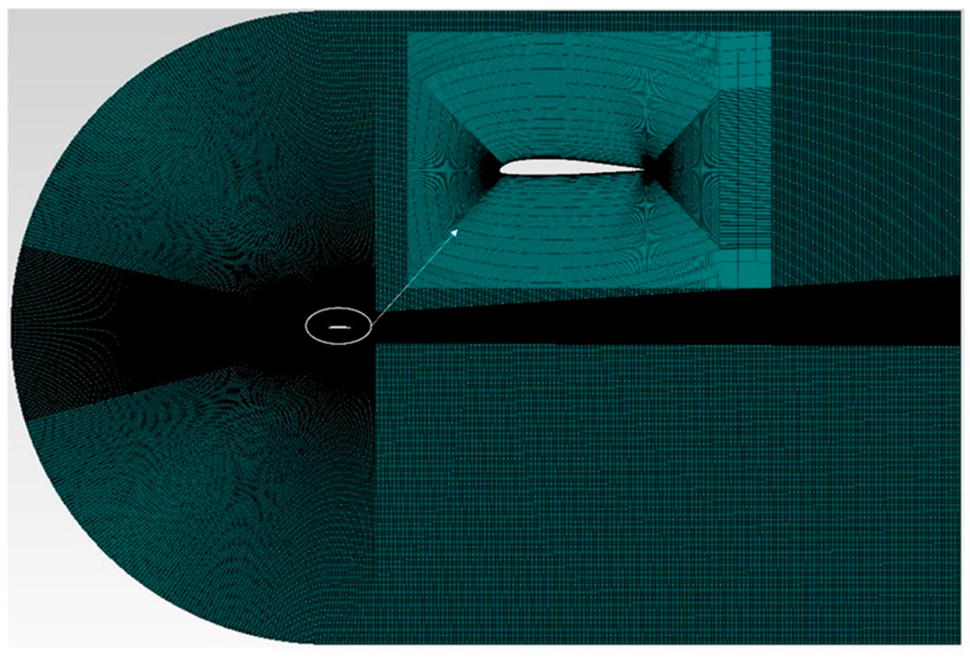
3.3.3. Mesh Generation

ICEM was used to discretize the computational domain and solve each node using the governing equation. The airfoil geometries defined the C-shaped computational domain. The outlet boundary was established at 30 c (c being the chord length) to agree for the full development of the wake flow. The distance was selected at 10 c to prevent altering the flow field upstream of the airfoil. The dense grids formed in the airfoil’s boundary layer, with smaller grid cells as they moved away from the surface. Laminar and transitional boundary layers can be captured using beginning layer thickness. Mesh topology surrounding the computational domain is shown in Figure 10.

The intake was set at 34 m/s with a turbulence rate of 0.01 percent. The airfoil’s surface was made non-slip and smooth. The outlet had a static gauge pressure of zero. The iterations ended when all scaled residuals were less than 1 × 10⁶.

The grid independence investigation was performed by altering the number of nodes in the dense mesh region. The drag coefficient was chosen as the mesh dependency criterion. Grid sizes of 100, 200, and 300 nodes were adequate to collect the results. The mesh size was then increased until additional increases in the mesh yielded very little difference in the values of drag coefficient.

4. Results and Discussion

The optimization results from coupling the CST parameterization methods with the Black Widow Optimization (BWO) algorithm for the UAS-S45 airfoil for the Droop-Nose Leading-Edge (DNLE) Morphing design were obtained. DNLE configurations consist of the focus of this research. A reference airfoil shape optimization was performed to fully influence the “morphing” concept, followed by its morphing airfoil shape design. These scenarios are based on different altitudes and Reynolds numbers calculated for a 34 m/s airspeed, which were chosen because the UAS-S45 can reach altitude of 20,000 ft and has a stall speed of 34 m/s. The endurance maximization was chosen as an optimization function to improve the performance of the UAS-S45 over a large part of its flying regimes.

4.1. Optimization of Cruise Phase

The cruise flight condition was chosen because most of the flight time and fuel consumption occurs during the cruise phase. Accordingly, the objective functions were selected to maximize the aerodynamic endurance and to minimize the drag. The maximum lift coefficient and the lift coefficient of the reference airfoil at each angle of attack were implemented as constraints. Penalty functions applied constraints to the objective function to ensure that the optimum performance was obtained at each given angle of attack. The free-stream Mach number was 0.1, and the Reynolds number was 2.4 × 10⁶. The general optimization problem is presented as follows:

The mathematical formulation of the drag minimization objective function is the following.

$$\mathrm{Minimize}{C}_D \left(x\right);x ϵ \left(airfoil set\right)$$

(29)

$$\mathrm{subject}\mathrm{to}{C}_{L_{max}}\left(x, \alpha , M \ge \right)1.608$$

$$C_{L_{morph}}\ge C_{L_{min,baseline}\left(x,\alpha ,M\right)}\left(x\right);xϵairfoilset$$

For the design of a long endurance UAV, the aerodynamic endurance (E) of a propeller-powered UAV, as established by using the Breguet formula [63], is used as an objective function:

$$\mathrm{Minimize}{E}_a\left(x\right)=\frac{C_L^{\frac{3}{2}}}{C_D};x ϵ \left(airfoil set\right)$$

(30)

$$\mathrm{subject}\mathrm{to}{C}_{L_{max}}\left(x, \alpha , M \ge \right)1.608$$

$$C_{L_{morph}}\ge C_{L_{min,baseline}\left(x,\alpha ,M\right)}\left(x\right);xϵairfoilset$$

4.1.1. Drag Minimization

Drag minimization is achieved by optimizing the shape of a morphing Droop-Nose Leading Edge (DNLE) to increase aerodynamic efficiency during the cruise. The morphing location is kept as a variable and leading-edge morphing takes place within 30% chord to ensure that the rest of the airfoil remains as a wing box without any changes. The performances of the reference and optimized airfoils are compared and presented in

Table 1. Comparison of aerodynamic coefficients of the reference and optimized.

	Angle of Attack (°)	Reference Airfoil	Optimized Airfoil	Relative Difference in ‘%’
$C_D$	2°	0.00755	0.00663	−12
$\frac{C_L}{C_D}$	2°	48.6887	56.1017	15

. The drag coefficient reduces to 0.00678, with 12% versus its initial value. An aerodynamic efficiency improvement of 15% is achieved by optimizing the lift-to-drag ratio.

Figure 11a illustrates the initial (reference) versus the final (optimized or morphed) DNLE airfoil shape. Figure 11b shows the pressure coefficient calculated for the minimum drag-optimized airfoil at an angle of attack of 2° versus its reference airfoil. A less unfavorable pressure gradient and smoother pressure peak than the original airfoil allows for longer laminar flow. Figure 11 compares the pressure coefficient fluctuations of optimized and reference airfoils with the chord (b). Pressure changes on the pressure side of the airfoil for a 2° angle of attack show the flow transition. By delaying turbulent flow towards the trailing edge, the DNLE optimized airfoil cruises better.

Figure 12a,b shows the pressure contours over the upper and lower surfaces of the reference and optimized airfoils at an angle of attack of 2°. The DNLE creates more negative pressure as seen in Figure 12b than the baseline airfoil in Figure 12a. Hence, more lift was generated in the optimized airfoil.

The optimized airfoil’s skin friction coefficient shows that the laminar-to-turbulent transition area is delayed by almost 10% of the chord, from 25% to 35% for the original airfoil, as shown in Figure 13. Increasing the angle of attack reduces the drag coefficient by increasing laminar flow and decreasing pressure drag.

Figure 14a shows the chordwise fluctuations of velocity magnitude contours at a 2° angle of attack. The lower surfaces of the reference and optimized airfoils have marginally lower velocities than the higher surfaces. The location of the airfoil’s stagnation points changed between the optimized and reference airfoils. In Figure 14b, turbulence causes the intermittency factor to rapidly develop. As mentioned in Section 3.3.2, on the upper surface, the intermittency rapidly increases from 0 to 1, showing the transition starting point. The beginning of the transition can be seen as an increase in intermittency near the surface, which then grows to unity at a certain distance. The intermittency’s production is delayed in the optimized airfoil as compared to the baseline airfoil. The flow on the upper surface is laminar, but it reattaches and transforms into a turbulent flow.

Table 2. Optimized drag results for the reference and optimized morphing airfoils for a certain length of a flexible morphing section for drag minimization.

Angle of Attack	Length of Flexible Section (m)	Reference Airfoil C_D	Optimized Airfoil C_D	Relative ‘%’ Difference
0	0.05	0.0091	0.00691	−24.06
1	0.10	0.00801	0.00729	−8.98
2	0.07	0.00755	0.00663	−12.18
3	0.09	0.0093	0.00674	−27.52
4	0.23	0.00976	0.00643	−34.11
5	0.24	0.0102	0.00648	−36.47
6	0.23	0.00912	0.00678	−25.65
7	0.29	0.01016	0.0097	−4.52
8	0.29	0.01261	0.01143	−9.35
9	0.25	0.01251	0.01108	−11.43
10	0.29	0.01386	0.0129	−6.92

presents a comparison between the drag coefficients for the reference airfoil and the optimized morphing airfoil. The drag coefficient reduction of the morphing optimized airfoil over the original reference airfoil was obtained for the range of angles of attack from 0° to 10°. At each angle of attack, the relative error describing the drag reduction is indicated. The best improvements in the drag reduction were found for the angle of attack between 2° and 6°.

The drag minimization optimization increased the lift-to-drag ratio, as the lift coefficients remain relatively the same for the reference airfoil and the optimized airfoil. Figure 15 shows the lift-to-drag coefficient increments for the given drag coefficients for the optimized airfoil as compared to the original airfoil coefficients, for the Reynolds number of 2.4 × 10⁶.

4.1.2. Endurance Maximization

Another optimization case concerns optimizing the shape of an airfoil-morphing Droop-Nose Leading Edge (DNLE) with respect to the reference leading edge in order to increase aerodynamic efficiency during the cruise phase by maximizing its aerodynamic endurance.

Table 3. Comparison of aerodynamic endurance and minimized drag of the reference and optimized airfoils.

	Reference Airfoil	Optimized Airfoil	Relative Difference in ‘%’
$\frac{\left(C_L^{\frac{3}{2}}\right)}{C_D}$	29.52	32.48	10
$C_D$	0.00872	0.00796	−8

shows that the optimization process led to an increase in endurance maximization, characterized by $\frac{C{L}^{\frac{3}{2}}}{CD}$ in the optimized DNLE airfoil. Furthermore, the values of $\frac{C{L}^{\frac{3}{2}}}{CD}$ increased from 29.52 to 32.48, indicating a 10% better endurance performance for the UAS-S45 DNLE airfoil configurations than that of the reference airfoil. At the same time, the drag coefficient for the optimized airfoil was smaller than CD obtained for the reference airfoil.

Figure 16a illustrates the initial (reference) versus the final (optimized or morphed) airfoil shape, while Figure 16b shows the pressure coefficients for the minimum drag optimized airfoil and the reference airfoil at an angle of attack of 2°. The change in the leading-edge shape of the optimized airfoil as compared to the reference airfoil is obtained by extending the flexible leading-edge section in the optimized airfoil. The optimized leading-edge deflection slightly drops around 12.58°. Similarly, on Figure 16b, it can be observed that the optimized airfoil presents a smoother pressure peak and that the adverse pressure gradient is not as strong as the original airfoil pressure gradient, thus creating favorable conditions for an extended laminar flow. The pressure-value variations with the chords of the optimized airfoils versus the reference airfoil are shown in Figure 16c. It is clear that the most significant pressure fluctuations occur around the leading edge’s upper surface. The chord-wise pressure distribution indicates the increased performance for the DNLE optimized airfoil at the cruise phase achieved by delaying the onset of turbulent flow towards the trailing edge.

The skin friction coefficient in Figure 17 shows that the laminar-to-turbulent transition zone is delayed by almost 10% of the chord, from 25% to 35% in the original airfoil. As the angle of attack increases, the laminar flow extent increases while the pressure drag decreases.

Figure 18a shows the velocity contour plots of one of the DNLE airfoils for a 2° angle of attack. Comparing the reference and DNLE airfoils reveals that the DNLE airfoil has higher gradients than the reference airfoil. The improved airfoil’s stagnation points were different. The improved airfoil showed a 15% increase in lift-to-drag coefficient ratio compared to the reference airfoil. Figure 18b shows the separation-induced transition where turbulence rapidly increases the intermittency factor. The beginning of the transition can be seen as an increase in the intermittency near the surface, which then grows to unity at a certain distance. The intermittency’s production is delayed from 0.3 c in the reference airfoil to 0.37 c in the optimized airfoil. The flow on the airfoil upper surface is laminar, but it reattaches and transforms into a turbulent flow.

Table 4. Optimized drag results for the reference and optimized morphing airfoils for a certain length of a flexible morphing section for maximization of endurance.

Angle of Attack (°)	Length of Flexible Section $\left(\frac{\mathit{l}}{\mathit{c}}\right)$	Reference $\frac{{\mathit{C}}_{\mathit{L}}^{\frac{3}{2}}}{{\mathit{C}}_{\mathit{D}}}$	Optimized $\frac{{\mathit{C}}_{\mathit{L}}^{\frac{3}{2}}}{{\mathit{C}}_{\mathit{D}}}$	Improvement ‘%’
0	0.19	5.86	9.06	54.51
1	0.06	15.28	19.54	27.86
2	0.12	29.52	32.48	10.05
3	0.06	34.68	49.78	43.55
4	0.24	44.63	65.67	47.13
5	0.18	55.30	93.42	68.94
6	0.21	78.94	114.83	45.45
7	0.19	81.90	130.02	58.75
8	0.22	78.81	142.62	80.96
9	0.23	91.34	154.41	69.05
10	0.20	95.11	160.50	68.74

presents a comparison between the aerodynamic endurance for the reference airfoil and for the optimized airfoil. The increase in the aerodynamic endurance of the optimized airfoil over the original reference airfoil was obtained for the range of angles of attack from 0° to 10°. The improvement percentage is indicated for each angle of attack value.

The complete flight profile of a surveillance-based UAV consists mostly of take-off, climb, cruise, standby, evacuation, return, descent, and landing phases, and engine working states in different flight phases are varied. Therefore, all missions require improved performance, and account for the different flight times and fuel consumption. A Simulink model of UAS-S45 was developed for fuel burn rate and specific fuel consumption in MATLAB, using the coefficient of thrust from both engines, as well as their associated fuel consumption.

The fuel burn rate and specific fuel consumption were obtained for both the reference and optimized aerodynamic coefficients when the drag of the aircraft was equal to the thrust (in equilibrium uniform flight). A relationship between the lift and drag coefficients at various angles of attack was used to determine the drag for the weight of the aircraft in order to match the corresponding lift. The drag and lift were obtained from their corresponding aerodynamic coefficients using the following equations:

$$Lift=\frac{1}{2}\ast \rho \ast v^2\ast S\ast CL$$

(31)

$$Drag=\frac{1}{2}\ast \rho \ast v^2\ast S\ast CD$$

(32)

where $\rho$ is the air density, v is the airspeed, S is the wing surface (assumed to remain same), and CL and CD are the lift and drag coefficients, respectively.

Figure 19a–d shows the DNLE morphing airfoil fuel burn for three different optimization functions expressed in terms of drag minimization Figure 19b, lift-to-drag maximization Figure 19c, and aerodynamic endurance maximization Figure 19d as compared to baseline Figure 19a, and all of them indicate that the fuel consumption was reduced with respect to the reference airfoil. Figure 20a–d shows the same results for the specific fuel consumption.

5. Conclusions

This work performed aerodynamic optimization of Droop-Nose Leading-Edge (DNLE) morphing airfoils for UAS-S45 at cruise flight conditions. A Black Widow Optimization (BWO) algorithm was coupled with a modified Class-Shape Transformation (CST) parameterization method, and was then employed to optimize the aerodynamic shape of a well-known UAS-S45 airfoil, in order to improve its drag and aerodynamic endurance performances. The CST parameterization technique was used to parameterize the reference airfoil by introducing local shape changes and providing skin length control to obtain its various optimized DNLE configurations. These included an in-house MATLAB method, an aerodynamic solver, and a high-fidelity CFD solver. Validity was assessed for both options. It was predicted by Transition $\left(\gamma -R{e}_{\theta }\right)$ SST turbulence model.

The DNLE optimization was designed to increase the aerodynamic performance of the UAS-S45 at the cruise phase for an angle of attack of 2°. The DNLE optimized airfoil showed that the drag coefficient reduced to 0.00678, with a 12.18% drag reduction in comparison to the reference airfoil. In addition, an aerodynamic efficiency improvement of up to 15.22% was achieved by increasing lift-to-drag ratio for the optimized UAS-S45 airfoil. A transition onset delay was also observed using the skin friction coefficients on the optimized DNLE airfoils. For the aerodynamic endurance objective function, the values of CL3/2/CD increased from 29.52 to 32.48, thus indicating a 10% better endurance performance for the UAS-S45 optimized airfoil configurations than for its reference airfoil. At the same time, the drag coefficient obtained using the aerodynamic endurance maximization objective function is reduced for the optimized airfoil as compared to the reference airfoil. In addition, it was observed that the DNLE morphing design will result in better fuel consumption when compared to the reference UAV.

In forthcoming work, this morphing optimization study will include the unsteady flow analysis on the DNLE airfoil. The transient behavior of the DNLE airfoil will be presented via a three-dimensional analysis of the UAS-S45 wing with DNLE. Based on aero-structural studies, various configurations will be analyzed, and the actuation mechanism shown in Figure 1 will be implemented.

References

1. Overton, J. Fact Sheet|The Growth in Greenhouse Gas Emissions from Commercial Aviation, Part 1 of a Series on Airlines and Climate Change. 2019. Available online: https://www.eesi.org/papers/view/fact-sheet-the-growth-in-greenhouse-gas-emissions-from-commercial-aviation (accessed on 22 December 2021).
2. Botez, R. Morphing wing, UAV and aircraft multidisciplinary studies at the Laboratory of Applied Research in Active Controls, Avionics and AeroServoElasticity LARCASE. Aerosp. Lab 2018, 1–11. [Google Scholar] [CrossRef]
3. Hamy, A.; Murrieta-Mendoza, A.; Botez, R. Flight Trajectory Optimization to Reduce Fuel Burn and Polluting Emissions Using a Performance Database and Ant Colony Optimization Algorithm; AEGATS ‘16 Advanced Aircraft Efficiency in a Global Air Transport System: Paris, France, 2016. [Google Scholar]
4. Patrón, R.S.F.; Berrou, Y.; Botez, R. Climb, cruise and descent 3D trajectory optimization algorithm for a flight management system. In Proceedings of the AIAA/3AF Aircraft Noise and Emissions Reduction Symposium, Atlanta, GA, USA, 16–20 June 2014; p. 3018. [Google Scholar]
5. Bashir, M.; Longtin-Martel, S.; Botez, R.M.; Wong, T. Aerodynamic Design Optimization of a Morphing Leading Edge and Trailing Edge Airfoil-Application on the UAS-S45. Appl. Sci. 2021, 11, 1664. [Google Scholar] [CrossRef]
6. Khan, S.; Grigorie, T.; Botez, R.; Mamou, M.; Mébarki, Y. Novel morphing wing actuator control-based Particle Swarm Optimisation. Aeronaut. J. 2020, 124, 55–75. [Google Scholar] [CrossRef]
7. Dancila, B.; Botez, R.; Labour, D. Altitude optimization algorithm for cruise, constant speed and level flight segments. In Proceedings of the AIAA Guidance, Navigation, and Control Conference, Minneapolis, MN, USA, 13–16 August 2012; p. 4772. [Google Scholar]
8. Wölcken, P.C.; Papadopoulos, M. Smart intelligent aircraft structures (SARISTU). In Proceedings of the Final Project Conference; Springer: Berlin/Heidelberg, Germany, 2015. [Google Scholar]
9. Noviello, M.C.; Dimino, I.; Amoroso, F.; Pecora, R. Aeroelastic Assessments and Functional Hazard Analysis of a Regional Aircraft Equipped with Morphing Winglets. Aerospace 2019, 6, 104. [Google Scholar] [CrossRef] [Green Version]
10. Dimino, I.; Pecora, R.; Arena, M. Aircraft morphing systems: Elasticity of selected components and modelling issues. In Proceedings of the Active and Passive Smart Structures and Integrated Systems IX, Online. 22 April–9 May 2020; p. 113760M. Available online: https://www.researchgate.net/publication/341504684_Aircraft_morphing_systems_elasticity_of_selected_components_and_modelling_issues (accessed on 22 December 2021).
11. Ameduri, S.; Concilio, A. Morphing wings review aims, challenges, and current open issues of a technology. Proc. Inst. Mech. Eng. Part C J. Mech. Eng. Sci. 2020. [Google Scholar] [CrossRef]
12. Botez, R.M.; Molaret, P.; Laurendeau, E. Laminar flow control on a research wing project presentation covering a three-year period. In Proceedings of the 2007 Canadian Aeronautics and Space Institute Annual General Meeting, Toronto, ON, Canada, 24–27 April 2007; 2007. Available online: https://www.researchgate.net/profile/Ruxandra-Botez/publication/270396714_Laminar_Flow_Control_on_a_Research_Wing_-_Project_Presentation_on_a_Three-Year_Period/links/54aa09440cf2eecc56e6c989/Laminar-Flow-Control-on-a-Research-Wing-Project-Presentation-on-a-Three-Year-Period.pdf (accessed on 22 December 2021).
13. Communier, D.; Botez, R.M.; Wong, T. Design and Validation of a New Morphing Camber System by Testing in the Price-Païdoussis Subsonic Wind Tunnel. Aerospace 2020, 7, 23. [Google Scholar] [CrossRef] [Green Version]
14. Barbarino, S.; Bilgen, O.; Ajaj, R.M.; Friswell, M.I.; Inman, D.J. A review of morphing aircraft. J. Intell. Mater. Syst. Struct. 2011, 22, 823–877. [Google Scholar] [CrossRef]
15. Sugar-Gabor, O.; Koreanschi, A.; Botez, R.M.; Mamou, M.; Mebarki, Y. Analysis of the aerodynamic performance of a morphing wing-tip demonstrator using a novel nonlinear vortex lattice method. In Proceedings of the 34th AIAA Applied Aerodynamics Conference, Washington, DC, USA, 13–17 June 2016; p. 4036. [Google Scholar]
16. Marino, M.; Sabatini, R. Advanced lightweight aircraft design configurations for green operations. In Proceedings of the Practical Responses to Climate Change Conference, Melbourne, Australia, 29 September–1 October 2014; p. 207. [Google Scholar]
17. Eguea, J.P.; da Silva, G.P.G.; Catalano, F.M. Fuel efficiency improvement on a business jet using a camber morphing winglet concept. Aerosp. Sci. Technol. 2020, 96, 105542. [Google Scholar] [CrossRef]
18. Pecora, R. Morphing wing flaps for large civil aircraft: Evolution of a smart technology across the Clean Sky program. Chin. J. Aeronaut. 2021, 34, 13–28. [Google Scholar] [CrossRef]
19. Sodja, J.; Martinez, M.J.; Simpson, J.C.; De Breuker, R. Experimental evaluation of a morphing leading-edge concept. J. Intell. Mater. Syst. Struct. 2019, 30, 2953–2969. [Google Scholar] [CrossRef] [Green Version]
20. Fereidooni, A.; Marchwica, J.; Leung, N.; Mangione, J.; Wickramasinghe, V. Development of a hybrid (rigid-flexible) morphing leading edge equipped with bending and extending capabilities. J. Intell. Mater. Syst. Struct. 2021, 32, 1024–1037. [Google Scholar] [CrossRef]
21. May, M.; Arnold-Keifer, S.; Landersheim, V.; Laveuve, D.; Asins, C.C.; Imbert, M. Bird strike resistance of a CFRP morphing leading edge. Compos. Part C Open Access 2021, 4, 100115. [Google Scholar] [CrossRef]
22. Peter, F.; Lammering, T.; Risse, K.; Franz, K.; Stumpf, E. Economic assessment of morphing leading-edge systems in conceptual aircraft design. In Proceedings of the 51st AIAA Aerospace Sciences Meeting including the New Horizons Forum and Aerospace Exposition, Grapevine, TX, USA, 7–10 January 2013; p. 145. [Google Scholar]
23. Burnazzi, M.; Radespiel, R. Assessment of leading-edge devices for stall delay on an airfoil with active circulation control. CEAS Aeronaut. J. 2014, 5, 359–385. [Google Scholar] [CrossRef]
24. Kintscher, M.; Wiedemann, M.; Monner, H.P.; Heintze, O.; Kühn, T. Design of a smart leading-edge device for low speed wind tunnel tests in the European project SADE. Int. J. Struct. Integr. 2011, 2. [Google Scholar] [CrossRef]
25. Li, Y.; Wang, X.; Zhang, D. Control strategies for aircraft airframe noise reduction. Chin. J. Aeronaut. 2013, 26, 249–260. [Google Scholar] [CrossRef] [Green Version]
26. Moens, F. Augmented aircraft performance with the use of morphing technology for a turboprop regional aircraft wing. Biomimetics 2019, 4, 64. [Google Scholar] [CrossRef] [Green Version]
27. Yu, Y.; Zhigang, W.; Shuaishuai, L. Comparative study of two lay-up sequence dispositions for flexible skin design of morphing leading edge. Chin. J. Aeronaut. 2021, 34, 271–278. [Google Scholar]
28. Malik, S.; Elaggan, E.; Dawson, P.J. Design, Analysis and Fabrication of Morphing Airfoil. In Proceedings of the AIAA Scitech 2021 Forum, Virtual. 11–15, 19–21 January 2021; p. 0352. [Google Scholar]
29. Arena, M.; Concilio, A.; Pecora, R. Aero-servo-elastic design of a morphing wing trailing edge system for enhanced cruise performance. Aerosp. Sci. Technol. 2019, 86, 215–235. [Google Scholar] [CrossRef]
30. Carossa, G.M.; Ricci, S.; De Gaspari, A.; Liauzun, C.; Dumont, A.; Steinbuch, M. Adaptive Trailing Edge: Specifications, Aerodynamics, and Exploitation. In Smart Intelligent Aircraft Structures (SARISTU); Springer: Berlin/Heidelberg, Germany, 2016; pp. 143–158. [Google Scholar]
31. Khurana, M.; Winarto, H.; Sinha, A. Airfoil geometry parameterization through shape optimizer and computational fluid dynamics. In Proceedings of the 46th AIAA Aerospace Sciences Meeting and Exhibit, Reno, NV, USA, 7–10 January 2008; p. 295. [Google Scholar]
32. Trad, M.H.; Segui, M.; Botez, R.M. Airfoils Generation Using Neural Networks, CST Curves and Aerodynamic Coefficients. In Proceedings of the AIAA Aviation 2020 Forum,, Virtual. 15–19 June 2020; p. 2773. [Google Scholar]
33. Vecchia, P.D.; Daniele, E.; D’Amato, E. An airfoil shape optimization technique coupling PARSEC parameterization and evolutionary algorithm. Aerosp. Sci. Technol. 2014, 32, 103–110. [Google Scholar] [CrossRef]
34. Kulfan, B.M. Recent extensions and applications of the ‘CST’ universal parametric geometry representation method. Aeronaut. J. 2010, 114, 157–176. [Google Scholar] [CrossRef] [Green Version]
35. Variable Camber Wing; Second Progress Report; AD911543; Boeing, Aerospace Company: Seattle, IL, USA, 1973.
36. Decamp, R.; Hardy, R. Mission adaptive wing advanced research concepts. In Proceedings of the 11th Atmospheric Flight Mechanics Conference, Seattle, WA, USA, 21–23 August 1984; p. 2088. [Google Scholar]
37. Bonnema, K.; Smith, S. AFTI/F-111 mission adaptive wing flight research program. In Proceedings of the 4th Flight Test Conference, San Diego, CA, USA, 18–20 May 1988; p. 2118. [Google Scholar]
38. Smith, J.W. Variable-camber systems integration and operational performance of the AFTI/F-111 mission adaptive wing. Natl. Aeronaut. Space Adm. Off. Manag. 1992, 4370, 1478. [Google Scholar]
39. Li, D.; Zhao, S.; Da Ronch, A.; Xiang, J.; Drofelnik, J.; Li, Y.; Zhang, L.; Wu, Y.; Kintscher, M.; Monner, H.P. A review of modelling and analysis of morphing wings. Prog. Aerosp. Sci. 2018, 100, 46–62. [Google Scholar] [CrossRef] [Green Version]
40. Kota, S.; Ervin, G.; Osborn, R.; Ormiston, R. Design and fabrication of an adaptive leading edge rotor blade. In Proceedings of the Annual Forum Proceedings-American Helicopter Society, Montreal, QC, Canada, 29 April–1 May 2008; p. 2178. [Google Scholar]
41. Kota, S.; Osborn, R.; Ervin, G.; Maric, D.; Flick, P.; Paul, D. Mission adaptive compliant wing-design, fabrication and flight test. In Proceedings of the RTO Applied Vehicle Technology Panel (AVT) Symposium, Evora, Portugal, 20–24 April 2009; p. 18. [Google Scholar]
42. Monner, H.; Breitbach, E.; Bein, T.; Hanselka, H. Design aspects of the adaptive wing-the elastic trailing edge and the local spoiler bump. Aeronaut. J. 2000, 104, 89–95. [Google Scholar]
43. Monner, H.; Kintscher, M.; Lorkowski, T.; Storm, S. Design of a smart droop nose as leading-edge high lift system for transportation aircrafts. In Proceedings of the 50th AIAA/ASME/ASCE/AHS/ASC Structures, Structural Dynamics, and Materials Conference, Palm Springs, CA, USA, 4–7 May 2009; p. 2128. [Google Scholar]
44. Schweiger, J.; Suleman, A.; Kuzmina, S.; Chedrik, V. MDO concepts for a European research project on active aeroelastic aircraft. In Proceedings of the 9th AIAA/ISSMO Symposium on Multidisciplinary Analysis and Optimization, Atlanta, GE, USA, 4–6 September 2002; p. 5403. [Google Scholar]
45. Concilio, A.; Dimino, I.; Pecora, R. SARISTU: Adaptive Trailing Edge Device (ATED) design process review. Chin. J. Aeronaut. 2021, 34, 187–210. [Google Scholar] [CrossRef]
46. Liauzun, C.; Le Bihan, D.; David, J.-M.; Joly, D.; Paluch, B. Study of morphing winglet concepts aimed at improving load control and the aeroelastic behavior of civil transport aircraft. Aerosp. Lab 2018, 1–15. [Google Scholar]
47. De Gaspari, A.; Moens, F. Aerodynamic shape design and validation of an advanced high-lift device for a regional aircraft with morphing droop nose. Int. J. Aerosp. Eng. 2019, 2019, 7982168. [Google Scholar] [CrossRef] [Green Version]
48. Koreanschi, A.; Sugar-Gabor, O.; Acotto, J.; Botez, R.M.; Mamou, M.; Mebarki, Y. A genetic algorithm optimization method for a morphing wing tip demonstrator validated using infra-red experimental data. In Proceedings of the 34th AIAA Applied Aerodynamics Conference, Washington, DC, USA, 13–17 June 2016; p. 4037. [Google Scholar]
49. Koreanschi, A.; Sugar-Gabor, O.; Botez, R.M. Drag optimisation of a wing equipped with a morphing upper surface. Aeronaut. J. 2016, 120, 473. [Google Scholar] [CrossRef]
50. Grigorie, T.L.; Botez, R.M.; Popov, A.V.; Mamou, M.; Mébarki, Y. A hybrid fuzzy logic proportional-integral-derivative and conventional on-off controller for morphing wing actuation using shape memory alloy Part 1: Morphing system mechanisms and controller architecture design. Aeronaut. J. 2012, 116, 433–449. [Google Scholar] [CrossRef] [Green Version]
51. Popov, A.V.; Grigorie, T.L.; Botez, R.M.; Mébarki, Y.; Mamou, M. Modeling and testing of a morphing wing in open-loop architecture. J. Aircr. 2010, 47, 917–923. [Google Scholar] [CrossRef]
52. Koreanschi, A.; Sugar-Gabor, O.; Acotto, J.; Brianchon, G.; Portier, G.; Botez, R.M.; Mamou, M.; Mebarki, Y. Optimization and design of a morphing wing tip aircraft demonstrator for drag reduction at low speeds, Part Π–Experimental validation using infra-red transition measurements during wind tunnel tests. Chin. J. Aeronaut. 2017, 30, 164–174. [Google Scholar] [CrossRef]
53. Sugar-Gabor, O.; Koreanschi, A.; Botez, R.M.; Mamou, M.; Mebarki, Y. Numerical simulation and wind tunnel tests investigation and validation of a morphing wing-tip demonstrator aerodynamic performance. Aerosp. Sci. Technol. 2016, 53, 136–153. [Google Scholar] [CrossRef] [Green Version]
54. Bashir, M.; Martel, S.L.; Botez, R.M.; Wong, T. Aerodynamic Design and Performance Optimization of Camber Adaptive Winglet for the UAS-S45. In Proceedings of the AIAA SciTech 2022 Forum, San Diego, CA, USA, 3–7 January 2022. [Google Scholar]
55. Bashir, M.; Martel, S.L.; Botez, R.M.; Wong, T. Aerodynamic Shape Optimization of Camber Morphing Airfoil based on Black Widow Optimization. In Proceedings of the AIAA SciTech 2022 Forum, San Diego, CA, USA, 3–7 January 2022. [Google Scholar]
56. Kulfan, B.M. Universal Parametric Geometry Representation Method. J. Aircr. 2008, 45, 142–158. [Google Scholar] [CrossRef]
57. Sugar-Gabor, O.; Simon, A.; Koreanschi, A.; Botez, R. Application of a morphing wing technology on hydra technologies unmanned aerial system UAS-S4. In Proceedings of the ASME International Mechanical Engineering Congress and Exposition, Montreal, QC, Canada, 14–20 November 2014; p. V001T001A037. [Google Scholar]
58. Sugar-Gabor, O.; Simon, A.; Koreanschi, A.; Botez, R.M. Improving the UAS-S4 Éhecal airfoil high angles-of-attack performance characteristics using a morphing wing approach. Proc. Inst. Mech. Eng. Part G J. Aerosp. Eng. 2016, 230, 118–131. [Google Scholar] [CrossRef] [Green Version]
59. Koreanschi, A.; Sugar-Gabor, O.; Acotto, J.; Brianchon, G.; Portier, G.; Botez, R.M.; Mamou, M.; Mebarki, Y. Optimization and design of an aircraft’s morphing wing-tip demonstrator for drag reduction at low speed, Part I-Aerodynamic optimization using genetic, bee colony and gradient descent algorithms. Chin. J. Aeronaut. 2017, 30, 149–163. [Google Scholar] [CrossRef]
60. Hayyolalam, V.; Kazem, A.A.P. Black widow optimization algorithm: A novel meta-heuristic approach for solving engineering optimization problems. Eng. Appl. Artif. Intell. 2020, 87, 103249. [Google Scholar] [CrossRef]
61. Peerlings, B. A Review of Aerodynamic Flow Models, Solution Methods and Solvers and Their Applicability to Aircraft Conceptual Design; Delft University of Technology: Delft, The Netherlands, 2018. [Google Scholar]
62. Langtry, R.; Menter, F. Transition modeling for general CFD applications in aeronautics. In Proceedings of the 43rd AIAA Aerospace Sciences Meeting and Exhibit, Reno, NV, USA, 10–13 January 2005; p. 522. [Google Scholar]
63. Okrent, J. An Integrated Method for Airfoil Optimization. Master’s Thesis, Lehigh University, Bethlehem, PA, USA, 2017. [Google Scholar]
Figure 1. DNLE Morphing wing model.
Designs 06 00010 g001
Figure 2. Flow chart for the code for airfoil shape optimization.
Designs 06 00010 g002
Figure 3. Class function shape with N 1 = 0.5 and N 2 = 1.
Designs 06 00010 g003
Figure 4. Shape function values for I = 0 to 6 and total shape function values.
Designs 06 00010 g004
Figure 5. Airfoil shape obtained from the product of class and shape function C(x) and S(x).
Designs 06 00010 g005
Figure 6. Deflection arcs for different morphing conditions.
Designs 06 00010 g006
Figure 7. Translation from the deflection arc (a) and relative skin position to the deflection arc (b).
Designs 06 00010 g007
Figure 8. Black Widow Optimization (BWO) algorithm.
Designs 06 00010 g008
Figure 9. Cost convergence comparison of the BWO, PSO, and GA.
Designs 06 00010 g009
Figure 10. Grid generation of a morphing leading-edge airfoil.
Designs 06 00010 g010
Figure 11. Assessment of results obtained for the UAS-S45 optimized airfoil for drag minimization; (a) Airfoil shape, and (b) Cp distribution versus the chord.
Designs 06 00010 g011
Figure 12. Comparison of pressure variations for the UAS-S45 optimized airfoil for drag minimization. (a) Reference airfoil, (b) Optimized airfoil.
Designs 06 00010 g012
Figure 13. Comparison of the skin friction coefficient for the S45 optimized airfoil and for the reference airfoil for drag minimization.
Designs 06 00010 g013
Figure 14. Assessment of the (a) velocity contours for the reference and optimized airfoil, and (b) intermittency contours the reference and optimized airfoil for drag minimization.
Designs 06 00010 g014aDesigns 06 00010 g014b
Figure 15. Increase in the lift-to-drag ratio at the same drag coefficient for the optimized airfoil versus the reference airfoil.
Designs 06 00010 g015
Figure 16. Comparison of results for the S45 optimized airfoil for maximized aerodynamic endurance: (a) Airfoil shape; (b) Cp distribution; (c) Pressure variation over the airfoil.
Designs 06 00010 g016
Figure 17. Assessment of the skin friction coefficient for the S45 optimized airfoil and for the reference airfoil for drag minimization.
Designs 06 00010 g017
Figure 18. Assessment of the (a) velocity contours for the reference and optimized airfoil, and (b) intermittency contours the reference and optimized airfoil for endurance maximization.
Designs 06 00010 g018aDesigns 06 00010 g018b
Figure 19. Comparison of fuel burn rate over flight time at different speeds for the reference and optimized configurations for the UAS-S45. (a) Fuel burn for reference airfoil, (b) Fuel burn for optimized min CD, (c) Fuel burn for optimized CL/CD, (d) Fuel burn for optimized CL3/2/CD.
Designs 06 00010 g019
Figure 20. Comparison of specific fuel consumption with flight time at different speeds for the reference and optimized UAS-S45. (a) SFC for reference airfoil, (b) SFC for optimized min CD, (c) SFC for optimized CL/CD, (d) SFC for optimized CL3/2/CD.
Designs 06 00010 g020