

The Potential of Lakes for Extracting Renewable Energy—A Case Study of Brates Lake in the South-East of Europe


Abstract
:1. Introduction
2. Materials and Methods
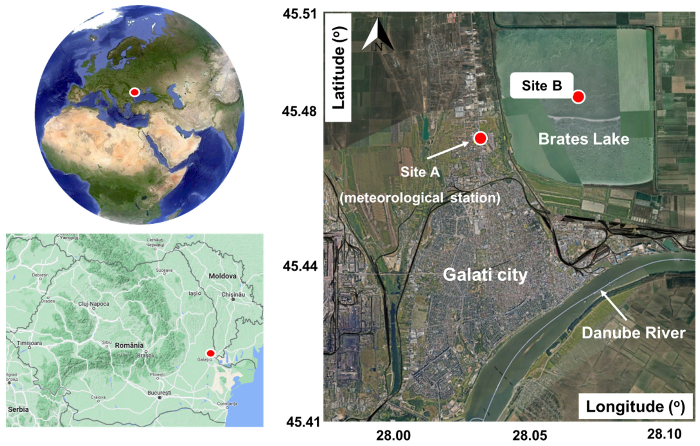
2.1. Study Area
2.2. Wind and Solar Datasets
2.3. Wind and Solar Systems
3. Results and Discussion
4. Conclusions
Author Contributions
Funding
Data Availability Statement
Acknowledgments
Conflicts of Interest
References
- Wang, J.; Mamkhezri, J.; Khezri, M.; Karimi, M.S.; Khan, Y.A. Insights from European Nations on the Spatial Impacts of Renewable Energy Sources on CO2 Emissions. Energy Rep. 2022, 8, 5620–5630. [Google Scholar] [CrossRef]
- Durakovic, G.; del Granado, P.C.; Tomasgard, A. Powering Europe with North Sea Offshore Wind: The Impact of Hydrogen Investments on Grid Infrastructure and Power Prices. Energy 2023, 263, 125654. [Google Scholar] [CrossRef]
- Wind Energy in Europe: 2022 Statistics and the Outlook for 2023–2027. Available online: https://windeurope.org/data-and-analysis/product/wind-energy-in-europe-2022-statistics-and-the-outlook-for-2023-2027 (accessed on 20 March 2023).
- Madsen, D.N.; Hansen, J.P. Outlook of Solar Energy in Europe Based on Economic Growth Characteristics. Renew. Sustain. Energy Rev. 2019, 114, 109306. [Google Scholar] [CrossRef]
- Kakoulaki, G.; Gonzalez Sanchez, R.; Gracia Amillo, A.; Szabo, S.; De Felice, M.; Farinosi, F.; De Felice, L.; Bisselink, B.; Seliger, R.; Kougias, I.; et al. Benefits of Pairing Floating Solar Photovoltaics with Hydropower Reservoirs in Europe. Renew. Sustain. Energy Rev. 2023, 171, 112989. [Google Scholar] [CrossRef]
- Agrawal, K.K.; Jha, S.K.; Mittal, R.K.; Vashishtha, S. Assessment of Floating Solar PV (FSPV) Potential and Water Conservation: Case Study on Rajghat Dam in Uttar Pradesh, India. Energy Sustain. Dev. 2022, 66, 287–295. [Google Scholar] [CrossRef]
- Mamatha, G.; Kulkarni, P.S. Assessment of Floating Solar Photovoltaic Potential in India’s Existing Hydropower Reservoirs. Energy Sustain. Dev. 2022, 69, 64–76. [Google Scholar] [CrossRef]
- Zuzana, D. Where Sun Meets Water: Floating Solar Handbook for Practitioners. Available online: https://documents.worldbank.org/pt/publication/documents-reports/documentdetail/418961572293438109/Where-Sun-Meets-Water-Floating-Solar-Handbook-for-Practitioners (accessed on 20 March 2023).
- Cebotari, S.; Cristea, M.; Moldovan, C.; Zubascu, F. Renewable Energy’s Impact on Rural Development in Northwestern Romania. Energy Sustain. Dev. 2017, 37, 110–123. [Google Scholar] [CrossRef]
- Ionescu, R.V.; Antohi, V.M.; Zlati, M.L.; Georgescu, L.P.; Iticescu, C. To a Green Economy across the European Union. Int. J. Environ. Res. Public Health 2022, 19, 12427. [Google Scholar] [CrossRef]
- Vrînceanu, A.; Dumitrașcu, M.; Kucsicsa, G. Site Suitability for Photovoltaic Farms and Current Investment in Romania. Renew. Energy 2022, 187, 320–330. [Google Scholar] [CrossRef]
- Onea, F.; Ciortan, S.; Rusu, E. Assessment of the Potential for Developing Combined Wind-Wave Projects in the European Nearshore. Energy Environ. 2017, 28, 580–597. [Google Scholar] [CrossRef]
- Dragomir, G.; Șerban, A.; Năstase, G.; Brezeanu, A.I. Wind Energy in Romania: A Review from 2009 to 2016. Renew. Sustain. Energy Rev. 2016, 64, 129–143. [Google Scholar] [CrossRef]
- Onea, F.; Rusu, L. A Study on the Wind Energy Potential in the Romanian Coastal Environment. J. Mar. Sci. Eng. 2019, 7, 142. [Google Scholar] [CrossRef]
- Răileanu, A.B.; Rusu, L.; Rusu, E. An Evaluation of the Dynamics of Some Meteorological and Hydrological Processes along the Lower Danube. Sustainability 2023, 15, 6087. [Google Scholar] [CrossRef]
- Business Romania. Latest News from Business in Romania Only at ZF English. Available online: https://www.zfenglish.com/ (accessed on 21 March 2023).
- LIBERTY Galati GREENSTEEL Transformation Plan. Available online: https://libertysteelgroup.com/delivering_cn30/liberty-galati-greensteel-transformation-plan/ (accessed on 22 March 2023).
- Constantin, D.-E.; Bocăneala, C.; Voiculescu, M.; Roşu, A.; Merlaud, A.; Roozendael, M.V.; Georgescu, P.L. Evolution of SO2 and NOx Emissions from Several Large Combustion Plants in Europe during 2005–2015. Int. J. Environ. Res. Public Health 2020, 17, 3630. [Google Scholar] [CrossRef] [PubMed]
- Popa, P.; Murariu, G.; Timofti, M.; Georgescu, L.P. Multivariate Statistical Analyses of Danube River Water Quality at Galati, Romania. Environ. Eng. Manag. J. 2018, 17, 1249–1266. [Google Scholar] [CrossRef]
- Ţuţuianu, L.; Vespremeanu-Stroe, A.; Preoteasa, L.; Rotaru, S.; Dima, A.; Dimofte, D. Wetlands and Lakes Formation and Evolution on the Lower Danube Floodplain during Middle and Late Holocene. Quat. Int. 2021, 602, 82–91. [Google Scholar] [CrossRef]
- Avram, S.; Cipu, C.; Corpade, A.-M.; Gheorghe, C.A.; Manta, N.; Niculae, M.-I.; Pascu, I.S.; Szép, R.E.; Rodino, S. GIS-Based Multi-Criteria Analysis Method for Assessment of Lake Ecosystems Degradation—Case Study in Romania. Int. J. Environ. Res. Public Health 2021, 18, 5915. [Google Scholar] [CrossRef]
- Banescu, A.; Arseni, M.; Georgescu, L.P.; Rusu, E.; Iticescu, C. Evaluation of Different Simulation Methods for Analyzing Flood Scenarios in the Danube Delta. Appl. Sci. 2020, 10, 8327. [Google Scholar] [CrossRef]
- Ion, I.M.D.; Dincă, C.S.; Șerban, C.B.; Stanciu, S. Agricultural Sector in Galaţi County. Resources for the Seed Production. In Proceedings of the 31st International Business Information Management Association Conference, Milan, Italy, 25–26 April 2018; International Business Information Management Association (IBIMA): King of Prussia, PA, USA, 2018. [Google Scholar]
- Calmuc, M.; Calmuc, V.; Arseni, M.; Topa, C.; Timofti, M.; Georgescu, L.P.; Iticescu, C. A Comparative Approach to a Series of Physico-Chemical Quality Indices Used in Assessing Water Quality in the Lower Danube. Water 2020, 12, 3239. [Google Scholar] [CrossRef]
- Apetrei, C.; Iticescu, C.; Georgescu, L.P. Multisensory System Used for the Analysis of the Water in the Lower Area of River Danube. Nanomaterials 2019, 9, 891. [Google Scholar] [CrossRef]
- Calmuc, V.A.; Calmuc, M.; Arseni, M.; Topa, C.M.; Timofti, M.; Burada, A.; Iticescu, C.; Georgescu, L.P. Assessment of Heavy Metal Pollution Levels in Sediments and of Ecological Risk by Quality Indices, Applying a Case Study: The Lower Danube River, Romania. Water 2021, 13, 1801. [Google Scholar] [CrossRef]
- Guillory, A. ERA5. Available online: https://www.ecmwf.int/en/forecasts/datasets/reanalysis-datasets/era5 (accessed on 31 May 2019).
- Soukissian, T.H.; Karathanasi, F.E.; Zaragkas, D.K. Exploiting Offshore Wind and Solar Resources in the Mediterranean Using ERA5 Reanalysis Data. Energy Convers. Manag. 2021, 237, 114092. [Google Scholar] [CrossRef]
- Jurasz, J.; Mikulik, J.; Dąbek, P.B.; Guezgouz, M.; Kaźmierczak, B. Complementarity and ‘Resource Droughts’ of Solar and Wind Energy in Poland: An ERA5-Based Analysis. Energies 2021, 14, 1118. [Google Scholar] [CrossRef]
- Bouallègue, Z.B.; Cooper, F.; Chantry, M.; Düben, P.; Bechtold, P.; Sandu, I. Statistical Modeling of 2-m Temperature and 10-m Wind Speed Forecast Errors. Mon. Weather. Rev. 2023, 151, 897–911. [Google Scholar] [CrossRef]
- Archer, C.L.; Jacobson, M.Z. Evaluation of Global Wind Power. J. Geophys. Res. Atmos. 2005, 110, 1–20. [Google Scholar] [CrossRef]
- Liu, B.; Ma, X.; Guo, J.; Li, H.; Jin, S.; Ma, Y.; Gong, W. Estimating Hub-Height Wind Speed Based on a Machine Learning Algorithm: Implications for Wind Energy Assessment. Atmos. Chem. Phys. 2023, 23, 3181–3193. [Google Scholar] [CrossRef]
- de Souza Nascimento, M.M.; Shadman, M.; Silva, C.; de Freitas Assad, L.P.; Estefen, S.F.; Landau, L. Offshore Wind and Solar Complementarity in Brazil: A Theoretical and Technical Potential Assessment. Energy Convers. Manag. 2022, 270, 116194. [Google Scholar] [CrossRef]
- Khalifeh Soltani, S.R.; Mostafaeipour, A.; Almutairi, K.; Hosseini Dehshiri, S.J.; Hosseini Dehshiri, S.S.; Techato, K. Predicting Effect of Floating Photovoltaic Power Plant on Water Loss through Surface Evaporation for Wastewater Pond Using Artificial Intelligence: A Case Study. Sustain. Energy Technol. Assess. 2022, 50, 101849. [Google Scholar] [CrossRef]
- Hayibo, K.S.; Pearce, J.M. Foam-Based Floatovoltaics: A Potential Solution to Disappearing Terminal Natural Lakes. Renew. Energy 2022, 188, 859–872. [Google Scholar] [CrossRef]
- Mittal, D.; Kumar Saxena, B.; Rao, K.V.S. Potential of Floating Photovoltaic System for Energy Generation and Reduction of Water Evaporation at Four Different Lakes in Rajasthan. In Proceedings of the 2017 International Conference on Smart Technologies For Smart Nation (SmartTechCon), Bengaluru, India, 17–19 August 2017; IEEE: Piscataway, NJ, USA, 2017; pp. 238–243. [Google Scholar]
- Urraca, R.; Gracia-Amillo, A.M.; Koubli, E.; Huld, T.; Trentmann, J.; Riihelä, A.; Lindfors, A.V.; Palmer, D.; Gottschalg, R.; Antonanzas-Torres, F. Extensive Validation of CM SAF Surface Radiation Products over Europe. Remote Sens. Environ. 2017, 199, 171–186. [Google Scholar] [CrossRef]
- Riihelä, A.; Kallio, V.; Devraj, S.; Sharma, A.; Lindfors, A.V. Validation of the SARAH-E Satellite-Based Surface Solar Radiation Estimates over India. Remote Sens. 2018, 10, 392. [Google Scholar] [CrossRef]
- V162-6.2 MWTM. Available online: https://www.vestas.com/en/products/enventus-platform/v162-6-2-mw (accessed on 16 May 2023).
- Welcome to Wind-Turbine-Models.Com. Available online: https://en.wind-turbine-models.com/ (accessed on 20 May 2018).
- Wind Energy Database. Available online: https://www.thewindpower.net/index.php (accessed on 1 May 2019).
- Rusu, E. An Evaluation of the Wind Energy Dynamics in the Baltic Sea, Past and Future Projections. Renew. Energy 2020, 160, 350–362. [Google Scholar] [CrossRef]
- Rusu, E.; Onea, F. A Parallel Evaluation of the Wind and Wave Energy Resources along the Latin American and European Coastal Environments. Renew. Energy 2019, 143, 1594–1607. [Google Scholar] [CrossRef]
- López, M.; Rodríguez, N.; Iglesias, G. Combined Floating Offshore Wind and Solar PV. J. Mar. Sci. Eng. 2020, 8, 576. [Google Scholar] [CrossRef]
- López, M.; Soto, F.; Hernández, Z.A. Assessment of the Potential of Floating Solar Photovoltaic Panels in Bodies of Water in Mainland Spain. J. Clean. Prod. 2022, 340, 130752. [Google Scholar] [CrossRef]
- Manolache, A.I.; Andrei, G.; Rusu, L. An Evaluation of the Efficiency of the Floating Solar Panels in the Western Black Sea and the Razim-Sinoe Lagunar System. J. Mar. Sci. Eng. 2023, 11, 203. [Google Scholar] [CrossRef]
- Maraj, A.; Kërtusha, X.; Lushnjari, A. Energy Performance Evaluation for a Floating Photovoltaic System Located on the Reservoir of a Hydro Power Plant under the Mediterranean Climate Conditions during a Sunny Day and a Cloudy-One. Energy Convers. Manag. X 2022, 16, 100275. [Google Scholar] [CrossRef]
- Fereshtehpour, M.; Javidi Sabbaghian, R.; Farrokhi, A.; Jovein, E.B.; Ebrahimi Sarindizaj, E. Evaluation of Factors Governing the Use of Floating Solar System: A Study on Iran’s Important Water Infrastructures. Renew. Energy 2021, 171, 1171–1187. [Google Scholar] [CrossRef]
- Hersbach, H.; Bell, B.; Berrisford, P.; Hirahara, S.; Horányi, A.; Muñoz-Sabater, J.; Nicolas, J.; Peubey, C.; Radu, R.; Schepers, D.; et al. The ERA5 Global Reanalysis. Q. J. R. Meteorol. Soc. 2020, 146, 1999–2049. [Google Scholar] [CrossRef]
- Wang, H.; Blaabjerg, F.; Ma, K.; Wu, R. Design for Reliability in Power Electronics in Renewable Energy Systems–Status and Future. In Proceedings of the 4th International Conference on Power Engineering, Energy and Electrical Drives, Istanbul, Turkey, 13–17 May 2013; IEEE: Piscataway, NJ, USA, 2013; pp. 1846–1851. [Google Scholar]
- Abed, K.A.; El-Mallah, A.A. Capacity Factor of Wind Turbines. Energy 1997, 22, 487–491. [Google Scholar] [CrossRef]
- Michalco, B.T. Kim Tranberg and David Statistics. Available online: https://turbines.dk/statistics (accessed on 3 April 2023).
- Staffell, I.; Green, R. How Does Wind Farm Performance Decline with Age? Renew. Energy 2014, 66, 775–786. [Google Scholar] [CrossRef]
- Boretti, A.; Castelletto, S. Trends in Performance Factors of Wind Energy Facilities. SN Appl. Sci. 2020, 2, 1718. [Google Scholar] [CrossRef]
- Gonzalez Sanchez, R.; Kougias, I.; Moner-Girona, M.; Fahl, F.; Jäger-Waldau, A. Assessment of Floating Solar Photovoltaics Potential in Existing Hydropower Reservoirs in Africa. Renew. Energy 2021, 169, 687–699. [Google Scholar] [CrossRef]
- Padilha Campos Lopes, M.; Nogueira, T.; Santos, A.J.L.; Castelo Branco, D.; Pouran, H. Technical Potential of Floating Photovoltaic Systems on Artificial Water Bodies in Brazil. Renewable Energy 2022, 181, 1023–1033. [Google Scholar] [CrossRef]
- Resources.Solarbusinesshub.com. Floating Solar Photovoltaic (FSPV): A Third Pillar to Solar PV Sector? Available online: https://resources.solarbusinesshub.com/solar-industry-reports/item/floating-solar-photovoltaic-fspv-a-third-pillar-to-solar-pv-sector (accessed on 4 April 2023).
- Pouran, H.; Padilha Campos Lopes, M.; Ziar, H.; Alves Castelo Branco, D.; Sheng, Y. Evaluating Floating Photovoltaics (FPVs) Potential in Providing Clean Energy and Supporting Agricultural Growth in Vietnam. Renew. Sustain. Energy Rev. 2022, 169, 112925. [Google Scholar] [CrossRef]
- Wang, Z.; Nguyen, T.; Westerhoff, P. Food–Energy–Water Analysis at Spatial Scales for Districts in the Yangtze River Basin (China). Environ. Eng. Sci. 2019, 36, 789–797. [Google Scholar] [CrossRef]
- Bao, Q.; Ding, J.; Han, L.; Li, J.; Ge, X. Predicting Land Change Trends and Water Consumption in Typical Arid Regions Using Multi-Models and Multiple Perspectives. Ecol. Indic. 2022, 141, 109110. [Google Scholar] [CrossRef]
- Vezzoni, R. Green Growth for Whom, How and Why? The REPowerEU Plan and the Inconsistencies of European Union Energy Policy. Energy Res. Soc. Sci. 2023, 101, 103134. [Google Scholar] [CrossRef]


| Location | ID | Data Type | Parameter | Latitude (°) | Longitude (°) |
|---|---|---|---|---|---|
| Galati | Site A | In situ, ERA5 | U10 | 45.473 | 28.032 |
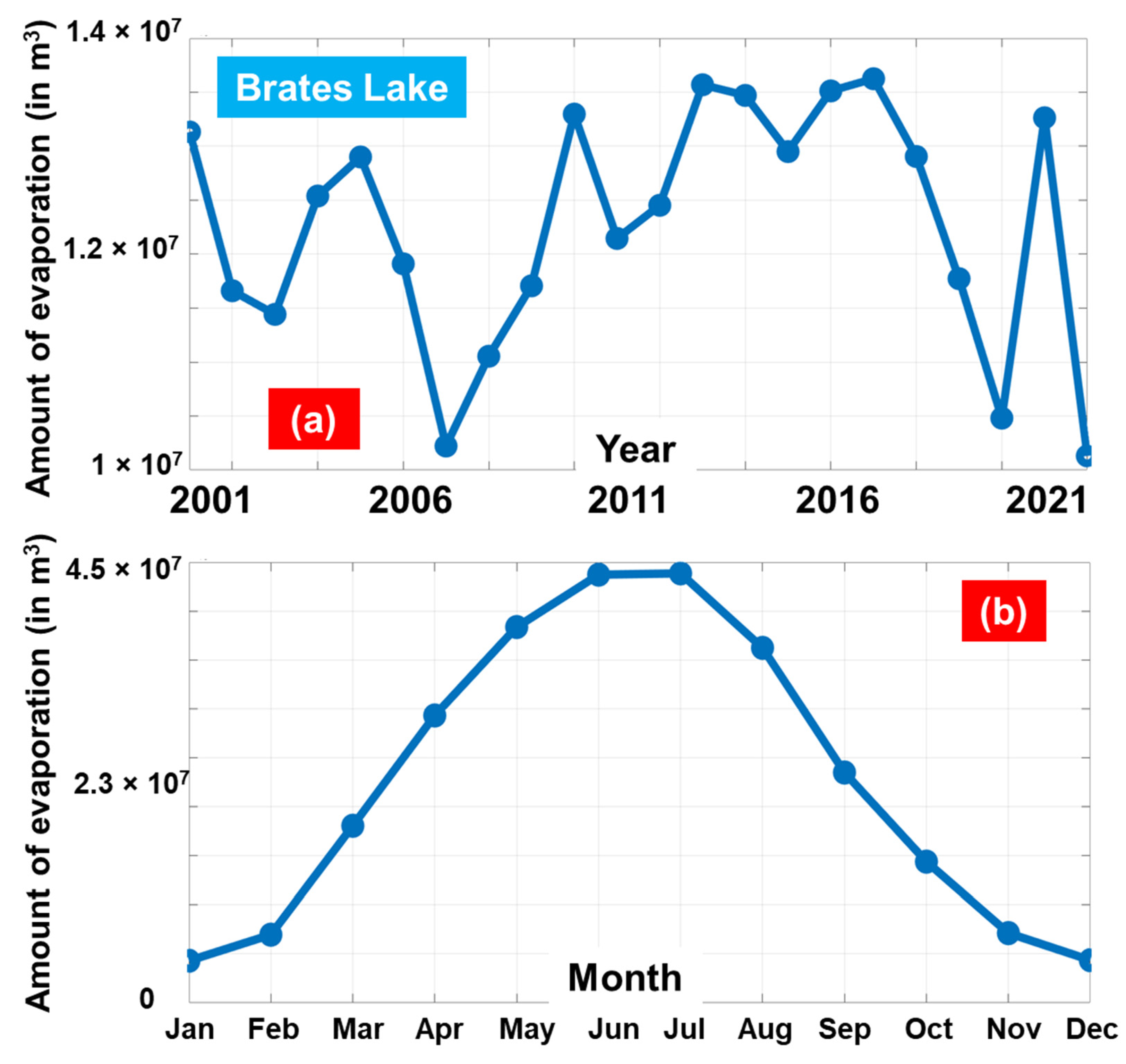
| Galati | Site B | ERA5, SARAH | U100, SSRD, Temp, Evaporation | 45.483 | 28.070 |
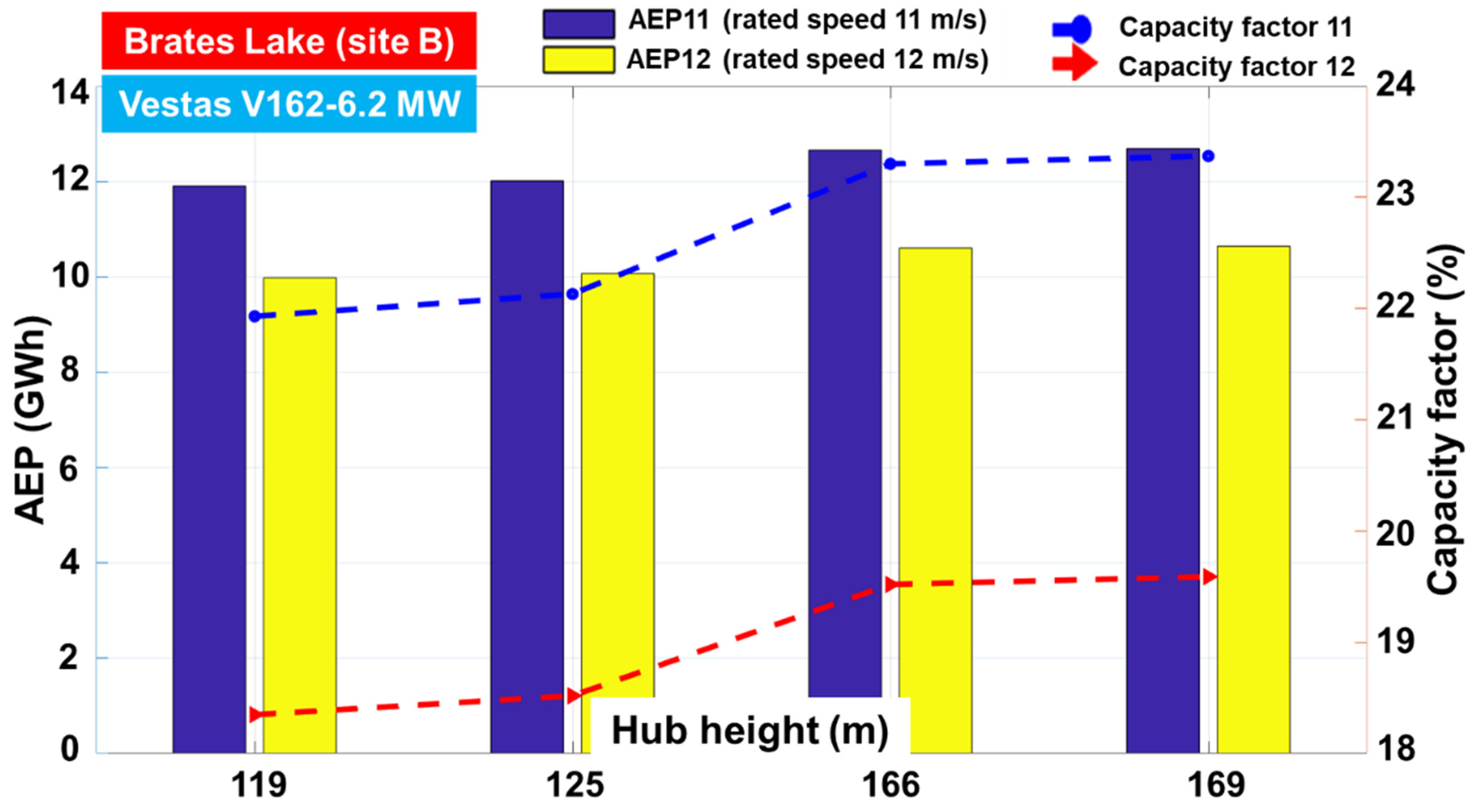
| Turbine | Rated Power (MW) | Cut-In Speed (m/s) | Rated Speed (m/s) | Cut-Out Speed (m/s) | Hub Height (m) |
|---|---|---|---|---|---|
| General Electric 2.5xl (T1) | 2.5 | 3.5 | 13.5 | 25 | 75/100 |
| Vestas V90-2.0 (T2) | 2 | 4 | 13 | 25 | 80/95/105 |
| Enercon E82-E2 (T3) | 2 | 2 | 12.5 | 25 | 78/85/98/108/138 |
| Gamesa G90 (T4) | 2 | 3 | 11 | 21 | 67/78/90/100 |
| Vestas V162-6.2 MW | 6.2 | 3 | N/A | 25 | 119/125/166/169 |
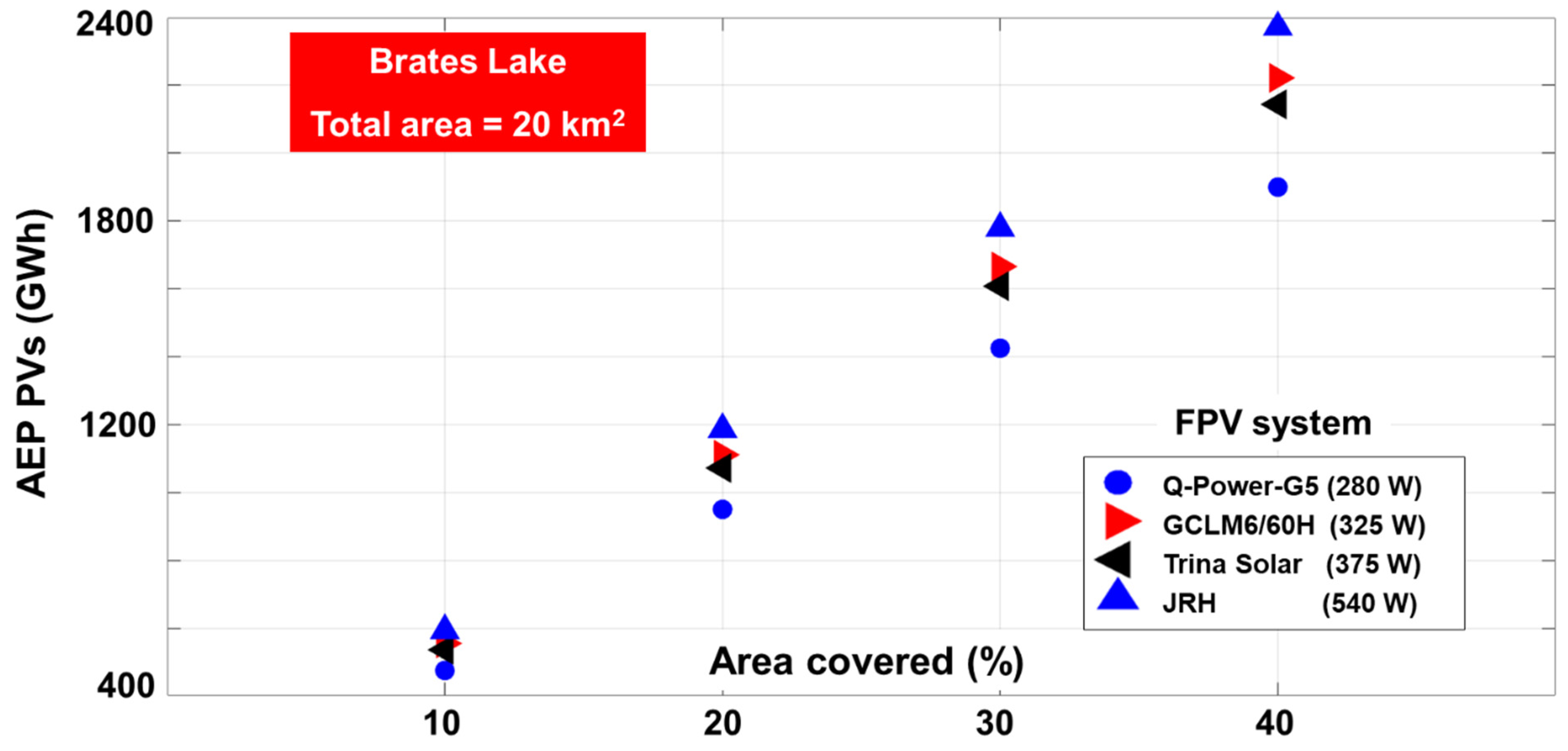
| Parameter | Q-Power-G5 280 (P1) | GCLM6/60H-325 (P2) | Trina Solar (P3) | JRH 540 W (P4) |
|---|---|---|---|---|
| Power (W) | 280 | 325 | 375 | 540 |
| Efficiency (%) | 17.10 | 20.00 | 19.30 | 21.35 |
| Surface (m2) | 1.94 | 1.62 | 1.95 | 2.58 |
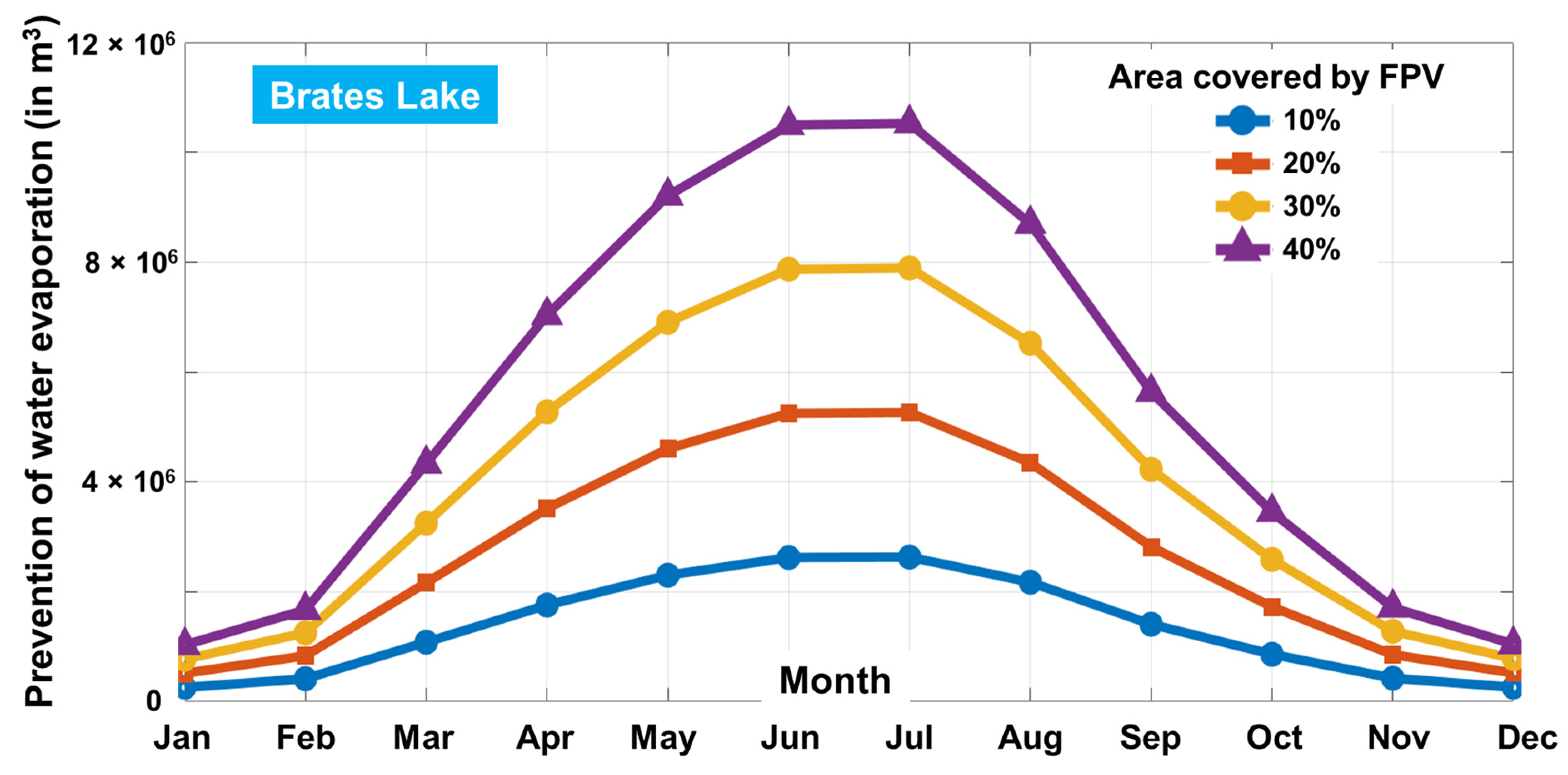
| FPV System | Brates Lake—Scenarios | |||
|---|---|---|---|---|
| 10% (2 km2) | 20% (4 km2) | 30% (6 km2) | 40% (8 km2) | |
| Q-Power-G5 280 | 289 | 577 | 866 | 1155 |
| GCLM6/60H-325 | 401 | 802 | 1204 | 1605 |
| Trina Solar | 385 | 769 | 1154 | 1538 |
| JRH 540 W | 418 | 836 | 1254 | 1672 |
| Turbine | Hub Height (m) | |||||||||||
|---|---|---|---|---|---|---|---|---|---|---|---|---|
| 67 | 75 | 78 | 80 | 85 | 90 | 95 | 98 | 100 | 105 | 108 | 138 | |
| T1 | 11.91 | 12.68 | ||||||||||
| T2 | 11.71 | 12.2 | 12.49 | |||||||||
| T3 | 17.82 | 18.08 | 18.53 | 18.83 | 19.61 | |||||||
| T4 | 19.64 | 20.24 | 20.81 | 21.23 | ||||||||
Disclaimer/Publisher’s Note: The statements, opinions and data contained in all publications are solely those of the individual author(s) and contributor(s) and not of MDPI and/or the editor(s). MDPI and/or the editor(s) disclaim responsibility for any injury to people or property resulting from any ideas, methods, instructions or products referred to in the content. |
© 2023 by the authors. Licensee MDPI, Basel, Switzerland. This article is an open access article distributed under the terms and conditions of the Creative Commons Attribution (CC BY) license (https://creativecommons.org/licenses/by/4.0/).
Share and Cite
Rusu, E.; Georgescu, P.L.; Onea, F.; Yildirir, V.; Dragan, S. The Potential of Lakes for Extracting Renewable Energy—A Case Study of Brates Lake in the South-East of Europe. Inventions 2023, 8, 143. https://doi.org/10.3390/inventions8060143
Rusu E, Georgescu PL, Onea F, Yildirir V, Dragan S. The Potential of Lakes for Extracting Renewable Energy—A Case Study of Brates Lake in the South-East of Europe. Inventions. 2023; 8(6):143. https://doi.org/10.3390/inventions8060143
Chicago/Turabian StyleRusu, Eugen, Puiu Lucian Georgescu, Florin Onea, Victoria Yildirir, and Silvia Dragan. 2023. "The Potential of Lakes for Extracting Renewable Energy—A Case Study of Brates Lake in the South-East of Europe" Inventions 8, no. 6: 143. https://doi.org/10.3390/inventions8060143
APA StyleRusu, E., Georgescu, P. L., Onea, F., Yildirir, V., & Dragan, S. (2023). The Potential of Lakes for Extracting Renewable Energy—A Case Study of Brates Lake in the South-East of Europe. Inventions, 8(6), 143. https://doi.org/10.3390/inventions8060143