Abstract
Plastic pervasiveness in daily life has increased in tandem with population growth. Ethylene–vinyl acetate (EVA) is emerging as a popular compound for manufacturing plastic, which is obtained from ethylene and vinyl acetate synthesis. EVA is produced using autoclave reactors, which often encounter bearing damage under specific operating conditions. This research aims to optimize the parameters in autoclave reactors to enhance bearing life. The study focuses on two crucial factors: the number of impellers and the temperature, with bearing life as the response variable. Simulations using finite-element analysis were conducted to obtain the fatigue life of bearings and validated using real-time company data stating the damage of bearings within 80 days. The optimization process employed the Taguchi method (TM) and the response surface methodology (RSM). A comparison of these techniques revealed that temperature had the most significant influence on the response. Interestingly, both methods yielded the same optimal parameters: seven impellers and a temperature of 150 °C. The simulation results using these optimized parameters demonstrated a noteworthy 3.095% increase in bearing life compared to the initial design. The RSM outperformed the Taguchi method in accurately predicting response values with minimum prediction error under optimal conditions.
1. Introduction
Plastic production has become a significant focus for many countries due to the high demand for plastic products. Ethylene–vinyl acetate (EVA) is a popular type of plastic widely used in various applications. The primary method employed for EVA production is high-pressure continuous bulk polymerization, which includes autoclave and tubular processes. Among these, the autoclave process is particularly interesting due to its higher percentage of vinyl acetate content, enhancing EVA applications’ versatility. EVA production in the autoclave process using an autoclave reactor has several problems that can occur in autoclave reactors, such as leaks in valves, overpressure, explosions due to excessive exothermic reactions, bearing damage, and others [1,2,3,4,5,6,7,8,9]. One of the critical problems that occurs in autoclave reactors is bearing damage. Changes in impeller design and working conditions will be analyzed to maximize bearing life.
Several studies have focused on optimizing ethylene–vinyl acetate (EVA) production in autoclave reactors. Lee et al. [6] used computational fluid dynamics (CFD) to analyze the stirrer’s mixing effect in a multicompartment model of an autoclave reactor with operating temperatures ranging from 150 to 300 °C and pressures ranging from 130 to 300 MPa. The model predicted the local temperature and properties of the polymer product by simulating hydrodynamics and polymerization kinetics. However, the model had limitations, such as failing to account for micro-admixture in the reactor and short-chain branching caused by the backbiting mechanism. Brandolin et al. [10] proposed a mathematical model for the molecular weight distribution of polyethylene and ethylene–vinyl acetate copolymers in an autoclave reactor. Their method used transformed mass balance equations and probability-generating function transformations to predict economic benefits and molecular safety. Wang et al. [11] investigated the effect of impeller speed on fluid flow and temperature distribution in an autoclave reactor using computational fluid dynamics (CFD). Increasing the speed of the impeller improved fluid mixing, temperature homogeneity, and initiator efficiency. Torotwa and Changying [12] used CFD to investigate the effect of different impeller shapes on flow characteristics in mixing systems. Counter-flow and saw-tooth impellers produced uniform flows, whereas anchor and Rushton impellers focused flow in specific areas, producing higher product quality. Furthermore, studies in the literature [1,2,3,4,5,6,7,8] have discussed common problems in autoclave reactors, such as bearing damage, abnormal pressures and temperatures, and leaks. A critical problem in autoclave reactors is damage to the bearings. Since damage to the bearings will disrupt the production of ethylene–vinyl acetate (EVA), because the reactor must be shut down during repairs, several benefits can be obtained by maximizing the life of the bearings, including reducing the time wasted, because the autoclave reactor must be turned off during the maintenance process; increasing the operating time of the autoclave reactor; increasing total production (due to increased operating time and reduced maintenance time); and reducing costs for the maintenance process and purchase of spare parts. It can be said that maximizing the bearing life can decrease the overall production cost. Figure 1 depicts a visualization of bearing damage in an autoclave reactor. Thus, increasing bearing life reduces downtime, improves production efficiency, and lowers maintenance costs. Chien et al. [13] explained the relationship between increasing autoclave working temperature and production yield. In comparison, Pladis et al. [14] optimized the performance of mixing ethylene and vinyl acetate in an autoclave reactor operating at a temperature of 220–260 °C.
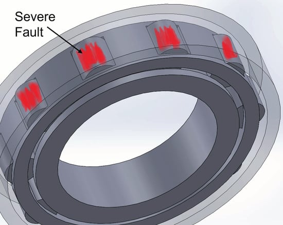
Figure 1.
Visualization of damage in failed bearings. Reprinted/adapted with permission from refs. [5,9].
In the realm of chemical engineering, the Taguchi method (TM) [15] and the response surface methodology (RSM) [16] stand as indispensable optimization tools. Zhou et al. employed the TM to optimize thiocarbohydrazide (TCH) synthesis, emphasizing key factors like reflux time and temperature, achieving a remarkable 92.3% yield [17]. Meanwhile, Bello et al. [18] used a central composite design and the response surface methodology to optimize biodiesel production, reaching a 91.6% yield and demonstrating the critical impact of parameters such as reaction time and temperature. Furthermore, Said et al.’s [19] work emphasizes the RSM’s significance in optimizing extraction processes for food plants and herbs, effectively demonstrating the efficiency of techniques such as central composite design and the Box–Behnken approach. Liang et al. demonstrated a novel computational fluid dynamics (CFD) and RSM-based method that optimizes fibrous filtration design by accounting for the synergetic effects of filtration parameters, enhancing efficiency [20]. Lu et al. [21] developed an efficient reliability calculation method that integrates response surface methodology (RSM) and the advanced first-order second-moment method (AFOSM) under elastohydrodynamic lubrication (EHL) conditions for specialized rolling bearings. an efficient reliability calculation method for specialized rolling bearings. It reduces time consumption compared to traditional methods while maintaining high accuracy in contact fatigue reliability analysis. The extensive fatigue testing required for bearings presents substantial challenges, rendering conventional methods impractical. The RSM and Taguchi-based optimization methods provide advanced computational solutions, allowing for precise prediction and optimization of bearing life without the necessity for extensive physical testing. This integration yields a profound understanding of the intricate factors impacting bearing performance. These optimization methodologies have greatly revolutionized the field of chemical engineering by streamlining experiments, preserving resources, and attaining optimal results with heightened precision and efficiency.
This research aimed to enhance bearing life in an autoclave reactor by analyzing changes in impeller design and working conditions. The study employed an FEA using Ansys 2022 R2 software and optimized the process using the Taguchi method™ and the response surface methodology (RSM). The independent variables or factors considered included the number of impellers and temperature. Data were analyzed using methods such as ANOVA, S/N ratios, response contours, and Pareto graphs of common effects with the assistance of Minitab 21 software. The research aimed to determine the effects of the number of impellers and temperature based on simulations, compare the results obtained via the Taguchi method and the RSM, and identify the optimal parameters for the number of impellers and temperature to maximize bearing life.
2. Theoretical Background
2.1. Ethylene–Vinyl Acetate (EVA)
Ethylene–vinyl acetate (EVA) is a thermoplastic resin synthesized by combining ethylene and vinyl acetate, as shown in Figure 2. It was first developed in the 1930s and has since been widely used [22]. The copolymerization process offers adjustable vinyl acetate ratios to modify polymer properties. Continuous or batch processes influence EVA’s melting point based on vinyl acetate content. EVA is highly flexible, impact-resistant, and tough in low temperatures, making it ideal for cold and flexible applications. It possesses low density, good electrical insulation, weather resistance, adhesion, chemical resistance, and low toxicity, enabling its versatility across multiple applications. EVA is versatile in its applications, including adhesives in tapes, labels, and packaging; coatings for wires, flooring, and auto parts; hot-melt sealants in shoes and toys; cushioning in footwear and sports gear; food packaging materials; flexible packaging and molded products; lightweight toys; medical devices; and insulation in electrical and thermal applications.
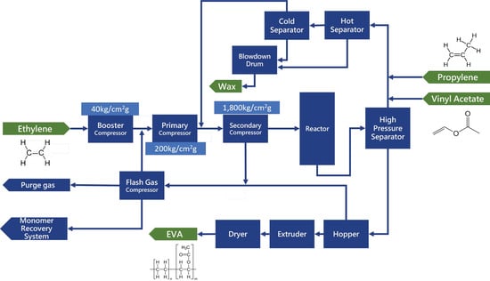
Figure 2.
EVA synthesis. Reprinted/adapted with permission from ref. [23].
2.2. EVA Autoclave Reactor Systems
An autoclave reactor is a long, tubular vessel divided into different zones designed for high-pressure, high-temperature reactions, as shown in Figure 3. Operating as a continuous stirred tank reactor (CSTR), it provides efficient mixing of chemicals. Primarily used for small-scale production, autoclave reactors offer a conversion rate of around 22% for ethylene–vinyl acetate (EVA) synthesis. Autoclave reactors produce approximately 100,000 tons of EVA per year. They also enable the production of EVA with a higher vinyl acetate (VA) content, exceeding 40% and operating at temperatures of 150–300 °C and pressures of 100–300 MPa. Autoclave reactors utilize impellers or blades for effective fluid mixing, which play a crucial role in the reactors’ performance. Overall, autoclave reactors serve as specialized vessels for high-pressure, high-temperature reactions and are particularly suitable for small-scale EVA production with higher VA content.

Figure 3.
Autoclave reactor. Reprinted/adapted with permission from ref. [5].
2.3. Blade Types in EVA Autoclave Reactors
Fluid mixing, a crucial process in an autoclave reactor, is significantly affected by the blade’s shape. The blade’s design plays a pivotal role in the mixing efficiency because it forms part of the impeller and the hub. The hub, directly connected to the shaft, is coupled to the blade through welding or screws. Welding is preferred for hub-blade attachment, as it minimizes material buildup on bolts and fittings. Current studies delve into various autoclave blade types and their associated flow characteristics, recognizing their significant influence on the homogenization process and the resultant flow patterns. Flow patterns are categorized into three types: axial flow, radial flow, and tangential flow. Axial-flow impellers, exemplified by hydrofoil blades, generate parallel flow along the axis of rotation, effectively preventing settling at the tank’s bottom, and are well-suited for low- to medium-viscosity fluids. Radial-flow impellers, as seen in paddle blades and Rushton blades, create perpendicular flow relative to the axis of rotation, enabling the mixing of gas–liquid and liquid–liquid mixtures. Tangential-flow impellers, typified by anchor blades, induce circular flow around the shaft, making them ideal for blending highly viscous media. A profound comprehension of these diverse blade shapes and their corresponding flow patterns is pivotal for enhancing mixing performance within autoclave reactors, ultimately contributing to process efficiency and product quality.
2.4. Bearing Types in EVA Autoclave Reactors
Bearings are essential components that reduce the load resulting from rotation. They come in two main types: sliding bearings (like journal and linear bearings) and rolling bearings (including ball and roller bearings). Rolling bearings are widely used in various pieces of machinery thanks to their efficiency in reducing friction through rolling instead of sliding. This characteristic, combined with reduced lubrication requirements and the ability to withstand high speeds and heavy loads, justifies their designation as “anti-friction bearings”. Bearings consist of four main parts: an outer ring, an inner ring, rolling elements (balls or rollers), and a separator (cage). These components work together, as one ring may rotate while the other remains still, with rolling elements riding between them. A cage keeps the elements evenly spaced to minimize friction. Seals or dust shields can be added for protection against contaminants. Ball bearings (NSK 7322B) and roller bearings (NSK 224 M/FAG 224) are used in autoclave reactors.
Ball bearings excel at high rotational speeds with moderate radial and axial loads due to their brief contact with the races, enabling smooth rotation. Conversely, roller bearings are preferred for heavier radial and lighter axial loads thanks to their larger contact surface area that resists deformation under heavy loads. Bearing failures may result from a variety of factors, including imbalance, misalignment, loose rotation axes, debris contamination, inadequate lubrication, deformation, fatigue, and wear. These issues are often associated with operator error, environmental conditions, and challenging working environments, thereby ensuring that the meaning is preserved. Bearings, operating at high speeds and significant loads, are susceptible to failure, making it essential to assess their durability through life-cycle calculations [24].
Bearing life is the expected duration of a bearing function under specific conditions, often measured by the number of revolutions before signs of fatigue appear. L10, indicating 1 million revolutions, is a standard metric. Designers consider the application’s operational needs to determine actual service life. A life-cycle calculation is performed to assess the bearing’s durability, considering factors like the dynamic load rating and temperature adjustment. Bearing life is estimated based on the number of revolutions before signs of fatigue appear. The mathematical model of bearing-life rating can be seen in Equation (1).
where is the dynamic equivalent bearing load (), is the dynamic load rating (), and is the exponent (3 for ball bearings, 10/3 for roller bearings).
The dynamic equivalent load () and the temperature factor play a role in determining a bearing’s rated service life. Bearing steel loses hardness if bearings are used at high operating temperatures. The nominal speed should, therefore, be adjusted for higher temperatures using Equation (2):
where is the basic load rating before temperature adjustment () and is the temperature factor.
3. Methodology
The methodology for conducting the research is outlined with a flowchart of the steps involved (Figure 4). The process initiated with the commencement of research, followed by a comprehensive literature review. Subsequently, the selection of variables (factors) and the creation of an experimental design were performed. Ansys 2022 R2 software was then utilized for conducting simulations to obtain bearing-life data. The acquired data from Ansys were subjected to validation against company data. If the validation error value fell below 10%, the process advanced; otherwise, a new experimental design was employed to improve the results. The subsequent stages involved model creation and optimization, employing the Taguchi method and the RSM. Following optimization, the results were assessed for acceptability. If the outcome was deemed unacceptable, the variable selection was revisited. However, if the result was satisfactory, the optimal variable was determined, culminating in the completion of the research.
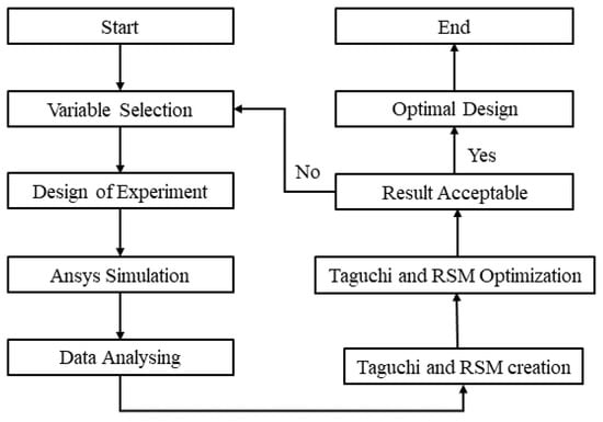
Figure 4.
Methodology flowchart.
3.1. Geometry of an Autoclave Reactor
This study used an autoclave reactor to perform EVA synthesis, whose specification was obtained from the EVA production company. There are three main components in an autoclave reactor, namely, an autoclave tank, a shaft and impeller, and bearings. Details about the locations of the components in the autoclave reactor can be seen in Figure 5.
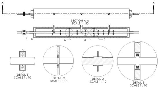
Figure 5.
Components of autoclave reactor. (A) Shaft. (B) Top bearing. (C) Mid bearing. (D) Impeller. (E) Bottom bearing.
The autoclave reactor featured a cylindrical tank with a height of 6.7 m, a diameter of 0.75 m, and a thickness of 15 cm, offering a total capacity of around 1800 L, with a length-to-diameter ratio of approximately 9:1. This design choice aligned with previous studies that favored cylindrical shapes for simulation-based research to simplify the geometry and reduce computational complexity [25]. The impeller shaft, spanning 8.9 m, incorporated nine turbine blade-type impellers pitched at 10 degrees for optimal energy efficiency. These impellers adhered to the 1/3 tank diameter rule. Three bearings were utilized: an NSK 7322B at the top, an NSK 224M as a mid bearing, and an FAG 224 at the bottom. NSK bearings have dimensions of a 110 mm inner diameter, a 240 mm outer diameter, and a 50 mm height, all of which are indicative of ball bearings. Conversely, NSK 224M and FAG 224 bearings are roller bearings featuring a 120 mm inner diameter, a 215 mm outer diameter, and a 40 mm height. Detailed technical drawings of individual components of the autoclave reactor are presented in Figure 6.
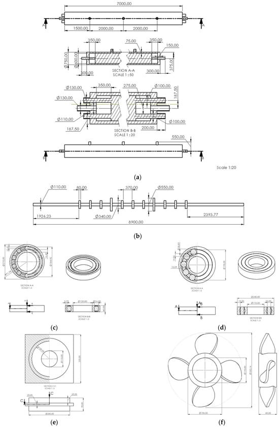
Figure 6.
Technical drawings of the autoclave reactor. (a) Tank assembly. (b) Shaft arrangement. (c) NSK 224 bearing. (d) NSK 7322B bearing. (e) Bearing housing. (f) Impeller blade.
Figure 7a illustrates the overall design of the autoclave reactor used for the simulations. Figure 7b shows the CAD design of the mid bearing (left) and the bottom bearing (right), while Figure 7c illustrates the impeller design with pitched turbine blades having a diameter 1/3 the diameter of the tank [26,27]. Table 1 provides a summary of the specifications of the tank, shaft, and bearing sizes of the autoclave reactor used in this study.
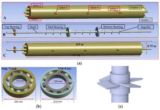
Figure 7.
CAD design of the autoclave reactor components used for simulations. (a) Complete design (A—outer casing of the reactor, B—inner shaft with bearing and impeller, C—total assembly). (b) Mid-bearing design. (c) Impeller design.

Table 1.
Specifications of autoclave reactor used in this study.
3.2. Design of the Experiment for the Taguchi Method and the Response Surface Methodology
In this research, the Taguchi method (TM) and the response surface methodology (RSM) were utilized as optimization techniques, employing different Design of Experiments (DOE) approaches. The TM employed an orthogonal array for the DOE, chosen for its cost-effectiveness and efficiency. On the other hand, the RSM utilized a central composite design (CCD) (Box type) for its versatility in efficiently exploring linear and quadratic effects, interactions among variables, and providing detailed information, contributing to a comprehensive understanding of the system while ensuring precision and reliability. The selection of two variables, namely, the number of impellers and the temperature, was based on their potential impact on increasing EVA production.
Due to its significance in autoclave reactor damage, this research selected bearing life as the response variable. The aim was to achieve a higher bearing life, indicating better quality, using optimal parameters determined by the TM and the RSM. The selection of factors and responses was based on theoretical references, the literature, and company data. Two factors were examined: the number of impellers and the temperature within the autoclave. The impeller, depicted in Figure 8, plays a crucial role in material mixing and temperature distribution, impacting production and product quality. Different impeller designs yield varying flow patterns, and the impeller values selected in this experiment were 7, 8, and 9. The temperature in the autoclave affects reaction rates, with higher temperatures potentially accelerating the production process. Moreover, temperature control is crucial to prevent overtemperature incidents. The chosen temperatures for this study were 150, 190, and 230 °C.
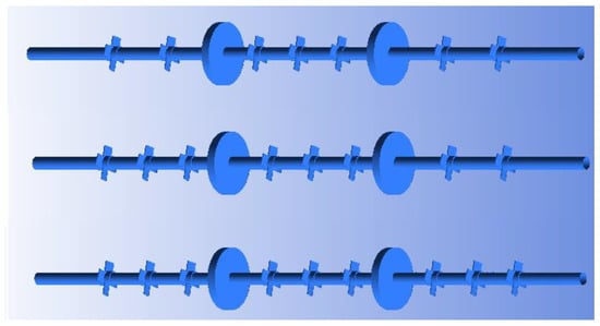
Figure 8.
Shaft with 7–9 impellers.
3.3. Finite-Element Analysis
For simulation purposes, the analysis used the Solidworks and Ansys software packages. Solidworks 2022, a computer-aided design (CAD) software package, was chosen for its ability to assemble components into complex systems. Ansys, a finite-element analysis (FEA) software package, was chosen for accurate calculations involving fluid–solid interaction (FSI). The detailed process of the simulation is represented by the flowchart in Figure 9.
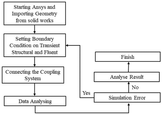
Figure 9.
Finite-element analysis flowchart.
The simulation process began by creating autoclave parts in Solidworks, followed by assembly and export to STEP format for use in Ansys. The subsequent procedure involved defining the boundary conditions in both the Transient Structural and Fluent modules within Ansys and establishing a coupling system to facilitate the exchange of data between the solid and fluid components. The simulation was then executed with thorough error checks. In the event of an error, the process reverted to the boundary-condition setup phase. If no errors were detected, analysis of the results, specifically those concerning bearing life, ensued. The accuracy of these results was subsequently confirmed through a comparison with data provided by the company. If the error margin remained below 10%, the simulation process was deemed complete; however, if it exceeded 10%, it reverted to the initial geometry construction phase. The FE models used in the simulation are illustrated in Figure 10.
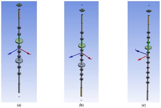
Figure 10.
FEA models (a) Seven impellers. (b) Eight impellers. (c) Nine impellers.
This study bifurcated the simulation into two distinct components: solid and liquid. The solid component was modeled through applying transient structures in Ansys, while the fluid component was represented through Fluent in Ansys. Moreover, to establish interaction between the solid and fluid portions, known as fluid–solid interaction (FSI), a coupling system was employed to establish a connection and facilitate the exchange of information between them. The mesh was partitioned into five distinct regions, each designed to balance precision with computational efficiency. These regions were named the Shaft and Impeller, the Tank, the Inner Diameter, the Ball and Roller, and the Outer Diameter. In the Boundary Condition (Transient) 1 section, various conditions were specified, including rotational velocity (to define the autoclave’s RPM), fixed support, thermal condition, and 12 FSI zones. FSI, which stands for fluid–solid interaction, was employed to regulate the exchange of information between specific zones or regions. The detailed statistics of finite elements and nodes are stated in Table 2.
Table 2.
FEA nodes and elements.
3.3.1. Boundary Condition (Solid)
The simulation of the solid part used the Transient Structural module of Ansys 2022 R2. The material used in this simulation was steel, which had the following material properties: a Young’s modulus of , a Poisson’s ratio of 0.3, a bulk modulus of , a shear modulus of , a compressive yield strength of , a tensile ultimate strength of , a tensile strength of , an isotropic thermal conductivity of , and a specific heat constant pressure of . A summary of the material properties is detailed in Table 3.
Table 3.
Material properties in the Transient Structural module in Ansys 2022 R2.
The boundary conditions for the solid part included fixed supports, rotational velocity, and fluid–solid interactions (FSIs). This transient section had 4 fixed supports, 1 rotational velocity, and 12 fluid–solid interactions (FSIs). Four fixed supports were located at the top of the NSK 732B bearing housing and at the bottom of the NSK 732B bearing housing. Two more were located where the shaft enters the tank of the autoclave. For rotational speed, the following settings were used: the coordinate system, namely, the global coordinate system, and the y component of 124.3 rad/s. For the fluid–solid interaction (FSI) settings in Ansys, there were 12 divisions, divided into 9 nine for the impeller, 2 for the disc, and 1 for the shaft. The full mesh used was 1,194,009.
3.3.2. Boundary Conditions (Fluid)
The simulation involved modeling the fluid section within the autoclave reactor using Ansys Fluent, employing a transient model. The initial phase involved identifying the flow type, achieved by calculating the Reynolds number (Re). Following the calculation of Re, the type of flow was found to be turbulent. Crucial configurations for the Ansys Fluent transient model involve activating the energy equation, employing a multiphase model mixture, and using the mass flow inlet as the inlet type, along with the pressure outlet for the outlet type. Two fluids, ethylene and vinyl acetate, were employed. Their specifications are as follows: the first was vinyl acetate, which has the chemical formula , a density of , a specific heat of , a thermal conductivity of , a viscosity of , a molecular weight of , and a standard state enthalpy of , while ethylene has the chemical formula , a density of , specific heat using the piecewise-polynomial equation, a thermal conductivity of , a viscosity of , a molecular weight of , and a standard state enthalpy of . The full mesh used was 2,575,856. A summary of the material details in Ansys fluent can be seen in Table 4.
Table 4.
Material properties for Ansys Fluent.
There were 10 zones in the cell zone conditions and 12 in the dynamic mesh. The 10 zones in the cell zone consisted of 9 rotating zones and 1 stationary zone, while the 12 zones in the dynamic mesh consisted of 9 impellers, 2 disks, and 1 shaft.
3.3.3. Fatigue-Life Calculation
Fatigue-life analysis in Ansys involves determining the endurance of a component under repeated loading until it fails due to material fatigue. Two methods are employed: stress life and strain life. Stress life utilizes an empirical S-N curve to establish the relationship between load intensity and the number of cycles before failure.
This study primarily focused on fatigue-life assessment using the stress-life method. To explain stress life, we relied on the S-N curve to determine the total number of cycles a bearing could withstand before failure. The objective of this study was to estimate the operational lifespan of bearings made from steel. The S-N curve of the bearing material is shown in Figure 11, and the stress with respect to a given number of cycles is shown in Table 5. Ansys software was employed to calculate a bearing’s fatigue life by evaluating the equivalent stress applied to the bearing, which was then correlated with the S-N curve to determine the number of cycles to failure. Subsequently, this number of cycles was divided by the daily operational cycles to estimate the bearing’s lifespan in days.
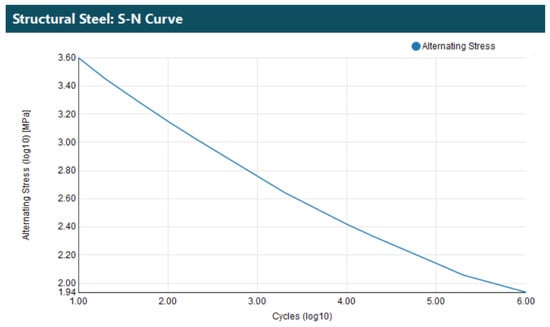
Figure 11.
S-N curve for steel in Ansys.
Table 5.
S-N curve table.
Ansys calculates fatigue life based on four key factors: the type of loading, the influence of mean stress, adjustments for multiaxial stress, and the application of a fatigue modification factor. Figure 12 illustrates the decision tree employed by Ansys to determine fatigue life when utilizing stress-life analysis.
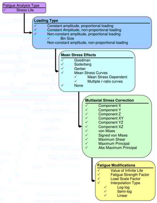
Figure 12.
Fatigue analysis (stress life) decision tree in Ansys.
This study focused on constant-amplitude full-reversed loading, where loads were applied and then reversed with equal magnitudes, simplifying the assessment. This approach relied on a single set of stress results and a loading ratio, assessing if the loads maintained a constant maximum value or varied continuously.
Mean stress effects were simulated using Goodman’s theory. Mean stress effects help manage the handling of the average stress effect. The average interval in this study was calculated using Goodman’s theory. The following equation is used for Goodman’s theory.
where is the stress and is the strength.
The simulation involved multiaxial stress correction through equivalent stress (von Mises). This approach, known as von Mises theory, is a fundamental concept in solid mechanics for predicting material yielding behavior. It simplifies complex three-dimensional stress states into a single positive stress value and is commonly employed in design work, particularly for ductile materials, to predict yielding based on maximum equivalent stress.
Fatigue adjustments are made through the utilization of the fatigue strength factor (Kf). This factor is integral to fatigue analysis, as it enables the customization of stress-life or strain-life curves by a designated factor. While the default value is set at 1, users have the flexibility to modify it either through manual input or by using a slider, with a range spanning from 0.01 to 1.
3.4. Optimization Using the Taguchi Method and the Response Surface Methodology
The problem of this study was and . Aside from that, the objective function of this study was to maximize , where bearing life, represented as “Y,” is the primary objective function. In this context, “Y” signifies the response specifically concerning bearing life, the variable “A” denotes the number of impellers, and “B” represents the temperature. Data analysis in this study leveraged various features within Minitab software, including Analyze Taguchi for response determination and S/N ratio graphing, Predict Taguchi for response prediction, Create a Response Surface Design for DOE creation, and Response Surface Design Analysis for response determination and analysis. The software’s capabilities extend to contour plots and surface plots to visualize factor relationships, and the Response Optimizer identifies optimal variable settings aligned with the study’s objectives of minimizing, targeting, or maximizing the response.
The optimization process using the Taguchi method is illustrated in Figure 13 through a flowchart outlining the optimization steps. Initially, a Design of Experiments (DOE) was created, employing an orthogonal array. In this case, the optimization problem entailed two factors (A and B) and 3 levels (1, 2, and 3), resulting in an orthogonal L9 array. Subsequently, response data were collected from each array. After gathering the data, analysis ensued, and the outcomes were organized in a table. To facilitate further examination, a signal-to-noise (S/N) ratio was graphically depicted. By analyzing the S/N ratio, the optimal parameters were determined. Once the optimal parameters were obtained for each method, additional experiments, in the form of simulations, were conducted to validate their representativeness as the optimal configuration. This was particularly crucial due to the potential non-integer nature of optimal parameter points, which can vary depending on the dataset used. The confirmatory experiments involved rerunning simulations with the optimal parameter data and comparing these results to the entire dataset to conclusively demonstrate that the identified parameters consistently yield superior outcomes. In the final stage, the confirmation of results was undertaken to ensure that the obtained response was genuinely the most optimal. If it was, the research concluded. If it was not, the process returned to the data collection stage for further refinement.
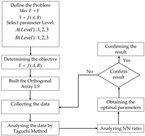
Figure 13.
Flowchart of optimization process using Taguchi method.
The flowchart in Figure 14 illustrates the optimization process using the response surface methodology, which commences with the Design of Experiments (DOE), specifically employing a central composite design. This DOE employed two factors, denoted A and B, with lower (L) and upper (U) limits defining the parameter range. Response data were then collected for each experimental run. After data collection, analysis ensued, employing the results from the response surface and Pareto chart data. The outcome of this analysis provided optimal parameters for each factor. Once the optimal parameters were derived for each method, additional experiments in the form of simulations were conducted to validate their representativeness as the optimal configuration. This validation was essential, considering the potential non-integer nature of optimal parameter points, which can vary depending on the dataset used. The confirmatory experiments entailed rerunning simulations with the optimal parameter data and comparing the results to the entire dataset to consistently demonstrate that these parameters yield superior outcomes. The final step involved ensuring that the response obtained was indeed optimal. If the results confirmed an optimal response, the research concluded. However, if they did not, the process reverted to the data collection stage for further refinement.
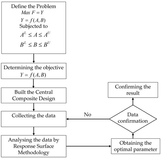
Figure 14.
Flowchart of optimization process using response surface methodology.
4. Results and Discussion
4.1. FEA Simulation Results
This study employed a simulation process to estimate the bearing life in an autoclave reactor. The simulation results, presented as contour plots, estimated that duration bearings can function reliably in the autoclave reactor before reaching failure due to repetitive loading. The minimum value on the contour plot represented the maximum bearing life before failure. The initial design involved nine impellers at a temperature of 150 °C. Bearing-life analysis was conducted for both mid and bottom bearings, and the bearing with the shortest estimated life was chosen as the response variable. The top bearing, a ball bearing of NSK 7322B type, was not analyzed as per the company’s data, indicating no damage. This omission aimed to expedite the simulation process. The bearing-life analysis results for the mid bearing (NSK 224M roller bearing) are illustrated in Figure 15a, while the results for the top bearing (FAG 224 roller bearing) can be seen in Figure 15b. The findings indicate that the mid bearings have an approximate lifespan of 80.043 days, while the bottom bearings have an estimated lifespan of 75.216 days. Since the bottom bearing has a shorter life compared to the mid bearing, it was chosen as the response value. Additionally, the obtained values for the bottom bearing with various parameters will be utilized to optimize the Taguchi and RSM methods.
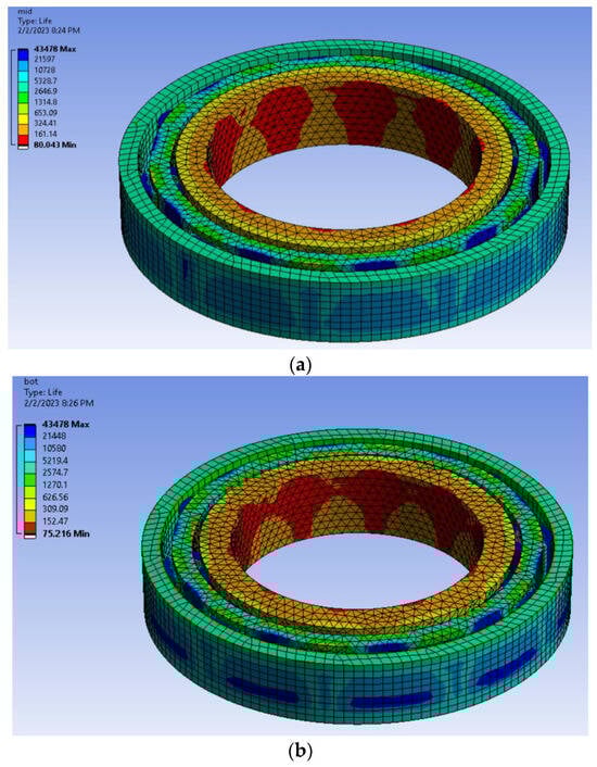
Figure 15.
FEA analysis of bearings. (a) Analysis of mid-bearing life. (b) Analysis of bottom-bearing life.
4.2. Optimization Using the Taguchi Method
The simulations were conducted using the L9 orthogonal array Design of Experiments (DOE) and the Taguchi method. Table 6 presents the factors and responses in the L9 orthogonal array, which consists of factors divided into three levels. Typically, the lowest value represents level 1, the median value represents level 2, and the highest value represents level 3. Minitab software calculated the bearing-life value using ANOVA with a 95% confidence level. Where a significant alpha value of 95% (α = 0.05) was used, it could be inferred that when the p-value was less than α, this indicated a significant influence of the factor on the response. Consequently, the analysis suggests that temperature is the only factor that significantly affects bearing life, whereas the impeller does not exhibit a significant impact. By examining the S/N ratio plot illustrated in Figure 16, it can be deduced that the primary factor influencing bearing life is temperature, followed by the number of impellers. Temperature exhibits a significant impact on the response, whereas the impeller does not hold much significance.
Table 6.
Taguchi method’s table of factors and responses using L9.
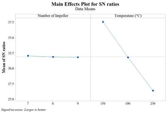
Figure 16.
S/N ratios from bearing-life main effect plot.
After examining the ANOVA table and the S/N ratio analysis, the ideal parameter values were determined. Subsequently, a tool called Predict Taguchi Result was employed to predict the bearing life based on these predetermined parameters. The outcome of this prediction represented the estimated bearing life under optimal conditions. In this case, the optimal configuration corresponded to seven blades and a temperature of 150 °C. According to the mean value, the bearing life was projected to be approximately 76.9957 days.
4.3. Optimization Using the Response Surface Methodology (RSM)
The experiments conducted involved simulations to acquire a response using the Design of Experiments (DOE) with a central composite design (CCD) matrix incorporating two factors. The summarized data in Table 7 present the factors and corresponding responses in relation to an autoclave reactor. The obtained results underwent analysis using the ANOVA technique with a 95% confidence level, facilitated by Minitab software. The inference drawn from this ANOVA, employing a significance level (alpha value) of 95% (α = 0.05), suggests that various factors including the number of impellers, temperature, the square of impellers, the square of temperature, and the correlation between impellers and temperature significantly impact bearing life. The significance of a factor is determined based on the comparison between its p-value and α. If the p-value is smaller than α, the factor is considered to have a significant influence, and vice versa.
Table 7.
RSM factors and responses using CCD.
The regression model employed in this analysis utilized a second-order approximation function known as the full squares regression model function. The regression equation representing bearing life (Y) is expressed in (4).
where A is the number of impellers and B is the temperature in the autoclave.
As per the Pareto chart depicted in Figure 17, the significance of each factor was determined, with Temperature (B) emerging as the most influential, followed by the square of the temperature (BB), the number of impellers (A), the square of the number of impellers (AA), and the correlation between the number of impellers and the temperature (AB) identified as the last factor impacting the response
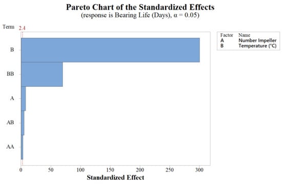
Figure 17.
Pareto chart for bearing life.
The contour plot in Figure 18a and the surface plot in Figure 18b demonstrated that the temperature range of 150–230 °C and a number of impellers between seven and nine contributed to improved bearing life. The optimal performance was achieved when the temperature was set at 150 °C with seven impellers.
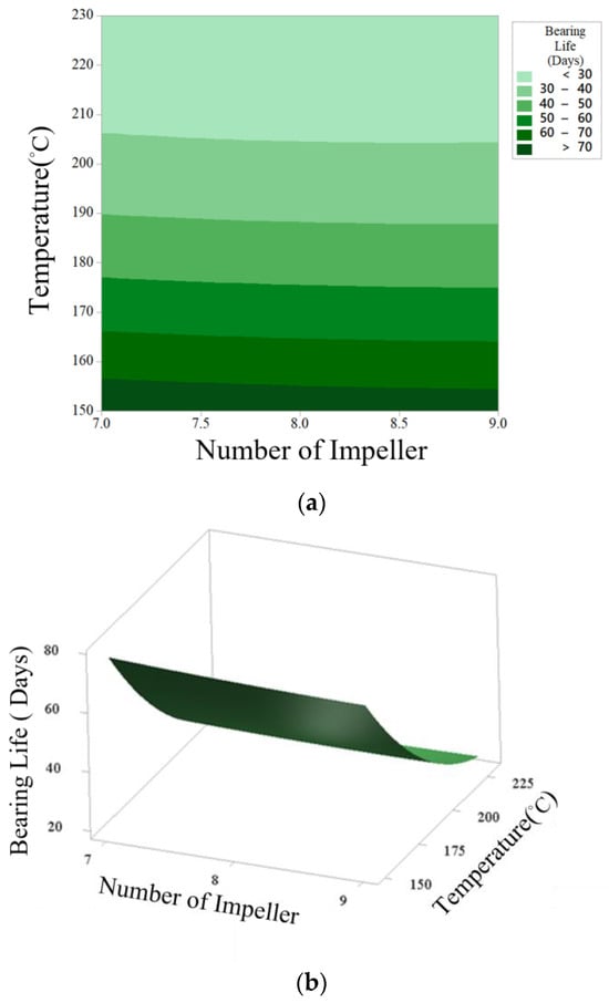
Figure 18.
Plot for bearing life and temperature with number of impellers. (a) Contour plot. (b) Surface plot.
To further optimize the autoclave reactor’s performance, response optimizer tools were employed. By maximizing the bearing life as the desired outcome, the response optimizer identified the most optimal parameters in the case of maximum bearing life when there are seven impellers and the temperature is 150 °C. These settings were estimated to result in a bearing life of 77.5854 days with a composite desirability of 1. The optimization plot in Figure 19 provides a visual representation of the installed values for the predictors of the optimal settings.
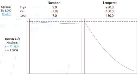
Figure 19.
Optimization plot from response optimizer using Minitab for bearing life.
4.4. Validation for Optimization Methods and Optimal Design
The prediction error was calculated to assess the performance of the optimization methods under optimal conditions. Comparing the prediction errors, the RSM method demonstrated better performance with 0.0533% in predicting bearing life compared to the Taguchi method with 0.707%.
The autoclave reactor optimization process used the TM, and the RSM had a variable number of impellers ranging from seven to nine and temperatures ranging from 150 to 230 °C. The optimal configuration involved seven impellers at a temperature of 150 °C, as determined by the optimization techniques. The resulting bearing life under these ideal conditions was 77.55 days. The increase in bearing life was calculated using equation 4 to quantify the improvement in bearing life achieved by the optimal design over the initial design. It can be inferred based on the calculation that the optimal design exhibits a 3.095% increase in bearing life compared to the initial design.
5. Conclusions
This study aimed to optimize an autoclave reactor system for maximum bearing life by analyzing simulation data validated through experimental data from the company to obtain its fatigue life. Data optimization was conducted using the Taguchi method, which utilized ANOVA and S/N ratio plots to determine the significance of factors, while the response surface methodology relied on Pareto charts, ANOVA tables, and regression equations. Both methods yielded the same optimal parameters: seven impellers and a temperature of 150 °C. However, they differed in identifying the influential factors, with the TM highlighting only temperature as significant, while the RSM identified the number of impellers and the temperature as significant factors. Further, regarding response prediction (bearing life), the Taguchi method had a prediction error of 0.70708%, while the RSM outperformed it with a prediction error of 0.0534%, such that it is better suited for analyzing intricate relationships between factors and responses, leading to more accurate predictions with a 95% confidence level. Ultimately, the optimized variables resulted in a 3.095% increase in bearing life compared to the initial design, leading to cost savings and reduced downtime. Future research can focus on expanding the parameters studied for autoclave reactor optimization and bearing-life improvement, exploring control strategies and real-time monitoring systems, and integrating advanced optimization algorithms.
Author Contributions
Conceptualization, P.T.L. and C.-L.C.; methodology, P.T.L. and H.-Y.L.; software, F.F. and B.P.; formal analysis, H.-C.C. and S.-J.P.; investigation, F.F. and H.-C.C.; writing—original draft preparation, B.P.; writing—review and editing, B.P. and P.T.L.; visualization, P.T.L. and C.-L.C.; supervision, P.T.L. and H.-Y.L.; funding acquisition, P.T.L. All authors have read and agreed to the published version of the manuscript.
Funding
The support from the National Science and Technology Council (NSTC), Taiwan (grant numbers NSTC 112-2221-E-002-001, MOST 111-2221-E-002-001, and MOST 110-2221-E-002-022), and the Intelligent Manufacturing Innovation Center (IMIC), which is a Featured Areas Research Center in Higher Education Sprout Project of the Ministry of Education (MOE), Taiwan, was appreciated.
Data Availability Statement
The data presented in this study are available on request from the corresponding author. The data are not publicly available due to privacy.
Conflicts of Interest
The authors declare no conflict of interest.
References
- Sivalingam, G.; Soni, N.J.; Vakil, S.M. Detection of decomposition for high pressure ethylene/vinyl acetate copolymerization in autoclave reactor using principal component analysis on heat balance model. Can. J. Chem. Eng. 2015, 93, 1063–1075. [Google Scholar] [CrossRef]
- You, D.; Feron, D.; Turluer, G. Experimental simulation of low rate primary coolant leaks. For the case of vessel head penetrations affected by through wall cracking. In Proceedings of the International Conference on Water Chemistry in Nuclear Reactors Systems–Operation Optimisation and New Developments, Avignon, France, 22–26 April 2002. [Google Scholar]
- Kumar, V. Multivariate Statistical Monitoring of a High-Pressure LDPE and EVA Copolymer Industrial Process. Ph.D. Thesis, University of Alberta, Alberta, 2002. [Google Scholar]
- Turman, E.; Strasser, W. CFD modeling of LDPE autoclave reactor to reduce ethylene decomposition: Part 2 identifying and reducing contiguous hot spots. Chem. Eng. Sci. 2022, 257, 117722. [Google Scholar] [CrossRef]
- Heinonen, M. LDPE Reactor Mixer Bearing Faults. Brüel & Kjær Vibro Megazine. 2013. Available online: https://www.bkvibro.com/wp-content/uploads/2020/12/LDPE_REACTOR_MIXER_BEARING_FAULTS_en_ext.pdf (accessed on 20 January 2023).
- Albdery, M.H.; Szabó, I. A Review of Fault Diagnosis Techniques of Rolling Element Bearings for Rotating Machinery. Int. J. Sci. Technol. Res. 2021, 10, 170–174. [Google Scholar]
- Li, K.; Wang, Q. Study on signal recognition and diagnosis for spacecraft based on deep learning method. In Proceedings of the 2015 Prognostics and System Health Management Conference (PHM), Beijing, China, 21–23 October 2015; pp. 1–5. [Google Scholar]
- Nabhan, A.; Ghazaly, N.; Samy, A.; Mousa, M.O. Bearing fault detection techniques-a review. Turk. J. Eng. Sci. Technol. 2015, 3, 1–18. [Google Scholar]
- Jammu, N.; Kankar, P. A review on prognosis of rolling element bearings. Int. J. Eng. Sci. Technol. 2011, 3, 7497–7503. [Google Scholar]
- Brandolin, A.; Sarmoria, C.; Lótpez-Rodríguez, A.; Whiteley, K.S.; Del Amo Fernández, B. Prediction of molecular weight distributions by probability generating functions. Application to industrial autoclave reactors for high pressure polymerization of ethylene and ethylene-vinyl acetate. Polym. Eng. Sci. 2001, 41, 1413–1426. [Google Scholar] [CrossRef]
- Wang, Y.; Liu, C.; Wang, S.; Dong, H. Investigation on flow characteristic and reaction process inside an EVA autoclave reactor using CFD modeling combined with polymerization kinetics. Korean J. Chem. Eng. 2022, 39, 1384–1395. [Google Scholar] [CrossRef]
- Torotwa, I.; Ji, C.Y. A study of the mixing performance of different impeller designs in stirred vessels using computational fluid dynamics. Designs 2018, 2, 10. [Google Scholar] [CrossRef]
- Chien, I.-L.; Kan, T.W.; Chen, B.-S. Dynamic simulation and operation of a high pressure ethylene-vinyl acetate (EVA) copolymerization autoclave reactor. Comput. Chem. Eng. 2007, 31, 233–245. [Google Scholar] [CrossRef]
- Pladis, P.; Kanellopoulos, V.; Baltsas, A.; Kiparissides, C. Dynamic Modeling and Optimization of Flash Separators for Highly-Viscous Polymerization Processes. In Computer Aided Chemical Engineering; Elsevier: Amsterdam, The Netherlands, 2011; Volume 29, pp. 723–727. [Google Scholar]
- Hamzaçebi, C.; Li, P.; Pereira, P.; Navas, H. Taguchi Method as a Robust Design Tool. In Quality Control-Intelligent Manufacturing, Robust Design and Charts; IntechOpen: London, UK, 2020. [Google Scholar]
- Myers, R.H.; Montgomery, D.C.; Anderson-Cook, C.M. Response Surface Methodology: Process and Product Optimization Using Designed Experiments; John Wiley & Sons: Hoboken, NJ, USA, 2016. [Google Scholar]
- Zhou, J.; Wu, D.; Guo, D. Optimization of the production of thiocarbohydrazide using the Taguchi method. J. Chem. Technol. Biotechnol. 2010, 85, 1402–1406. [Google Scholar] [CrossRef]
- Bello, E.I.; Ogedengbe, T.I.; Lajide, L.; Daniyan, I.A. Optimization of Process Parameters for Biodiesel Production Using Response Surface Methodology. Am. J. Energy Eng. 2016, 4, 8. [Google Scholar] [CrossRef]
- Said, K.A.M.; Amin, M.A.M. Overview on the Response Surface Methodology (RSM) in Extraction Processes. J. Appl. Sci. Process. Eng. 2015, 2, 8–17. [Google Scholar] [CrossRef]
- Liang, C.-G.; Li, H.; Hao, B.; Ma, P.-C. Optimization on the performance of fibrous filter through computational fluid dynamic simulation coupled with response surface methodology. Chem. Eng. Sci. 2023, 280, 119070. [Google Scholar] [CrossRef]
- Lu, C.; Liu, S. Contact Fatigue Reliability Analysis of Rolling Bearing based on Elastohydrodynamic Lubrication. Int. J. Perform. Eng. 2020, 16, 855–865. [Google Scholar]
- Henderson, A.M. Ethylene-vinyl acetate (EVA) copolymers: A general review. IEEE Electr. Insul. Mag. 1993, 9, 30–38. [Google Scholar] [CrossRef]
- Maurya, A.K.; Mishra, A.; Mishra, N. Nanoengineered polymeric biomaterials for drug delivery system. In Nanoengineered Biomaterials for Advanced Drug Delivery; Elsevier: Amsterdam, The Netherlands, 2020; pp. 109–143. [Google Scholar]
- Bearing Life–Calculating the Basic Fatigue Life Expectancy of Rolling Bearings. A Publication of Nsk Europe. Available online: https://www.nskeurope.com/content/dam/nskcmsr/downloads/literature_bearing/P_TI-0102_EN.pdf (accessed on 20 January 2023).
- Lee, Y.; Jeon, K.; Cho, J.; Na, J.; Park, J.; Jung, I.; Park, J.; Park, M.J.; Lee, W.B. Multicompartment Model of an Ethylene–Vinyl Acetate Autoclave Reactor: A Combined Computational Fluid Dynamics and Polymerization Kinetics Model. Ind. Eng. Chem. Res. 2019, 58, 16459–16471. [Google Scholar] [CrossRef]
- Zadghaffari, R.; Moghaddas, J.; Revstedt, J. A mixing study in a double-Rushton stirred tank. Comput. Chem. Eng. 2009, 33, 1240–1246. [Google Scholar] [CrossRef]
- Hassan, I.T.M.; Robinson, C.W. Stirred-tank mechanical power requirement and gas holdup in aerated aqueous phases. AIChE J. 1977, 23, 48–56. [Google Scholar] [CrossRef]
Disclaimer/Publisher’s Note: The statements, opinions and data contained in all publications are solely those of the individual author(s) and contributor(s) and not of MDPI and/or the editor(s). MDPI and/or the editor(s) disclaim responsibility for any injury to people or property resulting from any ideas, methods, instructions or products referred to in the content. |
© 2023 by the authors. Licensee MDPI, Basel, Switzerland. This article is an open access article distributed under the terms and conditions of the Creative Commons Attribution (CC BY) license (https://creativecommons.org/licenses/by/4.0/).