Application of Stochastic Resonance for Detection of Weak Signals in Electromagnetic Systems

Abstract

This article presents a comprehensive analytical, numerical, and experimental study of the amplification and detection of weak signals in magnetically coupled electromagnetic systems, using an architecture consisting of three magnetically coupled coils. A rigorous mathematical model of the system is developed, which includes the formulation of the mutual inductance matrix and a state-space representation that captures the dynamic interaction between the coils. It is important to note that the electromagnetic subsystem is linear and that the stochastic resonance effect is achieved by incorporating an external nonlinear bistable element. In this configuration, a weak periodic signal below a threshold is applied to the primary coil, while a controlled source of Gaussian white noise is injected into a secondary coil. A third coil functions as a sensing element, capturing the superimposed magnetic response resulting from coupling effects. The voltage induced in the sensor coil is subsequently processed by a bistable nonlinear element implemented via a Schmitt trigger, which provides the nonlinearity and bistability necessary to enable stochastic resonance and the detection of the weak periodic signal. The conditions of the SR are analyzed in terms of noise intensity, coupling coefficients, and system parameters, highlighting the existence of an optimal noise level that maximizes the signal-to-noise ratio (SNR) at the output. A detailed simulation framework has been developed in MATLAB/Simulink, enabling a systematic exploration of the parameter space and the validation of theoretical predictions. The simulation results are further supported by experimental measurements obtained from a physical prototype, which show agreement with the proposed model. The main contribution of this work lies in demonstrating that magnetically coupled electromagnetic structures can effectively interact with nonlinear bistable elements to exploit stochastic resonance in the detection of weak signals, even when the electromagnetic domain itself remains linear. The results demonstrate that magnetic coupling is an effective mechanism for mediating constructive interactions between noise and weak signals, thereby improving the detection of the latter. These results extend the applicability of stochastic resonance to hybrid electromagnetic systems and demonstrate its relevance in practical applications. Potential applications include ultra-sensitive magnetic detection, low-power signal detection, magnetic transducers, and robust signal recovery in noisy electromagnetic environments, particularly in contexts where conventional linear amplification fails.

1. Introduction

The concept of stochastic resonance (SR) was first introduced in the early 1980s by Benzi, Sutera, and Vulpiani, who proposed that the quasi-periodic recurrence of Earth’s glacial cycles could be explained by the constructive interaction between weak periodic orbital forcing and environmental noise within a nonlinear climate system [1]. This pioneering work challenged the conventional paradigm that noise is inherently detrimental, demonstrating instead that random fluctuations can enhance system performance under appropriate conditions. In this context, stochastic resonance describes a counterintuitive phenomenon in which the presence of an optimal level of noise maximizes the response of a nonlinear system to a weak periodic input signal, enabling its detection or transmission even when it lies below the system’s activation threshold. Since its introduction, SR has been extensively explored in various fields, such as Physics [2,3], Biology [4], Medicine [5,6], Mechanical Systems [7], Signal Processing [8,9,10] and Image Processing [11]. Noise-assisted enhancement has enabled improved detection capabilities. From a theoretical standpoint, SR is typically observed in nonlinear bistable systems, in which noise induces transitions between potential wells, leading to synchronization between the system’s switching dynamics and the external periodic excitation.

In recent years, increasing attention has been devoted to the application of stochastic resonance in magnetic systems, particularly in the context of weak signal detection. For instance, stochastic resonance has been successfully applied to magnetic anomaly detection (MAD), where weak magnetic signals buried in strong background noise can be enhanced using bistable, tristable, or multistable nonlinear systems [12,13,14]. Advanced configurations such as parallel stochastic resonance systems and compound tristable models have demonstrated significant improvements in signal-to-noise ratio and detection probability, even under extremely low input SNR conditions. These approaches highlight the practical relevance of SR in electromagnetic sensing applications [15,16,17,18].

Furthermore, stochastic resonance has also been experimentally observed in electronic and electromagnetic platforms, including chaotic circuits [19,20,21] used for the detection of weak periodic magnetic field signals, where noise-induced transitions enhance the system response at specific frequencies [19]. In addition, studies have explored the role of magnetic flux in modulating stochastic resonance behavior in nonlinear oscillatory systems, demonstrating that electromagnetic coupling and flux-dependent dynamics can significantly influence signal-to-noise characteristics and system coherence [22]. These findings suggest that electromagnetic interactions can play an active role in shaping stochastic resonance phenomena beyond purely abstract models.

In the context of magnetic sensing and imaging, stochastic resonance has also been exploited to enhance signals derived from magnetic resonance systems, such as MRI, where controlled noise injection improves image quality and feature detectability [23]. This further supports the idea that noise-assisted techniques are not only theoretically relevant but also practically viable in electromagnetic-based technologies.

Despite the broad interdisciplinary impact of stochastic resonance, its application to physically coupled electromagnetic systems—particularly those involving energy transfer via mutual inductance—remains relatively unexplored. While previous work has largely focused on nonlinear dynamical systems or signal processing frameworks, fewer studies have addressed architectures in which the electromagnetic coupling itself mediates the interaction between noise and weak signals.

Therefore, although important progress has been made in magnetic signal detection using stochastic resonance, there is still a lack of systematic studies that investigate how magnetically coupled electromagnetic structures can be integrated with nonlinear processing elements to exploit stochastic resonance in a controlled and physically interpretable manner. This knowledge gap was the motivation for this work, whose objective is to explore stochastic resonance in an architecture of multiple magnetically coupled coils, providing both a theoretical framework and experimental validation for weak signal enhancement assisted by a Gaussian white noise signal.

2. Materials and Methods

2.1. Mathematical Model of Coupled Inductors

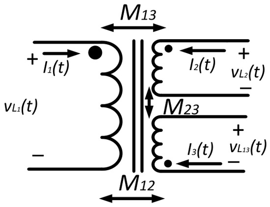
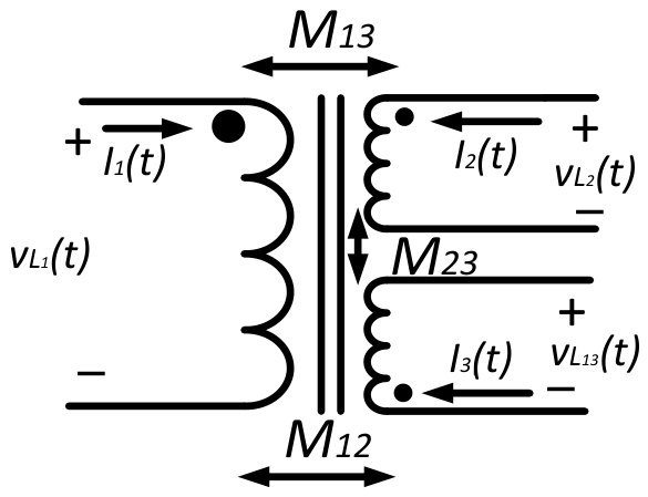
Figure 1 illustrates an electromagnetic system consisting of three magnetically coupled coils, which forms the physical basis for analyzing energy transfer and nonlinear phenomena in multilayer structures. Each coil is characterized by its own inductance and by the currents flowing through it, i₁(t), i₂(t) and i₃(t) (See arrow directions and coupling points) while the interactions between them are modeled using mutual inductance, M₁₂, M₁₃ and M₂₃ (See the up and down arrows). These mutual inductances represent the degree of magnetic coupling between each pair of coils. This type of configuration is particularly relevant for the study of phenomena such as wireless power transfer; coupled circuits; and, in the context of this work, the possible emergence of effective nonlinear behaviors when the system is subjected to weak excitations and stochastic perturbations. The interaction between multiple coupled inductors can generate conditions equivalent to multistable systems, opening the possibility of analyzing mechanisms such as stochastic resonance in electromagnetic domains.

The electrical dynamics of the system can be formulated in the time domain using a set of coupled differential equations, in which the voltage across each coil is expressed as a function of its self-inductance, mutual inductances, and external excitation sources. The resulting formulation, presented in the system of Equation (1), provides a complete description of the electrical interactions in the time domain and serves as the basis for subsequent analysis, simulation, and experimental validation of the SR phenomenon in the proposed architecture.

$$\begin{array}{l}{v}_{L_1}(t)=L_1{\displaystyle \frac{d{i}_1(t)}{dt}}+M_{12}{\displaystyle \frac{d{i}_2(t)}{dt}}+M_{13}{\displaystyle \frac{d{i}_3(t)}{dt}}\\ v_{L_2}(t)=M_{21}{\displaystyle \frac{d{i}_1(t)}{dt}}+L_2{\displaystyle \frac{d{i}_2(t)}{dt}}+M_{23}{\displaystyle \frac{d{i}_3(t)}{dt}}\\ v_{L_3}(t)=M_{31}{\displaystyle \frac{d{i}_1(t)}{dt}}+M_{32}{\displaystyle \frac{d{i}_2(t)}{dt}}+L_3{\displaystyle \frac{d{i}_3(t)}{dt}}\end{array}$$

(1)

where L₁, L₂ and L₃ are the inductances of the coupled coils and M₁₂, M₁₃, M₂₁, M₂₃, M₃₁ and M₃₂ are the mutual inductances between the three coils. Due to the reciprocity of Maxwell’s laws, the coupling between coils is identical in both directions, so M₁₂ = M₂₁, M₁₃ = M₃₁ and M₂₃ = M₃₂. Mutual inductances are calculated using Equation (2). The instantaneous currents flowing through the coils are defined as i₁, i₂ and i₃. While the applied voltages are $v_{L_1}(t)$, $v_{L_2}(t)$ and $v_{L_3}(t)$,

$$M_{ij}=k_{ij}\sqrt{L_i{L}_j}$$

(2)

where $M_{ij}$ represents the mutual inductance between inductors i and j. The system of equations shown in Equation (1) describes the dynamic coupling between the three inductors and can be compactly expressed in matrix form as Equation (3).

$$v=L{\displaystyle \frac{di}{dt}}$$

(3)

where $v={\left[v_{L_1} v_{L_2} v_{L_3}\right]}^T$ is the voltage vector, $i={\left[i_1 i_2 i_3\right]}^T$ is the current vector and $L$ is the inductance matrix defined as shown in Equation (4).

$$L=\left[\begin{array}{ccc}{L}_1& M_{12}& M_{13}\\ M_{12}& L_2& M_{23}\\ M_{13}& M_{23}& L_3\end{array}\right]$$

(4)

2.2. Mathematical Model of Stochastic Resonance

The theoretical description of stochastic resonance is commonly formulated using a bistable nonlinear system driven by both deterministic and stochastic excitations. Such systems are typically modeled using stochastic differential equations derived from the Langevin formalism [24]. A classical representation of a bistable system is given by a particle moving in a double-well potential. The dynamics of the particle can be described by the overdamped Langevin equation. This is shown in Equation (5).

$${\displaystyle \frac{dx}{dt}}=-{\displaystyle \frac{U(x)}{dx}}+A\cos (\omega t)+\sqrt{2D}\xi (t)$$

(5)

where x is the state variable of the system (position of the particle), and Acos(ωt) is the weak periodic signal (the input). It is “weak” because its amplitude A is too small to cause the system to jump over the potential barrier on its own. $-{\displaystyle \frac{U(x)}{dx}}$ is the derivative of the bistable potential (double well), and D denotes the noise intensity. The term $\xi (t)$ represents Gaussian white noise with zero meaning and autocorrelation.

$$U(x)=-{\displaystyle \frac{a}{2}}{x}^2+{\displaystyle \frac{b}{4}}{x}^4$$

(6)

where a and b are positive constants that determine the shape of the potential, with two wells of minimum energy separated by a barrier of maximum energy at x = 0. This potential has two stable equilibrium points located at Equation (7).

$$x=\pm \sqrt{{\displaystyle \frac{a}{b}}}$$

(7)

Separated by an unstable equilibrium point at x = 0, which corresponds to the potential barrier, the deterministic force acting on the particle is obtained from the potential gradient shown in Equation (8).

$${\displaystyle \frac{-dU\left(x\right)}{dx}}=ax-b{x}^3$$

(8)

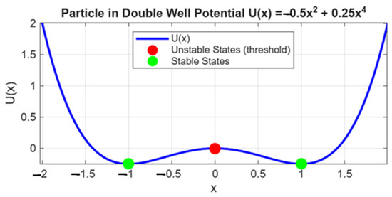
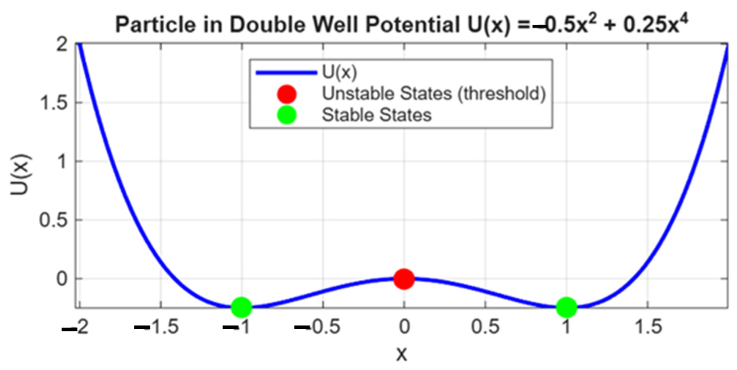
In the absence of noise, a weak periodic signal with amplitude smaller than the barrier height is generally insufficient to induce transitions between the two stable states, and the system remains confined within a single potential well. However, when stochastic perturbations are introduced, random fluctuations may provide the necessary energy for the particle to overcome the potential barrier. Figure 2 presents a double-well potential, described by the function $U(x)=-{\displaystyle \frac{a}{2}}{x}^2+{\displaystyle \frac{b}{4}}{x}^4$, which is a classic case in the analysis of nonlinear and bistable systems. The shape of the curve shows two symmetric minima located approximately at x = −1 and x = 1, as well as a maximum at x = 0. This geometry defines an energy landscape in which a particle can be located. From a physical standpoint, the potential minimum corresponds to stable equilibrium states, since small perturbations around these points tend to bring the system back to them. In contrast, the central point x = 0 is an unstable equilibrium, since any perturbation, no matter how small, will cause the particle to fall into one of the two potential wells. This point acts as an energy barrier separating the two stable states.

2.3. Mathematical Model of a Schmitt Trigger

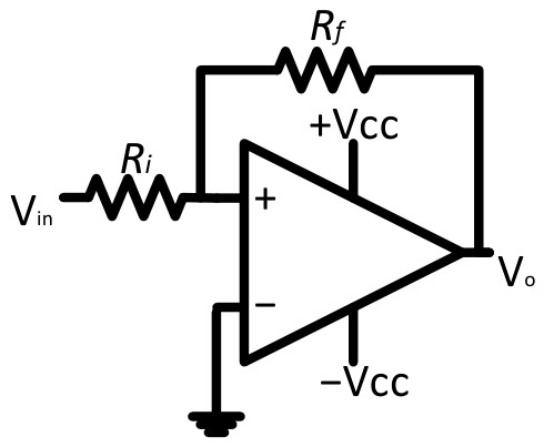
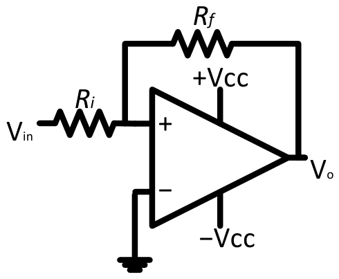
A Schmitt trigger is a nonlinear comparator circuit (see Figure 3) characterized by the presence of hysteresis, which introduces two distinct switching thresholds and thus defines a bistable system. This hysteretic behavior ensures that the output does not switch at a single threshold level but rather depends on the variation in the input signal. Let v_in be the input voltage, v_o the output voltage, R_f the feedback resistance, and Ri the input resistance. From the perspective of dynamical systems, the Schmitt trigger can be interpreted as an electronic implementation of a bistable potential, analogous to a particle evolving in a double-well energy landscape (see Figure 2). In this analogy, the comparator’s two stable output states (high and low) correspond to the minimum of the potential wells, while the switching thresholds define an effective energy barrier separating these states. The positive feedback introduced by R_f is responsible for creating this bistability, as it reinforces the current state of the system and requires a sufficiently large disturbance at the input to induce a transition to the opposite state.

The switching behavior of the circuit is governed by two threshold voltages: the upper threshold V_TH and the lower threshold V_TL, with $V_{TH}>V_{TL}$. The output of the Schmitt trigger switches between two saturation levels $+V_{sat}$ and $-V_{sat}$ depending on the value of the signal relative to these thresholds. The operation of the Schmitt trigger can be described by the piecewise nonlinear function shown in Equation (9).

$$V_o(t)=\left\{\begin{array}{l}+V_{sat}, v_{in}(t)\ge V_{TH}\\ -V_{sat}, v_{in}(t)\le V_{TL}\\ V_o(t^{-}), V_{TL}<v_{in}(t)<V_{TH}\end{array}\right\}$$

(9)

where $V_o(t^{-})$ represents the previous state of the output. This condition reflects the hysteresis property of the circuit, where the output remains in its current state until the input crosses one of the switching thresholds. The thresholds are determined by the feedback network of the circuit. For a Schmitt trigger implemented with an operational amplifier and a resistive feedback network, the upper and lower thresholds are shown in Equations (10) and (11).

$$V_{TH}=\beta V_{sat}$$

(10)

$$V_{TL}=-\beta V_{sat}$$

(11)

where β is the feedback factor determined by the resistive network composed of R_i and R_f. This parameter defines the fraction of the output voltage that is fed back to the input, thereby directly setting the switching thresholds of the Schmitt trigger. In particular, the value of β establishes the width of the hysteresis band, since both the upper and lower threshold levels are proportional to the output saturation voltage scaled by this feedback factor. This is shown in Equation (12).

$$\beta ={\displaystyle \frac{R_i}{R_i+R_f}}$$

(12)

When the input signal includes stochastic fluctuations, the total excitation applied to the system can be modeled as the superposition of a deterministic component and a random process. In this case, the input voltage is typically expressed as the sum of a weak periodic signal representing the information of interest and a stochastic term accounting for noise, often modeled as Gaussian white noise with zero mean and finite variance. This representation allows the influence of random disturbances on the system’s dynamics to be captured in a mathematically manageable way. This is shown in Equation (13).

$$V_{in}\left(t\right)=\mathrm{s}\left(t\right)+\mathrm{n}\left(t\right)$$

(13)

where s(t) represents a deterministic signal and n(t) is a noise process. In this case, noise may induce transitions between the two stable output states when the combined signal crosses the switching thresholds. This mechanism allows the Schmitt trigger to behave as a bistable nonlinear system, making it suitable for the study of SR phenomena.

2.4. Mathematical Equivalence Between a Double-Well Potential and a Schmitt Trigger

The mathematical connection between a double-well potential, the Langevin equation, and a Schmitt trigger lies in the concepts of bistability and hysteresis. These three concepts represent the same physical/mathematical phenomenon modeled at different levels of abstraction: from continuous statistical physics (Langevin equation and bistable double-well system) to macroscopic discrete electronics (Schmitt trigger). Their most common point of convergence is the study of SR.

A Schmitt trigger is an electronic circuit that has two stable states (high and low) and exhibits hysteresis. It does not change state immediately in response to the input but rather has two distinct voltage thresholds: one for switching on (V_TH) and another for switching off (V_TL). The Mathematical Bridge analyzing the Langevin system without noise ξ(t) = 0 is shown in Equation (14).

$${\displaystyle \frac{-dU(x)}{dx}}=ax-b{x}^3+F(t)$$

(14)

If we assume that the signal F(t) changes very slowly (quasi-static condition), the system always seeks equilibrium: −dU(x)/dx = 0. See Equation (15).

$$ax-b{x}^3=F(t)$$

(15)

For small forces F(t), the cubic equation has three roots (two stable ones corresponding to the wells, and one unstable one). However, if the force F(t) increases, the double-well potential “tips over.” A critical point will be reached, where one of the potential wells disappears completely. To find this point, we differentiate the restoring force with respect to x and set it equal to zero:

$${\displaystyle \frac{d}{dx}}\left(ax-b{x}^3\right)=a-3b{x}^2=0\to x_c=\sqrt{{\displaystyle \frac{a}{3b}}}$$

(16)

By replacing these critical points x_c and substituting this back into the force equation, we obtain the exact external force required to destroy one well and force the system to jump to the other:

$$F_c=\pm \sqrt{{\displaystyle \frac{4a^3}{27b}}}$$

(17)

The critical force (F_c) of the Langevin continuous system corresponds mathematically to the threshold voltages of a Schmitt trigger.

$$V_{TH}=+\sqrt{{\displaystyle \frac{4a^3}{27b}}}$$

(18)

$$V_{TL}=-\sqrt{{\displaystyle \frac{4a^3}{27b}}}$$

(19)

When the noise ξ(t) is reintroduced into the system (the full case of the Langevin equation), the particle can jump between the wells before the external force F(t) reaches the critical thresholds F_c. This is governed by the Kramers rate. In applications such as SR, rather than numerically solving the computationally expensive continuous stochastic differential equation, the continuous Langevin system is simplified or “mapped” to a discrete two-state model. Mathematically, the continuous variable x(t) is passed through an asymmetric function that mimics the behavior of the bifurcation:

$$y(t)=\mathrm{sgn}(x(t))$$

(20)

From a macroscopic modeling perspective, injecting a noisy signal F(t) + ξ(t) into a Langevin equation with a double-well potential will produce an output x(t) whose abrupt transitions are mathematically identical to injecting that same noisy signal into the input of a Schmitt trigger. In summary: The Schmitt trigger is the discrete-time and discrete-state abstraction of the nonlinear dynamics experienced by a particle in a double-well potential modeled by the Langevin equation.

3. Results

This section will present the theoretical, simulation, and experimental results of the application of stochastic resonance in electromagnetic systems.

3.1. Theoretical Results

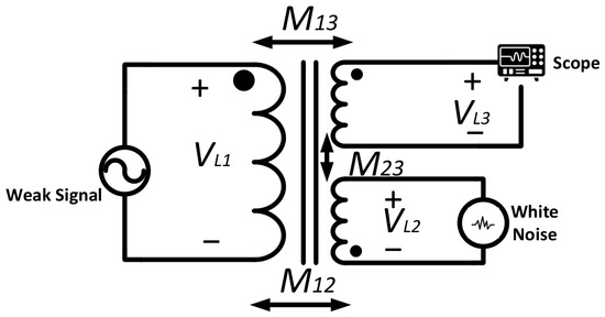
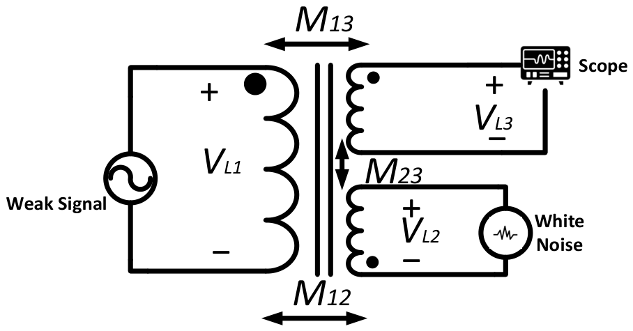
Consider a system of three coupled inductors (See Figure 4). L₁ is fed with a low-amplitude sinusoidal source (weak signal). L₂ is fed with a Gaussian white noise generator with a defined power spectral density, and L₃ will be the “sensor” inductor that will measure the interaction between the white noise and the weak signal.

Taking the system of differential equations shown in (1) and the system proposed in Figure 4, L₃ is connected to an oscilloscope, which has an impedance in the order of MΩ, so L₃ is in an open circuit; therefore, ${\displaystyle \frac{d{i}_3(t)}{dt}}\approx 0$ and the system of equations are simplified and shown in Equation (21).

$$\begin{array}{l}{v}_{L_1}(t)=L_1{\displaystyle \frac{d{i}_1}{dt}}+M_{12}{\displaystyle \frac{d{i}_2}{dt}}\\ v_{L_2}(t)=M_{21}{\displaystyle \frac{d{i}_2}{dt}}+L_2{\displaystyle \frac{d{i}_2}{dt}}\\ v_{L_3}(t)=M_{31}{\displaystyle \frac{d{i}_1}{dt}}+M_{32}{\displaystyle \frac{d{i}_2}{dt}}\end{array}$$

(21)

To formalize the dynamics of the coupled-coil system, the system of algebraic equations is transformed into a standard representation in state space, defined by the standard canonical form of the matrix. This is shown in Equation (22):

$$\begin{array}{l}\dot{x}(t)=Ax(t)+Bu(t) \\ y(t)=Cx(t)+Du(t)\end{array}$$

(22)

First, the system vectors are defined. The state vector x(t) consists of the currents in the primary and secondary inductors; the input vector u(t) contains the excitation voltages applied to these coils; and the output vector y(t) corresponds to the voltage induced in the sensor coil. See Equation (23).

$$x(t)=\left[\begin{array}{c}{i}_1(t)\\ i_2(t)\end{array}\right], u(t)=\left[\begin{array}{c}{v}_{L_1}(t)\\ v_{L_2}(t)\end{array}\right], y(t)=V_{L_3}(t)$$

(23)

Using the matrix equations for the inverse of inductance, we can define the state equation. Since the current model considers ideal inductors and does not include series resistances (parasitic or load), the state of the current derivatives depends purely on the voltage inputs and not on the current states. Therefore, the state matrix A is a zero matrix, and the input matrix B is defined by the inductance parameters. This is shown in Equation (24).

$$\dot{x}(t)=\left[\begin{array}{cc}0& 0\\ 0& 0\end{array}\right]\left[\begin{array}{c}{i}_1(t)\\ i_2(t)\end{array}\right]+{\displaystyle \frac{1}{\Delta }}\left[\begin{array}{cc}{L}_2& -M_{12}\\ -M_{12}& L_1\end{array}\right]\left[\begin{array}{c}{v}_{L_1}(t)\\ v_{L_2}(t)\end{array}\right]$$

(24)

where $∆=L_1{L}_2-M_{12}^2$. For the output equation, the voltage across the third coil VL₃(t) depends on the exchange rates of the flows i₁ and i₂. When substituting the equation of state $\dot{x}$ into the output equation, we see that the output depends directly on the input vector u(t) scaled by the magnetic couplings, without direct dependence on the states x(t). Thus, we obtain matrices C and D. This is shown in Equation (25).

$$y(t)=\left[\begin{array}{cc}0& 0\end{array}\right]\left[\begin{array}{c}{i}_1(t)\\ i_2(t)\end{array}\right]+{\displaystyle \frac{1}{\Delta }}\left[M_{31}{L}_2-M_{32}{M}_{12}-M_{31}{M}_{12}+M_{32}{L}_1\right]\left[\begin{array}{c}{v}_{L_1}(t)\\ v_{L_2}(t)\end{array}\right]$$

(25)

This matrix representation (A, B, C, D) fully captures the linear dynamic behavior of the electromagnetic subsystem, serving as the theoretical basis for the subsequent injection into the Schmitt trigger.

According to Maxwell’s reciprocity laws, the coupling M₁₂ is equal to M₂₁, so Equation (21) can be rewritten in matrix form and is shown in Equation (26).

$$\left[\begin{array}{l}{v}_{L_1}\\ v_{L_2}\end{array}\right]=\left[\begin{array}{cc}{L}_1& M_{12}\\ M_{12}& L_2\end{array}\right]\left[\begin{array}{c}{\displaystyle \frac{d{i}_1}{dt}}\\ {\displaystyle \frac{d{i}_2}{dt}}\end{array}\right]$$

(26)

The inductance matrix is inverted to calculate the derivatives of currents i₁ and i₂. This is shown in Equation (27).

$$\left[\begin{array}{c}{\displaystyle \frac{d{i}_1}{dt}}\\ {\displaystyle \frac{d{i}_2}{dt}}\end{array}\right]={\displaystyle \frac{1}{L_1{L}_2-{M_{12}}^2}}\left[\begin{array}{cc}{L}_2& -M_{12}\\ -M_{12}& L_1\end{array}\right]\left[\begin{array}{l}{v}_{L_1}\\ v_{L_2}\end{array}\right]$$

(27)

The derivatives of currents i₁ and i₂ are calculated from the matrix expression (27). This is shown in Equation (28).

$$\begin{array}{l}{\displaystyle \frac{d{i}_1}{dt}}={\displaystyle \frac{1}{\Delta }}\left(L_2{v}_{L_1}(t)-M_{12}{v}_{L_2}(t)\right)\\ {\displaystyle \frac{d{i}_2}{dt}}={\displaystyle \frac{1}{\Delta }}\left(-M_{12}{v}_{L_1}(t)+L_1{v}_{L_2}(t)\right)\end{array}$$

(28)

where the Δ term is equivalent to Equation (29).

$$\Delta =L_1{L}_2-{M_{12}}^2$$

(29)

Substituting (28) for $v_{L_3}(t)$ shown in Equation (21), we obtain Equation (30):

$$v_{L_3}(t)=M_{31}{\displaystyle \frac{1}{\Delta }}\left(L_2{v}_{L_1}-M_{12}{v}_{L_2}\right)+M_{32}{\displaystyle \frac{1}{\Delta }}\left(-M_{12}{v}_{L_2}+L_2{v}_{L_1}\right)$$

(30)

Factoring for $v_{L_1}(t)$ (weak periodic signal) and $v_{L_2}(t)$ (Gaussian white noise signal), the voltage across L₃ is expressed in Equation (31).

$$v_{L_3}(t)={\displaystyle \frac{1}{L_1{L}_2-{M_{12}}^2}}\left[\left(M_{31}{L}_2-M_{32}{M}_{12}\right)\left(v_{L_1}(t)\right)+\left(-M_{31}{M}_{12}+M_{32}{L}_1\right)\left(v_{L_2}(t)\right)\right]$$

(31)

A computational algorithm was developed in MATLAB ^® (2024b) to evaluate and visualize the dynamic voltage responses of the three coupled coils. This algorithm is based on the numerical solution of Equation (31) derived from the magnetic circuit model. The algorithm calculates the instantaneous voltages across each inductor, $v_{L_1}(t)$ and $v_{L_2}(t)$. These voltages are stored and processed to generate time-domain plots, allowing for a direct visualization of the interaction between the weak signal, the Gaussian white noise, and the signal observed at the L₃ sensor coil.

These values for each inductor and mutual inductance are shown in

Table 1. Inductor values and coupling coefficients.

Element	Description	Value
L1	Inductor 1	1 mH
L2	Inductor 2	1 mH
L3	Inductor 3	1 mH
k12	Coupling Coefficient of L1 to L2	0.9
k13	Coupling Coefficient of L1 to L3	0.9
K23	Coupling Coefficient of L2 to L3	0.9

.

Using Equation (2), the mutual inductances are calculated; the results are shown in Equations (32)–(34).

$$M_{12}=k_{12}\sqrt{L_1{L}_2}=9\times {10}^{-4}$$

(32)

$$M_{13}=k_{13}\sqrt{L_1{L}_3}=9\times {10}^{-4}$$

(33)

$$M_{23}=k_{23}\sqrt{L_2{L}_3}=9\times {10}^{-4}$$

(34)

To systematically evaluate the effect of SR on the system’s response, this study considers three distinct scenarios. First, a reference case is analyzed in which no noise is injected into the system, allowing the response to be evaluated solely in terms of the weak periodic signal. Second, an intermediate case is examined in which the noise level is set to an optimal value, where SR is expected to occur and the detectability of the weak signal is maximized. Finally, a third scenario with excessive noise is evaluated, in which the stochastic component dominates the system dynamics and degrades signal quality. This comparative approach clearly identifies the constructive role of noise and provides evidence that SR exists in magnetically coupled systems. For the first case study (without noise), the values shown in

Table 2. Noise signal and weak signal (no noise) parameters.

Element	Description	Value
D	Power Spectral Density	0 V2/Hz
A	Weak Signal Amplitude	30 mV
f	Weak Signal Frequency	60 Hz
fs	Sampling Frequency	150 kHz
ts	Sampling Time	6.666 µS

are proposed.

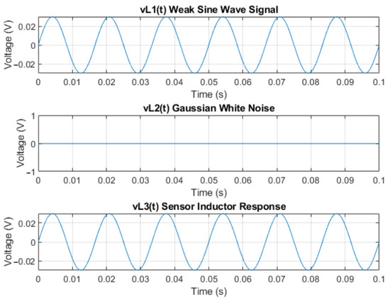
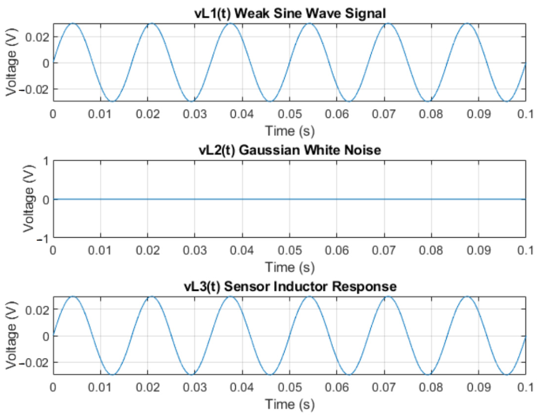
Figure 5 shows the theoretical results. The top signal shows the weak periodic signal (60 Hz, 30 mVp), and the middle signal shows a total absence of noise, meaning the spectral power density is equal to 0 V²/Hz. The bottom signal shows the response of the sensor coil, which is the response obtained in Equation (31).

A new power spectral density is defined again to re-evaluate Equation (31) with the parameters shown in Table 1 and

Table 3. Gaussian white noise parameters and weak periodic signal.

Element	Description	Value
D	Power Spectral Density	1 × 10−9 V2/Hz
A	Weak Signal Amplitude	30 mV
f	Weak Signal Frequency	60 Hz

, leading to the formulations presented in Equations (32)–(34). This procedure corresponds to the second case under analysis, in which the noise level is adjusted to an optimal value. In this regime, the stochastic component is expected to constructively interact with the weak periodic signal, promoting noise-assisted transitions and maximizing the system response, thereby enabling the observation of stochastic resonance.

Figure 6 shows the responses of the three inductors. The top graph shows the weak signal with a maximum amplitude of 30 mV at a frequency of 60 Hz. The middle graph shows the white Gaussian white noise with the power spectral density shown in Table 3. The bottom graph shows the response of the sensing coil, which corresponds to that obtained from Equation (31) in the time domain. This signal can cross defined thresholds, and thus, the phenomenon of stochastic resonance can occur.

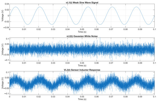
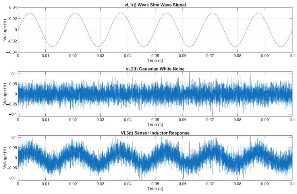
Equation (31) is now evaluated for the third case of study, in which the system is subjected to an excessive noise level, while maintaining the same set of parameters used in the previous scenarios. In this condition, the stochastic component dominates the system dynamics, leading to a degradation in the coherence between the input periodic signal and the output response. The corresponding power spectral density for this regime is presented in

Table 4. Parameters of weak and noise signals (excessive noise).

Element	Description	Value
D	Power Spectral Density	9 × 10−9 V2/Hz
A	Weak Signal Amplitude	30 mV
f	Weak Signal Frequency	60 Hz

, allowing a direct comparison with the previous cases and highlighting the detrimental effect of high noise intensity on signal detectability.

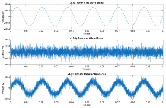
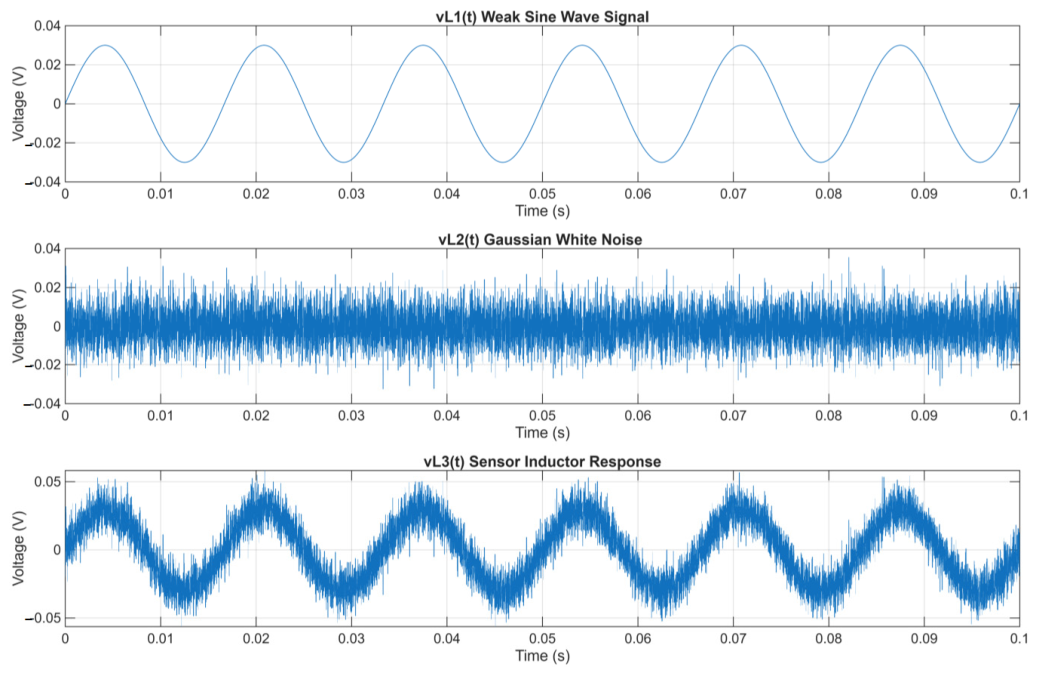
Figure 7 shows the responses of the three inductors. The top graph shows the weak signal (60 Hz, 30 mVp). The middle graph shows the white Gaussian noise with a power spectral density of 9 × 10⁻⁹ V²/Hz, which is excessive. The bottom graph shows the response of the sensing coil, which corresponds to the value obtained in Equation (31). This signal can cross a defined threshold many times, resulting in a completely chaotic response in a bistable system.

3.2. Simulation Results

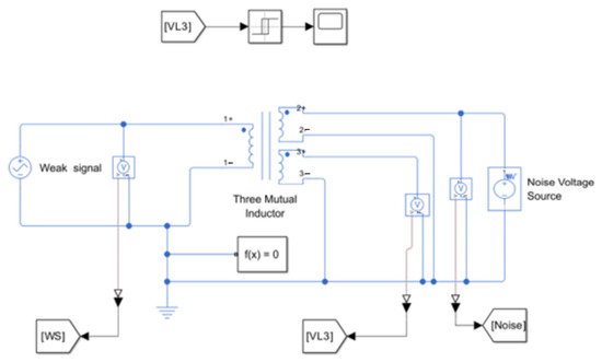
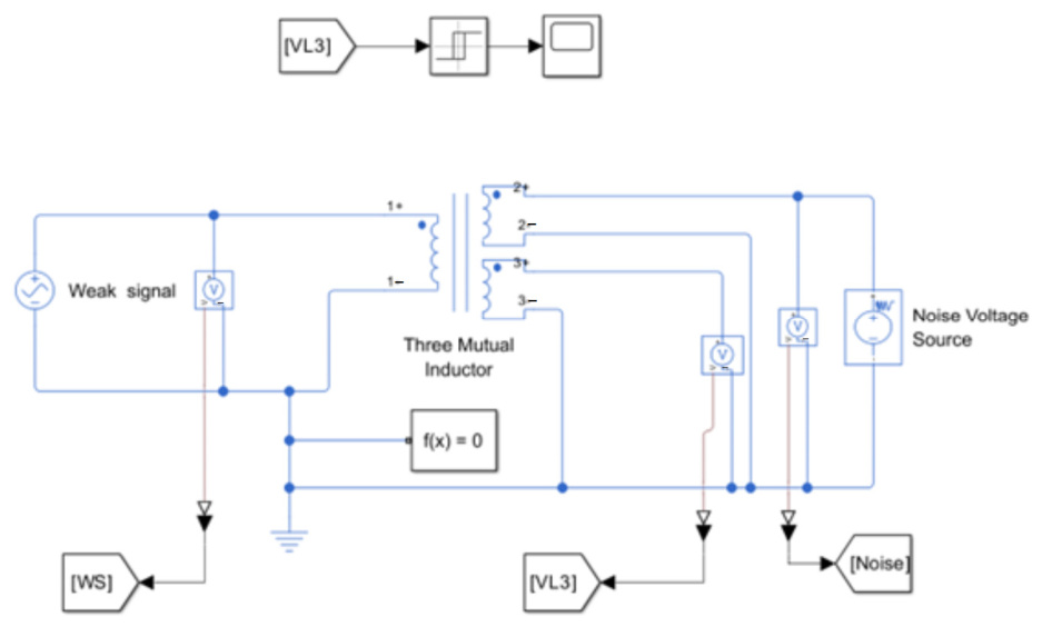
Figure 8 shows a Simulink^® model using the Simscape library of an electromagnetic system based on three magnetically coupled inductors, as shown in Figure 4. On the left side of the circuit is the periodic weak signal source, which excites the system’s primary winding. This low-amplitude signal alone might not be sufficient to generate a significant response in the system. The signal is monitored using a voltage measurement block and sent to an oscilloscope for visualization. The core of the system consists of a “Three Mutual Inductor” block, which models three coils coupled via mutual inductance. This block represents the magnetic coupling between the windings, enabling energy transfer between them.

The top part of the model includes the relay block, which mathematically models the hysteresis of a Schmitt trigger, thereby representing a bistable system with a defined activation threshold. On the right side, a Gaussian White Noise source is incorporated, which is fed into one of the coupled windings. This source is essential for analyzing how the noise interacts with the weak signal through magnetic coupling. This source allows the spectral power density to be varied. Overall, the model will allow us to analyze how a weak signal can be detected through the interaction of Gaussian white noise within a magnetically coupled system. This type of setup is particularly relevant for the study of nonlinear systems, weak signal detection, and phenomena such as stochastic resonance. The values for the inductive components and the sources were taken from Table 1, Table 2, Table 3 and Table 4.

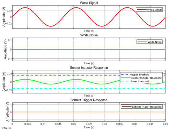
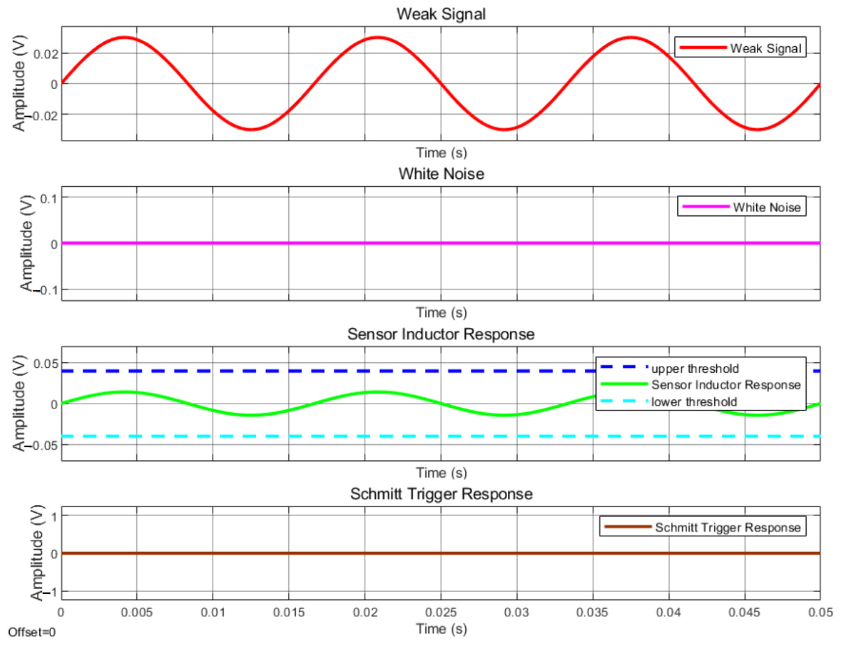
Figure 9 shows the following. The red signal represents the weak signal with an amplitude of 30 mV at a frequency of 60 Hz. The pink signal indicates that coil 2 is not being fed with the white Gaussian noise signal; that is, there is no noise. The green signal shows the response of the sensor coil (coil 3). The maximum and minimum amplitudes are below the defined thresholds of ±40 mV (dark blue and light blue signals). Because of this, the Schmitt trigger response is 0 V (brown signal) since its input signal (green signal) does not exceed the trigger thresholds.

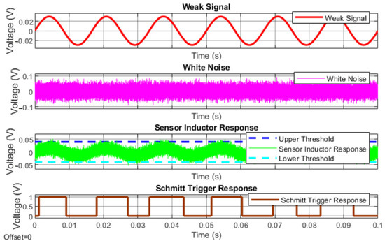
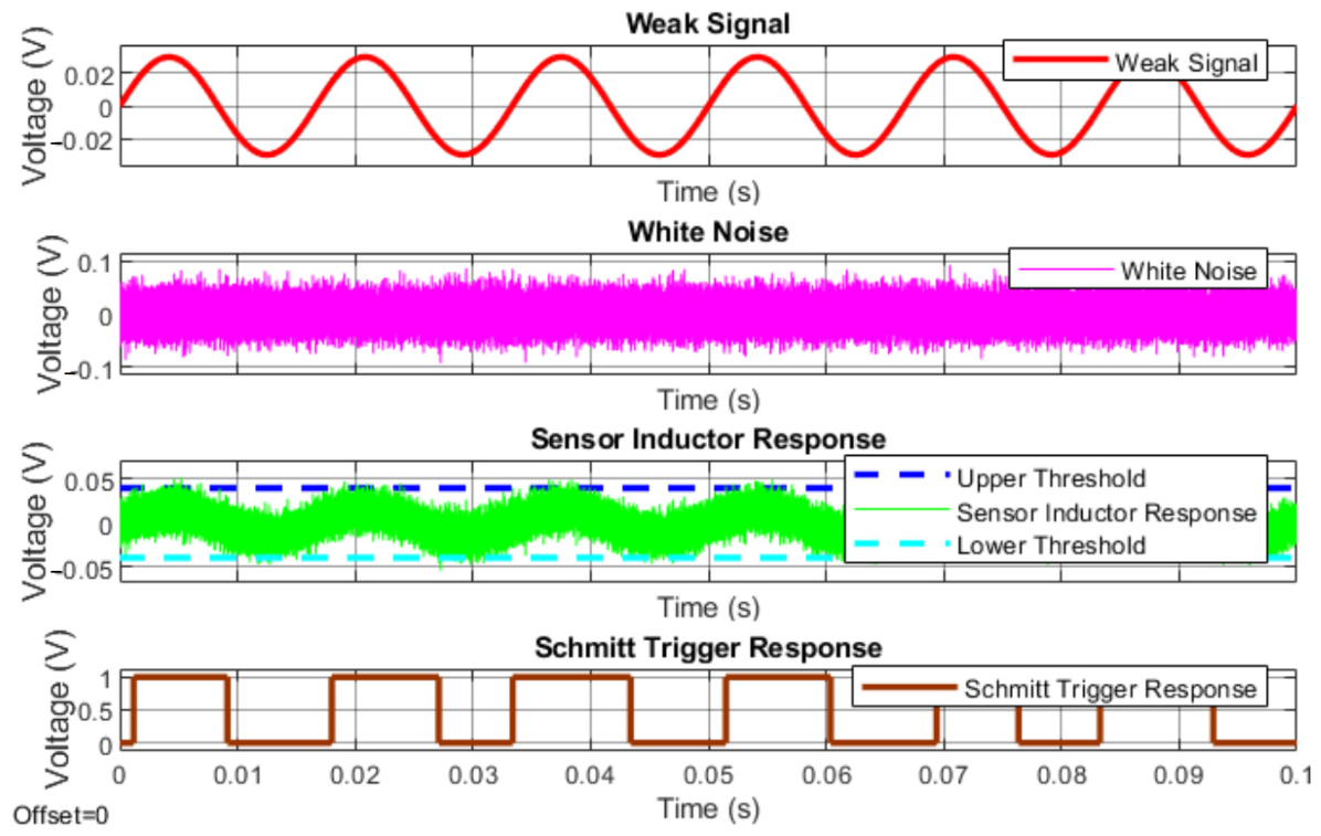
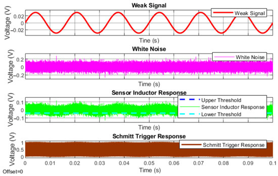
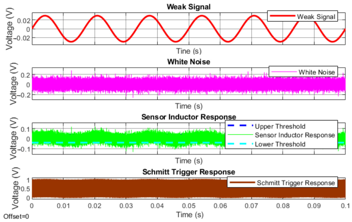
Figure 10 shows the following. The red signal represents the weak signal with an amplitude of 30 mV at a frequency of 60 Hz. The pink signal represents the voltage of coil 2, which is fed with a white Gaussian noise signal. The green signal represents the response of the sensor coil. The maximum and minimum amplitudes exceed the defined thresholds of ±40 mV (dark blue and light blue signals). Because of this, the response of the bistable system (Schmitt trigger) synchronizes with the frequency of the weak signal (see brown signal), thus confirming the occurrence of stochastic resonance in electromagnetic systems. This is due to the addition of an optimal amount of noise, which improved the electromagnetic detection of the weak signal.

Figure 11 shows the following: the red signal represents the weak signal. The pink signal represents the voltage of L₂, fed with a white Gaussian noise signal. The green signal represents the response of the L₃ coil. The maximum and minimum amplitudes exceed the defined thresholds of ±40 mV on multiple occasions. Because of this, the Schmitt trigger response becomes completely chaotic (see the brown signal) due to excessive noise (D = 6 × 10⁻⁹ V²/Hz), as the signal-to-noise ratio is not suitable for stochastic resonance to occur.

3.3. Signal-to-Noise Ratio

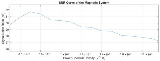
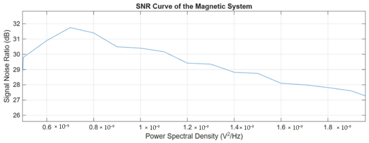
To evaluate the performance of the proposed magnetic system, an analysis of the signal-to-noise ratio (SNR) was conducted on the system’s output signal (Schmitt trigger output). The SNR was used as the primary metric to quantify the system’s ability to amplify weak signals embedded in noise. The SNR was calculated using Equation (35).

$$SNR=10{\log }_{10}\left({\displaystyle \frac{P_{signal}}{P_{noise}}}\right)$$

(35)

where P_signal represents the power of the spectral component corresponding to the weak input signal, and P_noise corresponds to the average power of the noise in the spectrum. Figure 12 shows the SNR curve obtained for different noise levels applied to the system. For power spectral density values below 0.5 V²/Hz, the SNR cannot be determined because the Schmitt trigger does not activate. The weak signal does not have enough energy to exceed the system’s threshold. As the noise power spectral density increases from 0.5 V²/Hz, the SNR rises progressively until it reaches a maximum peak, a phenomenon characteristic of stochastic resonance.

This behavior indicates that there is an optimal noise level capable of maximizing the transfer of energy from the weak signal to the system output. Beyond this optimal point, a further increase in noise causes the SNR to decrease because the noise begins to dominate the system dynamics and degrades the detectability of the useful signal.

3.4. Experimental Results

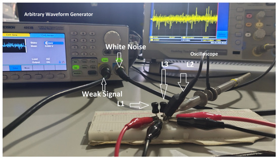
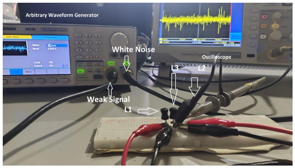
To validate the theoretical formulation and numerical predictions presented in the previous sections, an experimental setup has been developed to demonstrate the occurrence of stochastic resonance in a system of three magnetically coupled coils. The objective of this phase is to demonstrate, under real operating conditions, the constructive interaction between a weak periodic signal and a stochastic excitation controlled via electromagnetic coupling, as well as to quantify its effect on signal detectability. The experimental setup (see Figure 13) replicates the architecture shown in Figure 4, in which the first coil is driven by a low-amplitude sinusoidal source representing the weak signal, the second coil is driven by a Gaussian noise generator with an adjustable power spectral density, and the third coil functions as a sensing element. The voltage induced in the sensor coil is acquired using appropriate measurement instruments with sufficient bandwidth. The objective was to demonstrate that the presence of noise can improve the system’s response to a weak periodic input signal and synchronize a bistable system.

Table 5. Electrical characteristics of the coils.

Frequency	Description	Value
60 Hz	Parasitic resistance	5.11 Ω
1 KHz	Parasitic resistance	12.93 Ω
60 Hz	Inductance	0.996 mH
1 KHz	Inductance	0.999 mH

shows the electrical characteristics of the coils used in the experimental prototype, which were obtained using an LCR meter.

The following are the experimental responses of the electromagnetic system under three different noise conditions, no noise, optimal noise and excess noise, thus illustrating the fundamental mechanism of stochastic resonance. The 40 mVp threshold was determined based on previous experimental tests, which showed that at this level, the sensor coil’s response was the minimum sufficient to prevent the signal from being distorted or interfered with by external noise.

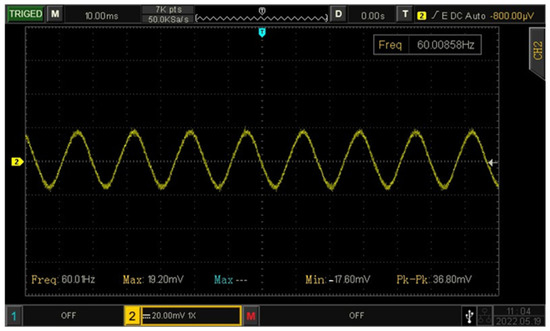
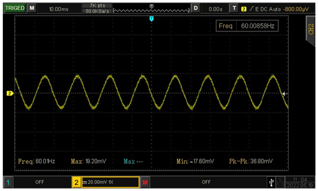
Figure 14 shows the output signal of L₃ in the absence of external noise. Under these conditions, the weak periodic excitation (60 Hz) is insufficient to induce transitions in the system, resulting in a low-amplitude response (19.20 mV max, −17.60 mV min and 36.80 mVpp). The signal remains confined and does not exhibit significant switching behavior, indicating that the system operates below the activation threshold (±40 mV).

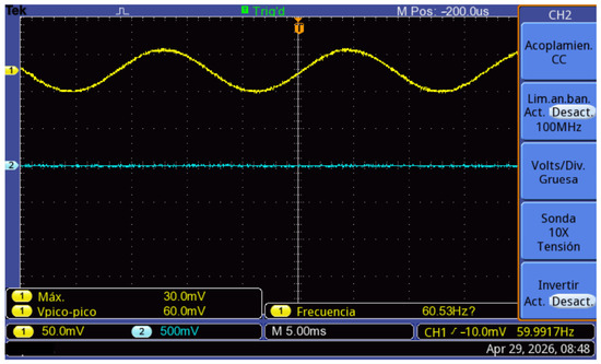
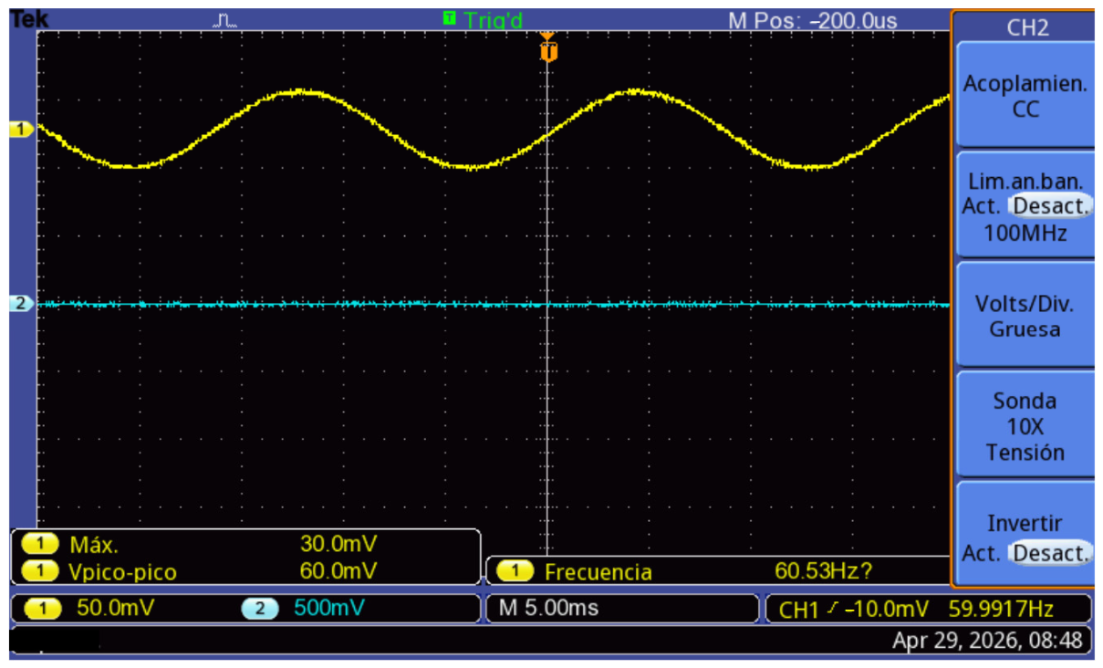
Figure 15 shows the weak sinusoidal signal in yellow. For this test, it has a peak-to-peak voltage of 60 mV and a peak-to-peak amplitude of 30 mV; this signal is still too weak for the Schmitt trigger to detect, so it does not produce any response (blue signal).

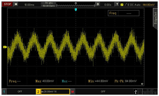
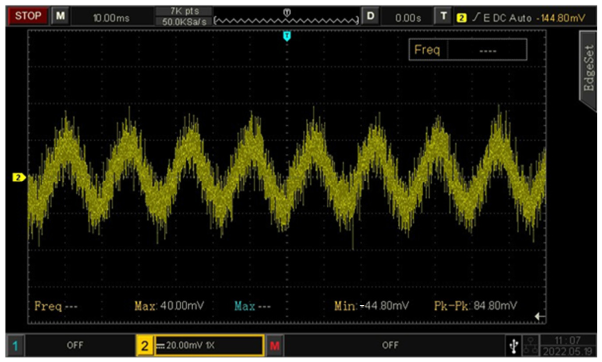
In Figure 16, an optimal noise level is introduced into the system. The response of coil L₃ is significantly improved (40 mV max, −44.80 mV min and 84.80 mVpp), and the output signal exhibits clear transitions synchronized with the input excitation (60 Hz in the fundamental frequency). This behavior is a direct manifestation of stochastic resonance, where the constructive interaction between the noise and the weak periodic signal allows the system to overcome the potential barrier (±40 mV). As a result, the signal becomes detectable enough to perform the synchronized transitions in a Schmitt trigger.

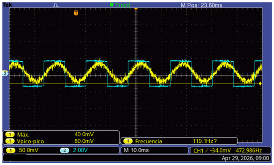
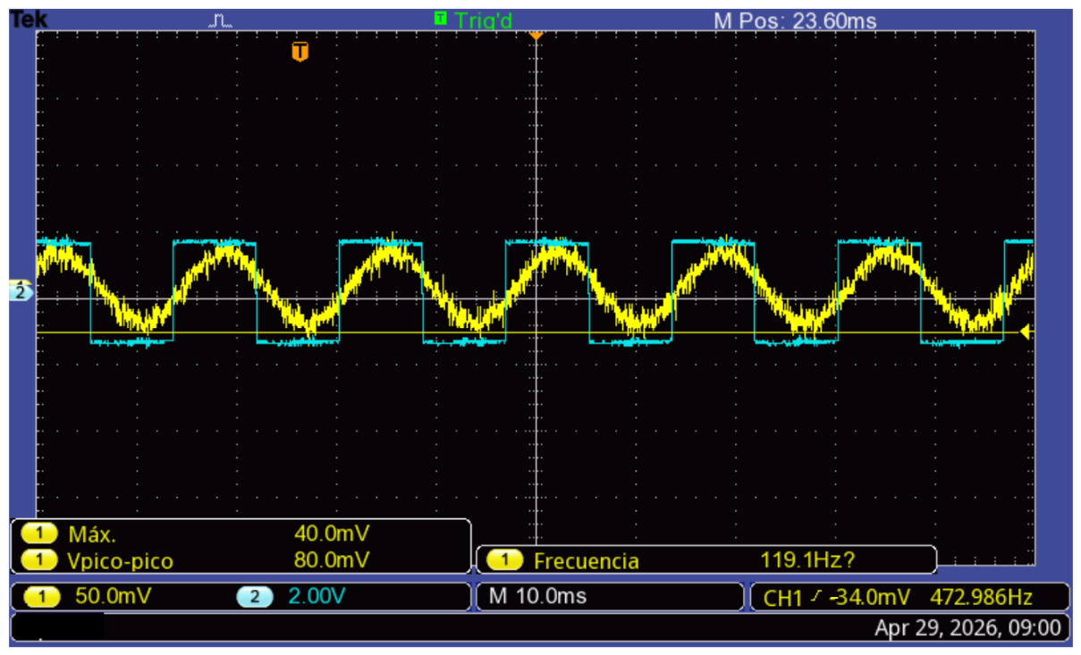
Figure 17 shows the weak sinusoidal signal interacting with Gaussian white noise (yellow signal). For this test, the signal has a maximum voltage of 40 mV, which is the trigger threshold; therefore, the response of the Schmitt trigger (blue signal) synchronizes with the fundamental frequency of the weak signal (60 Hz), thus causing the phenomenon of stochastic resonance in a magnetic system.

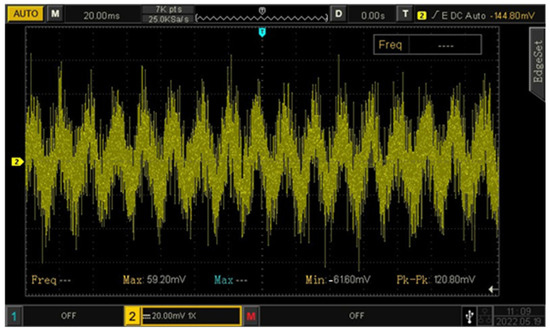
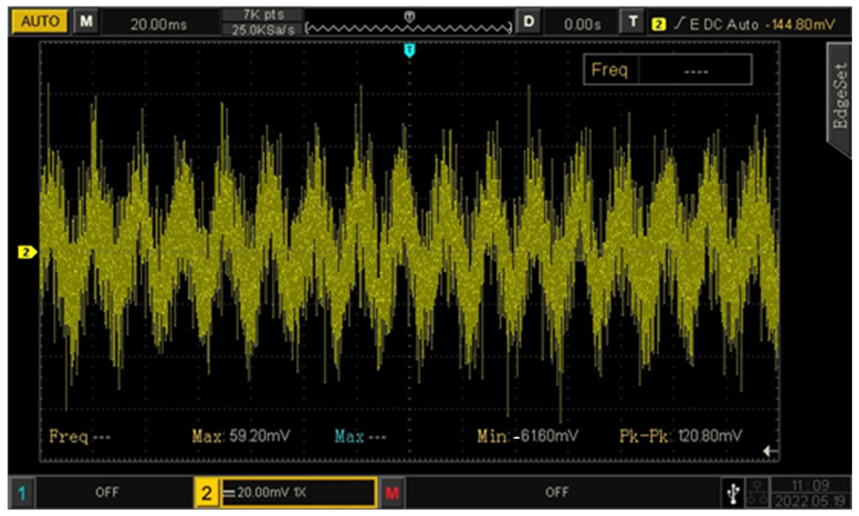
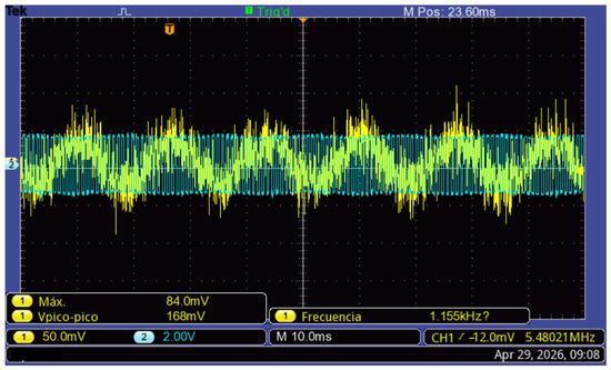
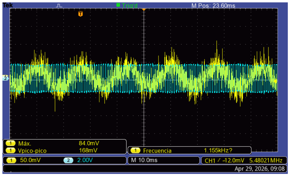
In contrast, Figure 18 shows the system’s response under excessive noise conditions. In this case, the output signal becomes irregular and dominated by random fluctuations (See Figure 18). The underlying periodic component is no longer distinguishable, indicating that the beneficial effect of noise is lost when its intensity exceeds the optimum level. The signal shows a maximum peak of 59.20 mV, a minimum peak of −61.60 mV, and a peak-to-peak voltage of 120.80 mV. Although the ±40 mV threshold is well exceeded, the signal is overwhelmed by the noise, resulting in a chaotic response at the Schmitt trigger.

Figure 19 shows the interaction between the weak signal and excessive noise (yellow signal). In this test, the signal has a peak voltage of 84 mV, which far exceeds the trigger threshold; therefore, the response of the Schmitt trigger (blue signal) becomes desynchronized from the fundamental frequency of the weak signal and becomes chaotic.

The experimental results presented in this section provide clear evidence of the feasibility of achieving noise-assisted signal enhancement in a system of three magnetically coupled coils. The measurements confirm that the interaction between a weak periodic excitation and a controlled stochastic input can be effectively transferred via electromagnetic coupling and observed in the sensor coil, thereby validating the theoretical framework presented in the Introduction section. The observed trends are consistent with both the analytical model and the simulations, which supports the validity of the proposed approach. Overall, these findings demonstrate that stochastic resonance can be successfully achieved in electromagnetic systems, not just in the areas traditionally studied. This opens the door to practical applications in weak signal detection, magnetic detection, and signal recovery in noisy environments.

4. Discussion

Compared to previous studies, the observed behavior is consistent with the classical theory of stochastic resonance [2], originally developed for climate models [1,25,26,27] and later extended to mechanical [28], electronic [29,30,31], and biological systems [32]. In these studies, stochastic resonance is characterized by the synchronization of noise-induced transitions with a weak periodic excitation, leading to an enhanced system response to a specific noise level.

However, studies on magnetic systems are very scarce [13,19,33]. In [19], the stochastic resonance observation of a weak periodic magnetic field signal using a chaotic system is presented. This work describes a coupled system of two coils, a Chua circuit, and a data acquisition card (DAQ) 6281. In [13], parallel stochastic resonance is used to detect magnetic anomalies in ferromagnetic targets. In [33], stochastic resonance is used to detect magnetic anomalies in complex geomagnetic environments.

However, a key distinction of the present work lies in the physical nature of the system under study. While most previous investigations of stochastic resonance have focused on abstract models, numerical simulations, or lumped electronic circuits, relatively few studies have addressed SR in systems governed by magnetic coupling and distributed electromagnetic interactions. The present results demonstrate that stochastic resonance can be experimentally realized in a coupled inductive system, thereby extending the applicability of SR theory to a new class of physical systems.

There is no recent or historical evidence of the use of stochastic resonance in a system of three mutual inductors, so a direct comparison of this work with similar studies is not possible. It is worth highlighting that the novelty and contribution of this work lie in its application of stochastic resonance in electromagnetic systems, specifically in a system using three coupled mutual inductors.

5. Conclusions

This article presents a comprehensive study of stochastic resonance in an electromagnetic system based on coupled inductive elements. A unified framework combining theoretical modeling, simulation, and experimental validation was developed.

The simulation results and the numerical theoretical results based on this model successfully reproduced the characteristic dynamics of stochastic resonance, including subthreshold behavior, noise-assisted transitions, and signal degradation at high noise levels. The experimental results obtained with the proposed electromagnetic configuration demonstrated clear evidence of stochastic resonance. The response of the sensing coil showed a significant improvement at an intermediate noise level, while remaining weak in the absence of noise and becoming irregular under excessive noise conditions. These observations confirm the non-monotonic dependence of the system’s performance on noise intensity and validate the theoretical predictions.

One of the main contributions of this work is the demonstration that stochastic resonance can be effectively implemented in a physical electromagnetic system governed by magnetic coupling. Although the magnetic system operates within the linear range without reaching core saturation, the bistable nonlinear response is governed by the Schmitt trigger. The results highlight the potential for leveraging noise as a constructive factor in electromagnetic systems. This opens new possibilities for the design of noise-assisted devices intended for the detection of weak signals and for magnetic sensor applications.

In summary, this study confirms the robustness of stochastic resonance as a universal phenomenon and extends its applicability to magnetically coupled electromagnetic systems. Future work could focus on exploring stochastic resonance in emerging semiconductor devices, power electronics systems, and high-frequency applications.

References

- Benzi, R.; Sutera, A.; Vulpiani, A. The mechanism of stochastic resonance. J. Phys. A Math. Gen. 1981, 14, L453. [Google Scholar] [CrossRef] [Scilit]
- Budrikis, Z. Forty years of stochastic resonance. Nat. Rev. Phys. 2021, 3, 771. [Google Scholar] [CrossRef] [Scilit]
- Wagner, T.; Talkner, P.; Bayer, J.C.; Rugeramigabo, E.P.; Hänggi, P.; Haug, R.J. Quantum stochastic resonance in an ac-driven single-electron quantum dot. Nat. Phys. 2019, 15, 330–334. [Google Scholar] [CrossRef] [Scilit]
- Heltberg, M.S.; Jimenez, A.; Lahav, G.; Jensen, M.H. Genetic resonance in the p53 signaling network. Cell Syst. 2026, 17, 101514. [Google Scholar] [CrossRef] [Scilit]
- He, I.K.; Okamura, A.; Maltsev, A.V.; Maltsev, A.; Stern, M.D.; Lakatta, E.G.; Maltsev, V.A. BPS2026–Amplification of stochastic resonance in cardiac pacemaker cells via coupling of intracellular calcium signals to membrane voltage. Biophys. J. 2026, 125, 146a–147a. [Google Scholar] [CrossRef] [Scilit]
- Liang, W. Using synthetic Gaussian noise to explore stochastic resonance in Cancer subtype classification. IEEE Access 2025, 13, 31729–31736. [Google Scholar] [CrossRef] [Scilit]
- Gai, Y.; Qiao, Z.; Lu, Y.; Zhu, R.; Zhang, X. Fractional-order stochastic resonance-based rescaling-frequency scanning images for early multi-frequency fault detection of machines. Mech. Syst. Signal Process. 2026, 247, 113944. [Google Scholar] [CrossRef] [Scilit]
- Cui, H.; Guan, Y.; Chen, H.; Deng, W. A novel advancing signal processing method based on coupled multi-stable stochastic resonance for fault detection. Appl. Sci. 2021, 11, 5385. [Google Scholar] [CrossRef] [Scilit]
- Shao, W.; Barras, J.; Kosmas, P. Detection of extremely weak NQR signals using stochastic resonance and neural network theories. Signal Process. 2018, 142, 96–103. [Google Scholar] [CrossRef] [Scilit]
- Dong, H.; Wang, H.; Shen, X.; Jiang, Z. Effects of second-order matched stochastic resonance for weak signal detection. IEEE Access 2018, 6, 46505–46515. [Google Scholar] [CrossRef] [Scilit]
- Feng, X.; Liu, H.; Huang, N.; Wang, Z.; Zhang, Y. Reconstruction of noisy images via stochastic resonance in nematic liquid crystals. Sci. Rep. 2019, 9, 3976. [Google Scholar] [CrossRef] [Scilit]
- Wan, C.; Pan, M.; Zhang, Q.; Wu, F.; Pan, L.; Sun, X. Magnetic anomaly detection based on stochastic resonance. Sens. Actuators A Phys. 2018, 278, 11–17. [Google Scholar] [CrossRef] [Scilit]
- Wan, C.; Pang, H.; Mou, S.; Li, H.; Pan, M.; Zhang, Q.; Yang, D. Magnetic anomaly detection using a parallel stochastic resonance system. IEEE Trans. Instrum. Meas. 2022, 71, 9502208. [Google Scholar] [CrossRef] [Scilit]
- Dai, F.; Chen, J.; Liu, C.; Chen, Z.; Peng, D. Airborne magnetic anomaly detection based on Bi-stable stochastic resonance system. Measurement 2024, 237, 115183. [Google Scholar] [CrossRef] [Scilit]
- Zhao, J.-W.; Zeng, Z.-F.; Zhou, S.; Yan, J.-H.; Guo, H.; Jia, H.-F.; Jiao, J.; Zeng, X.-C. A fully parameter adaptive magnetic anomaly detection method based on multistable stochastic resonance system. IEEE Trans. Instrum. Meas. 2024, 73, 3532413. [Google Scholar] [CrossRef] [Scilit]
- Qin, T.; Zhou, L.; Chen, S.; Chen, Z. The novel method of magnetic anomaly recognition based on the fourth order aperiodic stochastic resonance. IEEE Sens. J. 2022, 22, 17043–17053. [Google Scholar] [CrossRef] [Scilit]
- Sun, H.; Qiu, J.; Huang, S.; Cao, C.; Zeng, X. Magnetic anomaly signal processing method based on periodic potential stochastic resonance system. Measurement 2025, 253, 117870. [Google Scholar] [CrossRef] [Scilit]
- Liu, W.; Liu, Z.; Zhang, Q.; Xu, Y.; Liu, S.; Chen, Z.; Zhu, C.; Wang, Z.; Pan, M.; Hu, J. Magnetic anomaly signal detection using parallel monostable stochastic resonance system. IEEE Access 2020, 8, 162230–162237. [Google Scholar] [CrossRef] [Scilit]
- Silva, I.G.; Korneta, W.; Stavrinides, S.G.; Picos, R.; Chua, L.O. Observation of stochastic resonance for weak periodic magnetic field signal using a chaotic system. Commun. Nonlinear Sci. Numer. Simul. 2021, 94, 105558. [Google Scholar] [CrossRef] [Scilit]
- Liu, J.; Mao, J.; Huang, B.; Liu, P. Chaos and reverse transitions in stochastic resonance. Phys. Lett. A 2018, 382, 3071–3078. [Google Scholar] [CrossRef] [Scilit]
- Harikrishnan, N.B.; Nagaraj, N. When noise meets chaos: Stochastic resonance in neurochaos learning. Neural Netw. 2021, 143, 425–435. [Google Scholar]
- Dang-Ra, C.; Chéagé, A.C.; Lekeufack, O.; Filatrella, G.; Troisi, A.; Yamapi, R. Coherence and stochastic resonance in a self-sustaining enzyme-reaction system coupled to magnetic flux. Chaos Solitons Fractals 2025, 199, 116685. [Google Scholar] [CrossRef] [Scilit]
- Lin, H.; Figini, M.; D’Arco, F.; Ogbole, G.; Tanno, R.; Blumberg, S.B.; Ronan, L.; Brown, B.J.; Carmichael, D.W.; Lagunju, I. Low-field magnetic resonance image enhancement via stochastic image quality transfer. Med. Image Anal. 2023, 87, 102807. [Google Scholar] [CrossRef] [Scilit]
- Chung, S.-H.; Roper, M. Generalized Langevin equation: An introductory review for biophysicists. Biophys. Rev. Lett. 2019, 14, 171–196. [Google Scholar] [CrossRef] [Scilit]
- Caccamo, M.T.; Magazù, S. A physical–mathematical approach to climate change effects through stochastic resonance. Climate 2019, 7, 21. [Google Scholar] [CrossRef] [Scilit]
- Caccamo, M.T.; Magazù, S. Exponential feedback effects in a parametric resonance climate model. Sci. Rep. 2023, 13, 22984. [Google Scholar] [CrossRef] [Scilit] [PubMed]
- Das, M.; Kantz, H. Stochastic resonance and hysteresis in climate with state-dependent fluctuations. Phys. Rev. E 2020, 101, 062145. [Google Scholar] [CrossRef] [Scilit] [PubMed]
- Qiao, Z.; Elhattab, A.; Shu, X.; He, C. A second-order stochastic resonance method enhanced by fractional-order derivative for mechanical fault detection. Nonlinear Dyn. 2021, 106, 707–723. [Google Scholar] [CrossRef] [Scilit]
- Mikhaylov, A.; Guseinov, D.; Belov, A.; Korolev, D.; Shishmakova, V.; Koryazhkina, M.; Filatov, D.; Gorshkov, O.; Maldonado, D.; Alonso, F. Stochastic resonance in a metal-oxide memristive device. Chaos Solitons Fractals 2021, 144, 110723. [Google Scholar] [CrossRef] [Scilit]
- Wu, J.; Zhou, G. Signal-to-noise ratio enhancement for MEMS resonant sensors with potential barrier adjustable stochastic resonance. Microsyst. Nanoeng. 2026, 12, 84. [Google Scholar] [CrossRef] [Scilit]
- Suzuki, Y.; Asakawa, N. Stochastic resonance in organic electronic devices. Polymers 2022, 14, 747. [Google Scholar] [CrossRef] [Scilit] [PubMed]
- Calim, A.; Palabas, T.; Uzuntarla, M. Stochastic and vibrational resonance in complex networks of neurons. Philos. Trans. R. Soc. A Math. Phys. Eng. Sci. 2021, 379, 20200236. [Google Scholar] [CrossRef] [Scilit] [PubMed]
- Liu, Z.; Xu, Y.; Liu, W.; Zhang, Q.; Hu, J.; Pan, M. Magnetic anomaly signal detection using adaptive stochastic resonance system. In Proceedings of the International Conference on Mechanical Engineering, Measurement Control, and Instrumentation, Guangzhou, China, 16–18 July 2021; pp. 403–410. [Google Scholar]
Disclaimer/Publisher’s Note: The statements, opinions and data contained in all publications are solely those of the individual author(s) and contributor(s) and not of MDPI and/or the editor(s). MDPI and/or the editor(s) disclaim responsibility for any injury to people or property resulting from any ideas, methods, instructions or products referred to in the content. |
© 2026 by the authors. Licensee MDPI, Basel, Switzerland. This article is an open access article distributed under the terms and conditions of the Creative Commons Attribution (CC BY) license.