Temperature–Power Adaptive Control Strategy for Multi-Electrolyzer Systems

Abstract

Driven by renewable energy, the operating temperatures of alkaline water electrolyzers (AWEs) exhibit significant dynamic variations. Conventional control strategies rely on fixed startup parameters, causing dispatch plans to deviate from actual physical states, which leads to transient over-temperature or startup failures. To address this issue, this paper proposes a dual-layer optimization strategy for multi-electrolyzer systems based on temperature–power adaptation. First, a thermo-electro-hydrogen coupling model is established to quantitatively reveal the dynamic relationship among the initial temperature, startup power, and transition time. This relationship is utilized to construct a dynamic startup boundary, overcoming the limitations of traditional static constraints. Within the proposed framework, the upper layer utilizes a Mixed-Integer Linear Programming (MILP) model to formulate state-switching and baseline power allocation plans derived from short-term forecasts. Concurrently, the lower layer employs the Mongoose Optimization Algorithm (MOA) for real-time rolling optimization, enabling the system to actively perceive temperature variations and adaptively schedule power allocation. Simulations across typical seasonal scenarios validate the strategy’s superiority. In a typical spring scenario, compared to the traditional Daisy Chain and Rotation Control strategies, as well as the Equal Allocation strategy, the proposed approach reduces total startup time and energy consumption by 59.2% and 54.6%, respectively. Furthermore, it increases wind power accommodation rates by 17.7% and 14.2%, and total hydrogen production by 20.0% and 14.9%, respectively. These superior renewable energy utilization and production efficiencies are robustly maintained across typical seasonal scenarios. By actively perceiving actual temperatures for adaptive scheduling, the proposed strategy ultimately ensures synergy and reliability between the control strategy and actual operational constraints under fluctuating conditions.

1. Introduction

Large-scale water electrolysis driven by renewable energy is a crucial technological pathway for achieving global carbon peak and neutrality goals [1,2,3]. Against this backdrop, alkaline water electrolyzers (AWEs), owing to their technological maturity and scale cost advantages, typically operate in a multi-unit parallel cluster mode [4,5,6], relying on control strategies for global dispatch. In renewable-integrated power systems, advanced nonlinear control designs for power converters and storage systems [7,8], alongside comprehensive dynamic simulation models for integrated hydrogen power stations [9,10], have been extensively developed to address grid perturbations and evaluate macro-system resilience. However, when the power supply shifts from a stable grid to fluctuating renewable energy, the operating temperature of AWEs—traditionally regarded as a constant parameter—transforms into a widely fluctuating state variable. For instance, a single startup or sudden power surge can elevate the electrolyzer temperature by over 60 °C within tens of minutes [11,12]. These significant temperature dynamics directly affect the polarization characteristics, temperature variation rates, and hydrogen production efficiency. Consequently, the effectiveness of conventional control strategies predicated on a “constant-temperature assumption” faces severe challenges under actual fluctuating conditions. Temperature is no longer a static operational background, but has emerged as the core variable restricting and dominating dynamic control decisions [13].

Temperature emerges as the core variable for control strategies under fluctuating conditions because it simultaneously dictates the steady-state operational efficiency and dynamic response characteristics of the electrolyzer through thermo-electro-hydrogen multi-physics coupling. Under steady-state conditions, temperature not only directly affects the polarization overpotential and hydrogen production rate at a dispatched power, but also serves as the sole variable distinguishing the standby state from the shutdown state. Dynamically, the real-time power difference between internal heat generation and external heat dissipation directly determines the electrolyzer’s temperature variation rate [14,15,16]. Among all dynamic state transitions, the startup process—representing a dynamic transitional process with the widest temperature span and the most complex multi-physics coupling—constitutes the core challenge for control strategy dispatch. Control strategies must orchestrate the startup process to transition the electrolyzer into the production state. The duration, energy consumption, and cumulative hydrogen yield during startup are profoundly dependent on the initial temperature. More crucially, subject to the equipment’s operational boundaries, the initial temperature directly determines the feasible startup modes and their corresponding startup power trajectories. Therefore, to achieve efficient control under fluctuating conditions, it is imperative to accurately characterize and actively utilize the dynamic “temperature–power” coupling relationship during the startup process.

To address the dynamic challenges posed by fluctuating conditions, existing control strategies can be primarily classified into two categories. The first category models electrolyzers as static or quasi-static load units for dispatch. Based on these simplified premises, fixed cold-start durations have been used to define start–stop rules, integrating Petri net-based optimized control to enhance energy conversion efficiency [17]. Other studies simplified the electrolyzer into units with fixed hydrogen production rates and proportional startup losses to evaluate the impacts of start–stop and rotation strategies on system lifespan [18]. Furthermore, classical dispatch frameworks have been constructed by establishing production, standby, and shutdown states alongside fixed dynamic operational constraints [19]. To further optimize scheduling within these frameworks, various advanced methodologies have been employed, including approaches like mixed-integer linear programming for economic dispatch to increase revenue [20]; piecewise equal distribution and cyclic load balancing strategies to optimize wind power allocation based on minimum operating power thresholds [21]; and segmented dispatch algorithms combined with simulated annealing to address startup thresholds and runtime imbalance [22] to broadly enhance the system’s adaptability to wide power fluctuations, hydrogen yield, and overall operational efficiency.

The second category of control strategies incorporates temperature parameters to optimize power allocation based on hydrogen production efficiency. For instance, studies such as [23] have enhanced efficiency by coordinating offline optimization with online temperature–power control. However, since the electrolysis process itself can generate heat, active temperature regulation via additional heating equipment is often uneconomical. Furthermore, total efficiency models incorporating temperature parameters have been established to propose efficiency-optimal power-adaptive control strategies [24]. To increase system flexibility, temperature dynamics have been integrated into efficiency models within mixed-integer programming dispatch frameworks to maximize hydrogen yield and economic returns [25]. Moreover, by analyzing the thermal insulation characteristics of electrolyzers, corresponding rotation optimization control strategies have been proposed to mitigate system lifespan degradation caused by load imbalances [26]. Although these temperature-aware strategies enhance steady-state efficiency, their practical impact on dispatch remains limited because, during production, significant heat generation is typically managed by cooling systems to maintain temperatures near the rated level, resulting in only minor steady-state variations.

Consequently, existing control strategies predominantly rely on fixed startup models, lacking an in-depth investigation into the role of temperature during the transient startup process. If an electrolyzer with a high initial temperature is dispatched with a fixed startup power and duration, it is highly susceptible to transient over-temperature violations. Conversely, under low-temperature conditions, a fixed energy supply may be insufficient to meet the actual thermal requirements, leading to startup failures. This rigid logic results in a severe decoupling between actual operations and macroscopic dispatch plans, thereby hindering efficient production and introducing non-negligible system safety risks [27,28]. Therefore, to achieve effective multi-electrolyzer control under fluctuating conditions, it is imperative to accurately characterize the dynamic “temperature–power” coupling relationship during the startup process and utilize it as an adaptive decision-making basis for state transitions and power allocation.

To address these limitations, this paper proposes a temperature–power adaptive control strategy for multi-electrolyzer systems. First, the temperature characteristics of the electrolyzers’ operational states and state transitions under fluctuating conditions are analyzed. Subsequently, a thermo-electro-hydrogen coupling model is established to quantitatively analyze the startup process and determine the core temperature–power adaptive relationship. Based on this, to effectively solve the highly nonlinear physical constraints, a hierarchical optimal dispatch framework is constructed: the upper layer utilizes Mixed-Integer Linear Programming (MILP) to formulate state transition and power allocation plans, while the lower layer employs the Mongoose Optimization Algorithm (MOA), utilizing the temperature–power adaptive relationship as a dynamic boundary to optimize power allocation in real time. Through the active perception of actual temperatures for adaptive scheduling, this strategy overcomes the limitations of fixed startup models. By aligning control decisions with actual operational boundaries, it guarantees the synergy and reliability required for safe and efficient large-scale hydrogen production under fluctuating conditions.

2. Materials and Methods

2.1. Operational States and Temperature Characteristics of the Electrolyzer

Large-scale renewable-energy-based hydrogen production systems typically employ a configuration in which multiple alkaline water electrolyzers (AWEs) operate in parallel. To accommodate fluctuating power inputs, the control strategy must strategically schedule state transitions and allocate power based on the dynamic operational characteristics of the electrolyzers. Fluctuations in input power and frequent start–stop operations induce temperature variations, which subsequently alter the system’s dynamic performance. Consequently, to develop a temperature-aware control strategy, it is imperative to establish comprehensive models for operational states and their transitions, with a specific focus on their thermal characteristics.

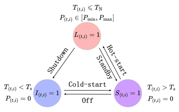
In the coordinated operation of multi-electrolyzer systems, decision-making regarding state transitions and power allocation is governed by variations in the input power, predefined control objectives, and the intrinsic dynamic characteristics of the AWEs. Considering these fluctuating conditions, a state transition model that incorporates the dynamic behavior of the electrolyzers is established, as illustrated in Figure 1 [29,30].

Based on this model, the state variables, input power, and temperature characteristics for the three operational states of a multi-electrolyzer system are defined as follows:

(1)

Shutdown State: At time t, there are $n_{(t)}^{\mathrm{I}}$ electrolyzers in the shutdown state. For the i-th electrolyzer, the shutdown state variable is denoted as $I_{(t,i)}=1$, with an input power of $P_{(t,i)}=0$.

(2)

Standby State: At time t, there are $n_{(t)}^{\mathrm{S}}$ electrolyzers in the standby state. For the i-th electrolyzer, the standby state variable is denoted as $S_{(t,i)}=1$, with an input power of $P_{(t,i)}=0$.

(3)

Production State: At time t, there are $n_{(t)}^{\mathrm{L}}$ electrolyzers operating in a stable hydrogen production state. For the i-th electrolyzer, the production state variable is denoted as $L_{(t,i)}=1$, and its input power $P_{(t,i)}$ is constrained within the allowable operating range $\left[P_{\min },P_{\max }\right]$. The lower bound $P_{\min }$ is strictly maintained to ensure that the hydrogen-in-oxygen concentration remains within safe limits.

Temperature characteristics across different states: When the i-th electrolyzer is in the production state at time t, its operating temperature $T_{(t,i)}$ is maintained at or below the rated temperature $T_{\mathrm{N}}$. If $T_{(t,i)}$ exceeds $T_{\mathrm{N}}$, a heat exchanger activates the cooling water circuit to regulate the temperature back below $T_{\mathrm{N}}$. In the standby state, the temperature $T_{(t,i)}$ remains above the minimum critical temperature $T_{\mathrm{s}}$, which is the lowest temperature required to sustain full-load current under rated voltage limits. In the shutdown state, the temperature drops below this critical threshold ($T_{(t,i)}<T_{\mathrm{s}}$). Since the system lacks auxiliary heating equipment, electrolyzers in both standby and shutdown states rely entirely on natural convection for cooling.

Based on the defined operating states, the state transitions for multiple electrolyzers are categorized into two primary types:

(1)

Cold-Start and Hot-Start Processes (collectively referred to as the startup process): A cold start involves transitioning $n_{(t)}^{\mathrm{I}\_\mathrm{S}}$ electrolyzers from the shutdown state ($I_{(t,i)}=1$) to the standby state ($S_{(t+\tau ,i)}=1$) over a duration of $\tau$. A hot start entails transitioning $n_{(t)}^{\mathrm{S}\_\mathrm{L}}$ electrolyzers from the standby state ($S_{(t,i)}=1$) to the production state ($L_{(t,i)}=1$) over a duration of $\kappa$. These startup processes consume electrical power and typically last for tens of minutes.

(2)

Standby, Off, and Shutdown Processes: These transition processes involve $n_{(t)}^{\mathrm{L}\_\mathrm{S}}$ electrolyzers shifting from the production state to the standby state, $n_{(t)}^{\mathrm{S}\_\mathrm{I}}$ electrolyzers shifting from the standby state to the shutdown state, and $n_{(t)}^{\mathrm{L}\_\mathrm{I}}$ electrolyzers shifting directly from the production state to the shutdown state. During these three specific transition types, the input power drops to zero instantaneously.

Temperature characteristics during state transitions: During the startup process, the electrolyzer generates both hydrogen and heat, leading to an increase in temperature. The cold-start process concludes when the temperature reaches the critical threshold $T_s$, whereas the hot-start process finishes when the temperature reaches the rated value $T_{\mathrm{N}}$. The total duration of the startup process is directly governed by the initial temperature and the input power. Conversely, the durations of the standby, off, and shutdown processes are significantly shorter than the thermal time constant of the electrolyzer; therefore, temperature variations during these specific phases are considered negligible.

Temperature variations are intrinsically linked to the operational states and their transitions. Among these, the startup process—which is highly sensitive to temperature dynamics—serves as the critical factor for the control strategy when formulating state transition plans and allocating power. Consequently, to accurately analyze the startup process, it is essential to establish comprehensive mathematical models encompassing the thermal, electrical, and hydrogen-production dynamics.

2.2. Establishment and Validation of the Thermal, Electrical, and Hydrogen Models

To elucidate the polarization characteristics of the electrolyzer under varying temperatures during the startup process and to determine the trend of temperature variations with respect to input power, it is essential to establish comprehensive electrochemical and thermal models. Concurrently, to quantify the hydrogen production performance of individual electrolyzers scheduled by the control strategy, a hydrogen production rate model is introduced.

(1)

Effect of Temperature Variation on Polarization Characteristics

The electrochemical model characterizes the functional relationship among cell voltage, temperature, and current density under various operational conditions. The overall electrolyzer voltage can be expressed as follows [31]:

$$\left\{\begin{array}{cc}{V}_{(t,i)}\hfill & =N_{\mathrm{cell}}\cdot V_{\mathrm{cell}}(T_{(t,i)},j_{(t,i)})\hfill \\ V_{\mathrm{cell}}\hfill & =V_{\mathrm{rev}}+\left({\mathrm{r}}_1+{\mathrm{r}}_2\cdot T_{(t,i)}\right)\cdot j_{(t,i)}\hfill \\ & +\mathrm{s}\cdot \log \left(\left({\mathrm{t}}_1+{\displaystyle \frac{{\mathrm{t}}_2}{T_{(t,i)}}}+{\displaystyle \frac{{\mathrm{t}}_3}{T_{(t,i)}^2}}\right)\cdot j_{(t,i)}+1\right)\hfill \\ V_{\mathrm{rev}}\hfill & =V_{\mathrm{rev}}^0+{\displaystyle \frac{R{T}_{(t,i)}}{2F}}\ln \left[{\displaystyle \frac{{\left(p-p_{{\mathrm{H}}_2\mathrm{O}}\right)}^{1.5}}{{\alpha }_{{\mathrm{H}}_2\mathrm{O}}}}\right]\hfill \end{array}\right.$$

(1)

where $V_{(t,i)}$ is the voltage of the i-th electrolyzer at time t (V); $N_{\mathrm{cell}}$ is the number of individual cells within the electrolyzer; $V_{\mathrm{cell}}$ is the cell voltage (V); $j_{(t,i)}$ is the current density of the i-th electrolyzer at time i (A·m⁻²); $V_{\mathrm{rev}}$ is the reversible voltage (V); $V_{\mathrm{rev}}^0$ is the standard reversible voltage (V); $\mathrm{R}$ is the universal gas constant (J·mol⁻¹·K⁻¹); $\mathrm{F}$ is the Faraday constant (C·mol⁻¹); $p$ is the operating pressure of the electrolyzer (Pa); $p_{{\mathrm{H}}_2\mathrm{O}}$ is the saturated vapor pressure of water (Pa); ${\alpha }_{{\mathrm{H}}_2\mathrm{O}}$ is the water activity; and ${\mathrm{r}}_1$, ${\mathrm{r}}_2$, $s$, ${\mathrm{t}}_1$, ${\mathrm{t}}_2$ and ${\mathrm{t}}_3$ are empirical coefficients relating to the activation and ohmic overpotentials. The cell voltage calculated by the electrochemical model directly determines the heat generation power, which, together with the heat dissipation power, constitutes the thermal model.

(2)

Dynamic Response of Current Density to Temperature

Based on the law of energy conservation, a lumped-parameter thermal model is adopted to describe the overall temperature dynamics. To avoid the computational intractability of high-dimensional fluid dynamics and ensure the real-time feasibility of the control strategy, the complex spatial temperature gradients within the electrolyzer are neglected. Thus, the rate of temperature change can be derived as follows [31]:

$$\begin{array}{c}{C}_{\mathrm{stack}}{\displaystyle \frac{dT}{dt}}={\dot{Q}}_{\mathrm{gen}}(T_{(t,i)},j_{(t,i)})-{\dot{Q}}_{\mathrm{loss}}(T_{(t,i)})\\ -{\dot{Q}}_{\mathrm{cool}}(T_{(t,i)})-{\dot{Q}}_{\mathrm{exch}}(T_{(t,i)})\\ \left\{\begin{array}{l}{\dot{Q}}_{\mathrm{gen}}=N_{\mathrm{cell}}(V_{\mathrm{cell}}-V_{\mathrm{th}})\cdot j_{(t,i)}\cdot A\\ {\dot{Q}}_{\mathrm{loss}}={\displaystyle \frac{(T_{(t,i)}-T_{\mathrm{a}})}{R_{\mathrm{stack}}}}\\ {\dot{Q}}_{\mathrm{cool}}={\dot{m}}_{\mathrm{lye}}{C}_{\mathrm{lye}}(T_{\mathrm{lye}}-T_{(t,i)})\\ {\dot{Q}}_{\mathrm{exch}}={\dot{m}}_{{\mathrm{H}}_2}{C}_{{\mathrm{H}}_2}(T_{(t,i)}-T_{\mathrm{a}})+{\dot{m}}_{{\mathrm{O}}_2}{C}_{{\mathrm{O}}_2}(T_{(t,i)}-T_{\mathrm{a}})\end{array}\right.\end{array}$$

(2)

where $C_{\mathrm{stack}}$ is the total heat capacity of the electrolyzer (J·K⁻¹); ${\displaystyle \frac{dT}{dt}}$ is the rate of temperature change (K·s⁻¹); ${\dot{Q}}_{\mathrm{gen}}$, ${\dot{Q}}_{\mathrm{loss}}$, ${\dot{Q}}_{\mathrm{cool}}$, and ${\dot{Q}}_{\mathrm{exch}}$ denote the heat generation power from the electrolysis process, the heat dissipation power to the ambient environment, the heat removal power by the cooling water, and the heat dissipation power carried away by gases, respectively (W); $A$ is the cross-sectional area of the electrode (m²); $R_{\mathrm{stack}}$ is the thermal resistance of the electrolyzer (K·W⁻¹); $T_{\mathrm{a}}$ is the ambient temperature (K); ${\dot{m}}_{\mathrm{lye}}$, ${\dot{m}}_{{\mathrm{H}}_2}$, and ${\dot{m}}_{{\mathrm{O}}_2}$ are the mass flow rates of the alkaline solution, hydrogen gas, and oxygen gas, respectively (kg·s⁻¹); and $C_{\mathrm{lye}}$, $C_{{\mathrm{H}}_2}$, and $C_{{\mathrm{O}}_2}$ are the specific heat capacities of the alkaline solution, hydrogen gas, and oxygen gas, respectively (J·kg⁻¹·K⁻¹).

It should be noted that in this system-level framework, the thermal dynamics of auxiliary balance-of-plant components are equivalently aggregated into the cooling heat removal term ${\dot{Q}}_{\mathrm{cool}}$. The rationale for this simplification is based on the control decoupling principle: in actual industrial operations, the thermal equilibrium of these auxiliary components is maintained by local regulatory controllers. Therefore, instead of establishing separate complex differential equations for auxiliary thermal inertia, this aggregated treatment avoids redundant computational burden. It ensures the efficiency of the control strategy while accurately capturing the overall temperature variation trends required for state switching and power allocation.

(3)

Nonlinear Relationship Between Input Power and Hydrogen Production Rate

According to Faraday’s Law, the hydrogen production rate ${\dot{n}}_{(t,i)}$ can be calculated using the following equation:

$${\dot{n}}_{(t,i)}={\displaystyle \frac{N_{\mathrm{cell}}\cdot j_{(t,i)}\cdot A}{2F}}$$

(3)

The hydrogen production rate is directly proportional to the current density, which consequently establishes a temperature-dependent, nonlinear relationship between the hydrogen production rate and the input power $P_{(t,i)}$:

$$\begin{array}{cc}{P}_{(t,i)}& =2\mathrm{F}\cdot {\dot{n}}_{(t,i)}\cdot \left[V_{\mathrm{rev}}+\left({\mathrm{r}}_1+{\mathrm{r}}_2\cdot T_{(t,i)}\right)\cdot {\displaystyle \frac{2\mathrm{F}\cdot {\dot{n}}_{(t,i)}}{N_{\mathrm{cell}}\cdot A}}\right.\\ & \left.+\mathrm{s}\cdot \log \left(\left({\mathrm{t}}_1+{\displaystyle \frac{{\mathrm{t}}_2}{T_{(t,i)}}}+{\displaystyle \frac{{\mathrm{t}}_3}{T_{(t,i)}^2}}\right)\cdot {\displaystyle \frac{2\mathrm{F}\cdot {\dot{n}}_{(t,i)}}{N_{\mathrm{cell}}\cdot A}}+1\right)\right]\end{array}$$

(4)

The equipment specifications and model parameters of the electrolyzer are detailed in

Table 1. Equipment parameters of a 5 MW electrolyzer.

Parameter	Value	Unit
Hydrogen production	1000	Nm3·h−1
DC current	10,200	A
DC voltage	468	V
DC power consumption	≤4.4	kWh·Nm−3
KOH mass fraction	30	%
Operating pressure	2.0	MPa
Operating temperature	90 ± 5	°C

and

Table 2. Model parameters of the 5 MW electrolyzer.

Parameter	Value	Unit
$\mathrm{Number}\mathrm{of}\mathrm{cells}(N_{\mathrm{cell}}$)	234	units
Universal gas constant ($\mathrm{R}$)	8.314	J·mol−1·K−1
Faraday constant ($\mathrm{F}$)	96,485	C·mol−1
Electrode Area ($A$)	2.91	m2
$\mathrm{Specific}\mathrm{Heat}\mathrm{Capacity}\mathrm{of}\mathrm{Hydrogen}(C_{{\mathrm{H}}_2}$)	14,300	J·kg−1·K−1
$\mathrm{Specific}\mathrm{Heat}\mathrm{Capacity}\mathrm{of}\mathrm{Oxygen}(C_{{\mathrm{O}}_2}$)	919	J·kg−1·K−1
$\mathrm{Ambient}\mathrm{Temperature}(T_{\mathrm{a}}$)	298.15	K

, respectively:

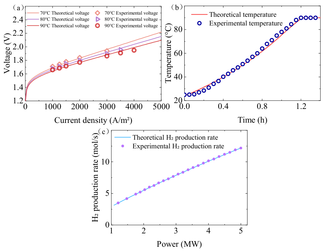
Separate experiments were conducted to compare the simulated model data with the actual operational data of a 5 MW electrolyzer(Tianjin Mainland Hydrogen Equipment Co., Ltd., Tianjin, China) as shown in Figure 2:

• Electrochemical Model Validation: The electrolyzer was operated at three constant temperatures (70 °C, 80 °C, and 90 °C). Under each thermal condition, different current densities were applied, and the corresponding cell voltages were measured.
• Thermal Model Validation: The electrolyzer was started from an ambient temperature of 25 °C in a constant-voltage mode at the rated voltage, and the temperature variations over time were recorded.
• Hydrogen Production Rate Model Validation: The electrolyzer temperature was maintained at a constant 90 °C. Various input powers were applied, and the corresponding hydrogen production rates were measured.

Temperature variations within the electrolyzer alter its polarization characteristics, ensuring that a specific input power under the control strategy corresponds to a deterministic set of current and voltage values. Specifically, the current is directly correlated with the hydrogen production rate ${\dot{n}}_{(t,i)}$, while the current and voltage synergistically dictate the rate of temperature change, thereby forming a tight thermo-electro-hydrogen coupling relationship. Based on this coupled model, a quantitative analysis of the startup process for a multi-electrolyzer hydrogen production system is conducted.

2.3. Temperature–Power Adaptive Relationship During Startup

Alkaline electrolyzers typically employ two primary startup modes: constant-voltage startup and step-current startup. The trajectory of current density loading during the startup process is deterministic and follows specific rules. At any given time t during the startup phase, the maximum allowable loading current density is constrained by the rated voltage to ensure safety and gas purity. This constraint is mathematically determined by Equation (5):

$$j_{(t,i)}^{\max }=\min \left(j_{\mathrm{N}},\sup \left\{\left.j_{(t,i)}\right|V_{(t,i)}\le V_{\mathrm{N}}\right\}\right)$$

(5)

where $j_{(t,i)}^{\max }$ represents the maximum allowable current density of the i-th electrolyzer at time t (A·cm⁻²); $j_{\mathrm{N}}$ is the rated current density (A·cm⁻²); and $V_{\mathrm{N}}$ is the rated voltage of the electrolyzer (V). The maximum current density is defined as the lesser of the rated current density and the highest current density permissible without exceeding the rated voltage limit.

Consequently, the feasible range for the current density at the subsequent time step t + 1 is derived as follows:

$$j_{(t+1,i)}\in \left[j_{(t,i)},\min (j_{(t,i)}+u{j}_{\mathrm{N}},j_{(t+1,i)}^{\max })\right]$$

(6)

where $u$ denotes the maximum current density ramp rate coefficient. The lower bound of this interval is determined by the current density at the previous time step $j_{(t,i)}$, while the upper bound is constrained by the minimum of two values: the limit imposed by the ramp rate constraint ($j_{(t,i)}+u{j}_{\mathrm{N}}$) and the maximum allowable current density $j_{(t+1,i)}^{\max }$ calculated from Equation (5).

Once the current density at time t is determined based on the specific startup mode, the rate of temperature change at time t is calculated via the thermal model (Equation (2)) to update the temperature for the next time step t + 1:

$$T_{(t+1,i)}=\min (T_{(t,i)}+{\displaystyle \frac{dT}{dt}}(T_{(t,i)},j_{(t,i)})\cdot \Delta t,T_{\mathrm{N}})$$

(7)

Subject to the rated temperature constraint, the temperature at time t + 1 is obtained by integrating the rate of temperature change, which is determined by the current density and temperature at time t.

Power, serving as the core dispatch variable in the control strategy, can be calculated based on the determined current density and the corresponding cell voltage:

$$P_{(t,i)}=j_{(t,i)}\cdot A\cdot V_{(t,i)}(j_{(t,i)},T_{(t,i)})$$

(8)

Using the critical temperature $T_{\mathrm{s}}$ and the rated temperature $T_{\mathrm{N}}$ as the judgment criteria, the duration of the cold-start process $\tau$ (transitioning from the shutdown state $I_{(t,i)}=1$ to the standby state $S_{(t+\tau ,i)}=1$) and the hot-start process $\kappa$ (transitioning from the standby state $S_{(t,i)}=1$ to the production state $L_{(t+\kappa ,i)}=1$) can be calculated as follows:

$$\left\{\begin{array}{l}\tau ={\displaystyle {\int }_{T_{0(t,i)}}^{T_{\mathrm{s}}}\frac{1}{\frac{dT}{dt}(T_{(t,i)},j_{(t,i)})}dT}\\ \kappa ={\displaystyle {\int }_{T_s}^{T_{\mathrm{N}}}\frac{1}{\frac{dT}{dt}(T_{(t,i)},j_{(t,i)})}dT}\end{array}\right.$$

(9)

where $T_{0(t,i)}$ is the initial temperature of the i-th electrolyzer starting at time t (K).

The dynamic response of the startup process operates on a timescale of seconds, whereas the dispatch period of the control strategy is typically in minutes. To bridge this temporal discrepancy and integrate the startup dynamics into the scheduling framework, the startup power and its per-unit value are utilized to characterize the overall dynamic features of the startup process:

$$\left\{\begin{array}{l}{P}_{(t,i)}^{\mathrm{st}}={\displaystyle \frac{1}{{\tau }_{(t,i)}+{\kappa }_{(t,i)}}}{\displaystyle {\int }_0^{{\tau }_{(t,i)}+{\kappa }_{(t,i)}}{P}_{(s,i)}ds}\\ P_{(t,i)}^{\mathrm{st}\ast }={\displaystyle \frac{P_{(t,i)}^{\mathrm{st}}}{P_{\max }}}\end{array}\right.$$

(10)

where $P_{(t,i)}^{\mathrm{st}}$ represents the equivalent startup power of the i-th electrolyzer initiating startup at time t, and $P_{(t,i)}^{\mathrm{st}\ast }$ denotes the per-unit (normalized) value of this startup power relative to the maximum operating power $P_{\max }$.

The total hydrogen production during the entire startup process is obtained by integrating the hydrogen production rate over time:

$$Q_{(t,i)}^{\mathrm{st}}={\displaystyle {\int }_0^{{\tau }_{(t,i)}+{\kappa }_{(t,i)}}{\dot{n}}_{(s,i)}}ds$$

(11)

where $Q_{(t,i)}^{\mathrm{st}}$ represents the cumulative hydrogen production (mol) of the i-th electrolyzer throughout the entire startup process initiated at time t.

To analyze the dynamic characteristics of the startup process quantitatively, the following simulation conditions were established:

• Electrolyzer Rated Operating Point: Current 10,200 A, Voltage 468 V, Temperature 90 °C.
• Initial Conditions: The startup process commences at an initial temperature of 25 °C.
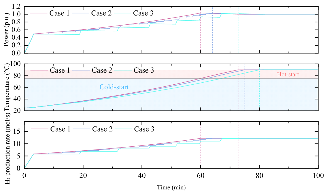
• Startup Methods: Three distinct startup modes were evaluated: (1) Constant-voltage startup (Case 1); (2) Step-current startup with a step size of 580 A (Case 2); and (3) Step-current startup with a step size of 880 A (Case 3).

Under identical initial temperatures, the dynamic responses of power, temperature, and hydrogen production rate for these three startup methods are compared in Figure 3.

A comparative analysis of the startup characteristics reveals distinct trade-offs. The constant-voltage startup mode achieves the shortest duration, with cold- and hot-start times of 60.13 min and 12.80 min, respectively. However, this speed comes at the cost of the highest power demand, with a per-unit startup power of 0.7516, and yields the lowest total hydrogen production of 873.46 Nm³.

Conversely, for the step-current startup modes with step sizes of 580 A and 880 A, the per-unit startup power requirements are significantly reduced to 0.7354 and 0.7033, respectively. This demonstrates that the electrolyzer can be successfully started at lower input power levels. However, this reduction in power demand necessitates an extension in startup duration: the cold-start times increase to 62.32 min and 67.25 min, and the hot-start times to 12.77 min and 12.85 min, respectively. Notably, the total hydrogen production increases to 884.40 Nm³ and 908.24 Nm³, respectively. This confirms that for a known initial temperature, there exists a unique, deterministic relationship between the chosen startup method (and thus the startup power trajectory) and the startup duration.

Taking the constant-voltage startup as an illustrative example: when the electrolyzer reaches the rated current density, the temperature point $T_{(t,i)}=T_{\mathrm{s}}=75.32$ °C serves as the boundary dividing the process into cold-start and hot-start phases. Throughout the startup, the temperature exhibits a monotonic increase until it reaches the rated temperature $T_{\mathrm{N}}$. Interestingly, the rate of temperature rise first increases and then decreases, reaching its peak value at $T_{(t,i)}=T_{\mathrm{s}}$.

• Cold-Start Phase ($T_{(t,i)}\le T_{\mathrm{s}}$): The electrolyzer voltage is stabilized at the rated voltage constraint. Consequently, the current density and power must adhere to the temperature-dependent upper limit to prevent voltage overshoot, which could compromise hydrogen purity. As the temperature rises, this allowable current limit increases, leading to higher heat generation power. Therefore, the rate of temperature rise exhibits an accelerating trend during this phase.
• Hot-Start Phase ($T_{(t,i)}>T_{\mathrm{s}}$): The current density remains constant at the rated value. As the temperature continues to rise, the cell voltage decreases due to improved electrochemical kinetics. This reduction in voltage leads to a decrease in input power and heat generation. Consequently, the rate of temperature rise gradually decelerates as the temperature approaches $T_{\mathrm{N}}$, until the startup process concludes.

Under identical initial temperature conditions, utilizing different startup methods significantly alters both the startup power and the transition duration. However, in actual operations characterized by fluctuating renewable energy inputs, the control strategy dictates the electrolyzer startup timing dynamically based on real-time system power availability. Consequently, the initial temperature of an electrolyzer dynamically varies rather than remaining fixed at the ambient temperature. To further analyze the specific impact of varying initial temperatures on startup characteristics, the following simulation conditions were established:

• Electrolyzer Rated Operating Point: Current 10,200 A, Voltage 468 V, Temperature 90 °C.
• Initial Startup Temperatures: 25 °C, 50 °C, and 75 °C.
• Startup Method: Constant-voltage startup.

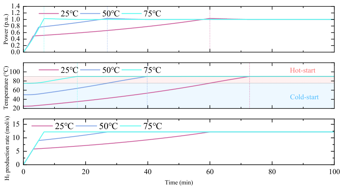
Employing the same constant-voltage startup method, the dynamic responses of power, temperature, and hydrogen production rate across the three distinct initial temperatures are compared, as illustrated in Figure 4.

Based on Figure 4, the specific startup parameters under different initial temperatures are summarized in

Table 3. Startup parameters at different initial temperatures.

Initial Temperature (°C)	Startup Power (p.u.)	Cold-Start Time (min)	Hot-Start Time (min)	Hydrogen Production (Nm3)
25	0.7516	60.0	13.0	873.46
50	0.8634	27.1	12.8	551.79
75	0.8053	3.3	14.1	230.21

:

As the initial temperature rises, the cold-start time is significantly curtailed. Conversely, the hot-start time exhibits a non-monotonic trend, initially decreasing and subsequently increasing. Notably, at an initial temperature of 75 °C, the hot-start time paradoxically increases rather than decreases. This phenomenon occurs because, during the very beginning of the startup phase, the current density must rise linearly from zero due to the strict ramp rate constraints. At this moment, the heat generation power is relatively low, resulting in a sluggish temperature rise. Since 75 °C is already in close proximity to the critical temperature threshold $T_{\mathrm{s}}$, the majority of this constrained, slow-ramping linear current density loading phase is inadvertently incorporated into the hot-start phase, thereby prolonging the overall hot-start duration.

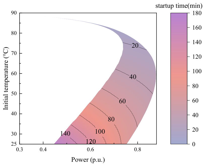
The preceding analysis independently reveals the isolated effects of the chosen startup method and the initial temperature on the dynamic startup characteristics. To enable the control strategy to meticulously plan state transitions and allocate power, it is imperative to comprehensively consider the strongly coupled effects of both factors on startup power and startup duration. Therefore, by continuously sweeping the initial temperature from the ambient state (25 °C) to the rated operational state (90 °C), a comprehensive temperature–power adaptive relationship is formulated, utilizing the initial temperature and startup power as independent variables, and the overall startup time as the response variable.

Figure 5 illustrates the constrained feasible region of startup power at any given initial temperature, alongside the deterministic startup time corresponding to each specific power value within this envelope. This contour mapping provides a rigorous decision-making foundation for state switching and power allocation within the control strategy. The theoretical boundaries—namely the maximum and minimum startup powers and their corresponding extreme values of startup time—under representative initial temperatures are detailed in

Table 4. Boundaries of startup power and extreme values of startup time at different initial temperatures.

Initial Temperature (°C)	Minimum Startup Power (p.u.)	Maximum Startup Power (p.u.)	Maximum Startup Time (min)	Minimum Startup Time (min)
30	0.4832	0.7796	137.97	64.98
50	0.6279	0.8634	57.27	39.85
70	0.7335	0.8475	22.20	21.33

:

• Minimum Startup Power: This boundary is defined by the startup method utilizing the maximum allowable step current. Operating under this mode, the initial current density increases linearly while strictly adhering to ramping constraints, forcing the voltage to rise concurrently. Upon reaching the rated voltage limit, the current density is maintained constant until the startup concludes. While this method minimizes the startup power, it incurs the absolute maximum startup time. The trajectory of this minimum startup power lower limit as a function of the initial temperature is governed by two competing factors: (1) The polarization characteristics of the electrolyzer: under the rated voltage constraint, a higher initial temperature yields a higher steady-state current density, which consequently increases the minimum startup power. (2) The proportion of the linear loading phase: as the initial temperature approaches the rated temperature, the linear loading phase occupies a larger proportion of the total startup duration, which pulls the equivalent minimum startup power downwards.
• Maximum Startup Power: This boundary is strictly bounded by the constant-voltage startup mode, achieving the absolute minimum startup time.

Based on the quantitative relationships established above, the total startup time can be mathematically expressed as a bivariate function of the initial temperature and the startup power:

$$\tau +\kappa =f_{\mathrm{st}}(P_{(t,i)}^{\mathrm{st}},T_{0(t,i)})$$

(12)

where $\tau +\kappa$ represents the total startup time; $f_{\mathrm{st}}$ is the nonlinear function characterizing the temperature–power adaptive relationship depicted in Figure 5; $P_{(t,i)}^{\mathrm{st}}$ is the startup power; and $T_{0(t,i)}$ is the initial temperature.

The initial temperature precisely dictates the viable interval for startup power. Subsequently, this temperature, acting synergistically with a selected startup power within that interval, deterministically dictates the required startup duration. During the real-time execution of the control strategy, the initial temperature parameter is directly acquired from the electrolyzer’s physical temperature sensors.

In conclusion, the mathematical modeling in this section successfully uncovers the quantitative coupling among startup time, initial temperature, and startup power. This inherent relationship is a pivotal constraint that must be incorporated into state transitions and power allocation. Building upon this, an optimized scheduling framework fully integrating this temperature–power adaptive relationship is developed in the subsequent section to achieve coordinated multi-electrolyzer control under highly fluctuating operating conditions.

2.4. Temperature–Power Adaptive Multi-Electrolyzer Control Optimization Strategy

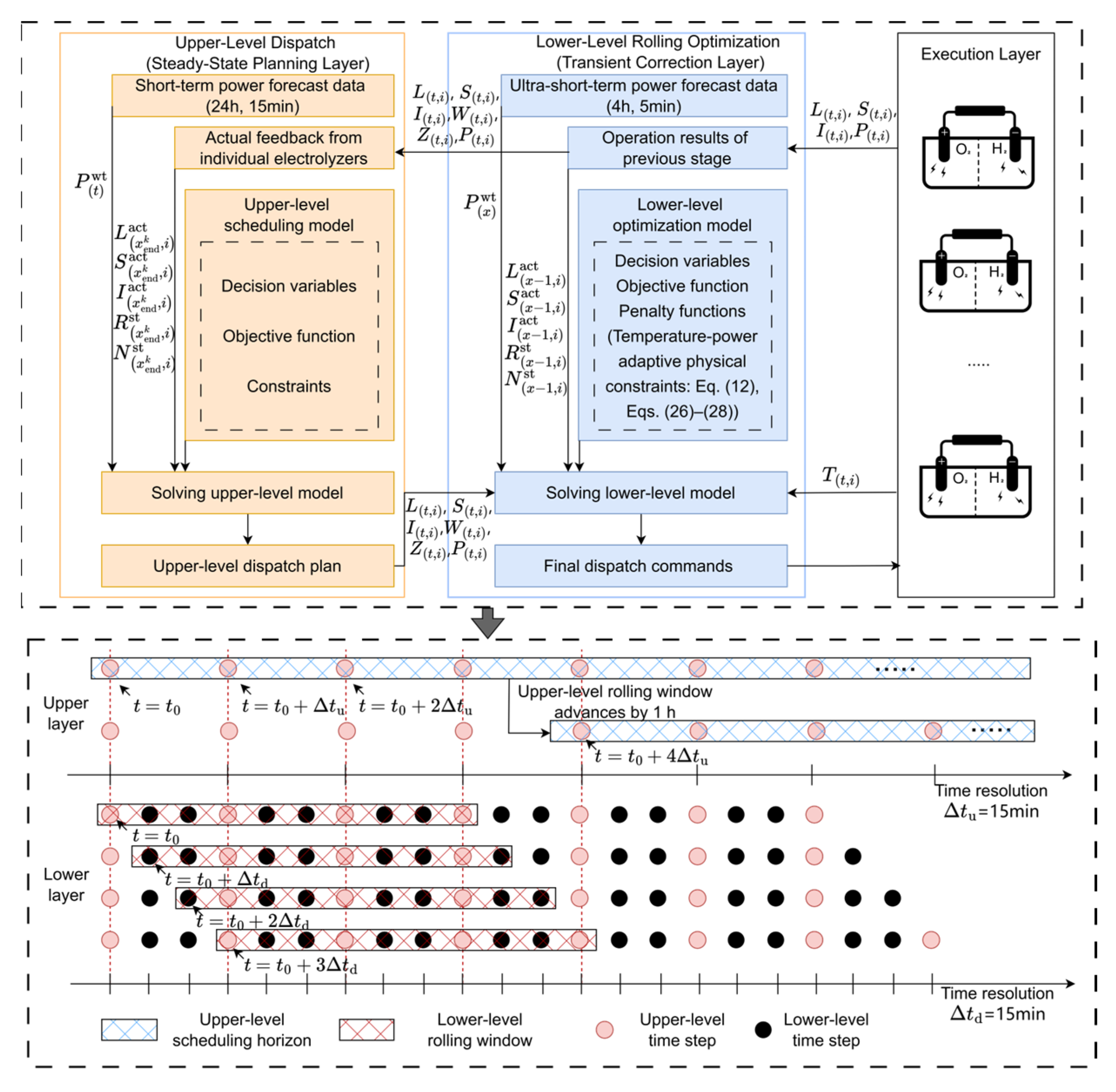
Under fluctuating renewable energy inputs, the dynamic operational characteristics of electrolyzers, particularly during the startup process, are significantly altered by temperature variations. To enable the control strategy to account for these impacts during dispatch, a temperature–power adaptive dual-layer optimization scheduling framework is adopted, as illustrated in Figure 6.

This dual-layer framework is designed to satisfy distinct computational demands. The upper layer employs a MILP model, which effectively handles the large-scale optimization problem involving coupled binary operational state variables and continuous power allocation variables inherent in multi-electrolyzer dispatch. Thus, MILP provides a rigorous foundation for formulating global state-switching baselines based on short-term forecasts. However, to guarantee computational tractability, the upper-level MILP inevitably relies on linearized assumptions. To handle the nonlinearities introduced to ensure the effectiveness of the control strategy, the lower layer adopts MOA. Driven by real-time temperature feedback ($T_{(t,i)}$), the lower layer utilizes MOA to directly embed the nonlinear temperature–power adaptive relationships and the accurate hydrogen production curves into the model. Consequently, this dual-layer architecture enables the control strategy to solve the multi-unit commitment problem while considering the impacts of actual temperature variations.

2.4.1. Upper-Level Mixed-Integer Linear Programming Scheduling Model

The MILP model aims to maximize total hydrogen production. It operates on 24 h short-term renewable energy forecast data with a 15 min time resolution and is solved using the CPLEX solver (Version 12.10.0.0, IBM, Armonk, NY, USA). To enhance system robustness, the upper scheduling layer receives the multi-electrolyzer states and power data from the lower rolling optimization layer every 4 h, and subsequently updates the scheduling plan for the remaining time horizon. The mathematical formulation of this MILP model comprises three core components: decision variables, the objective function, and constraints.

Decision Variables: The production ($L_{(t,i)}$), standby ($S_{(t,i)}$), and shutdown ($I_{(t,i)}$) states, along with the cold-start ($Y_{(t,i)}$), hot-start ($W_{(t,i)}$), and standby, off, shutdown transition ($Z_{(t,i)}$) actions, are defined as binary decision variables. The input power ($P_{(t,i)}$) is defined as a continuous decision variable.

Objective Function: The upper-level model is designed to maximize the total hydrogen production. To ensure the solvability of the MILP problem, the hydrogen production rate is approximated as a linear function of the input power, expressed as follows:

$${{\dot{n}}^{\prime }}_{(t,i)}=a\cdot P_{(t,i)}+b$$

(13)

where ${{\dot{n}}^{\prime }}_{(t,i)}$ is the hydrogen production rate of the i-th electrolyzer at time t calculated via the linear model (mol/s); $a$ and $b$ are the slope and intercept parameters of this linear function, respectively. It should be noted that the upper-layer model is primarily responsible for determining discrete state transitions rather than precise real-time power allocation. Therefore, this linear approximation guarantees the global solvability of the MILP model while introducing minimal deviations that do not compromise the accuracy of macroscopic state-switching decisions [19]. The objective function of the MILP problem can be expressed as:

$$Q^{\prime }={\displaystyle \sum _{t=1}^T{\displaystyle \sum _{i=1}^N{{\dot{n}}^{\prime }}_{(t,i)}}}\Delta t_{\mathrm{u}}$$

(14)

where $Q^{\prime }$ is the total hydrogen production calculated using the linear hydrogen production rate model over the production cycle (mol); T is the number of time steps in the production cycle; N is the total number of electrolyzers in the hydrogen production system; and $\Delta t_{\mathrm{u}}$ is the time interval of one upper-level time step (s).

Constraints: The constraints that the system must satisfy include power balance constraints, input power constraints, and electrolyzer state constraints.

(1)

Power Balance Constraint

The total input power of multiple electrolyzers must not exceed the available power generation from renewable energy sources at any given time.

$$0\le \sum _{i=1}^N{P}_{(t,i)}\le P_{(t)}^{\mathrm{wt}},\forall t\in T$$

(15)

where $P_{(t)}^{\mathrm{wt}}$ is the available power output of renewable energy at time t (MW).

(2)

Input Power Constraints

When an electrolyzer is in the production state, its input power limits are as follows:

$$\begin{array}{c}{P}_{\min }{L}_{(t,i)}\le P_{(t,i)}\le P_{\max }{L}_{(t,i)}\\ \forall t\in T,\forall i\in N\end{array}$$

(16)

where $P_{\min }$ and $P_{\max }$ represent the minimum and maximum input power of the electrolyzer in the production state, respectively (MW). Simultaneously, power variations must satisfy the ramp rate limits, constrained as follows:

$$\begin{array}{c}\left\{\begin{array}{l}{P}_{(t,i)}-P_{(t-1,i)}\le \mathsf{\Delta }{P}^{\mathrm{RU}}\\ P_{(t-1,i)}-P_{(t,i)}\le \mathsf{\Delta }{P}^{\mathrm{RD}}+\left(1-L_{(t,i)}\right)P_{\max }\end{array}\right.\\ \forall t\in T,\forall i\in N\end{array}$$

(17)

where $\mathsf{\Delta }{P}^{\mathrm{RU}}$ and $\mathsf{\Delta }{P}^{\mathrm{RD}}$ are the maximum ramp-up and ramp-down rate limits of the electrolyzer power, respectively (MW).

To ensure the solvability of the upper-layer model, the startup powers for cold start and hot start are set to fixed power reference values, as formulated in Equation (18):

$$\begin{array}{c}\left\{\begin{array}{l}{P}_{(t,i)}\ge P_{\mathrm{cs}}-M\cdot (1-Y_{(t,i)})\\ P_{(t,i)}\le P_{\mathrm{cs}}+M\cdot (1-Y_{(t,i)})\end{array}\right.\\ \left\{\begin{array}{l}{P}_{(t,i)}\ge P_{\mathrm{hs}}-M\cdot (1-W_{(t,i)})\\ P_{(t,i)}\le P_{\mathrm{hs}}+M\cdot (1-W_{(t,i)})\end{array}\right.\\ \forall t\in T,\forall i\in N\end{array}$$

(18)

where $P_{\mathrm{cs}}$ and $P_{\mathrm{hs}}$ are the reference powers for the cold start and hot start of the electrolyzer, respectively (MW), and M is a sufficiently large positive constant utilized to relax the constraints when the binary variables are zero.

(3)

Electrolyzer State Constraints

Each electrolyzer can only be in one state at any arbitrary time t.

$$S_{(t,i)}+L_{(t,i)}+I_{(t,i)}=1,\forall t\in T,\forall i\in N$$

(19)

In the upper-level model, during the startup process where the electrolyzer transitions from the shutdown state to the production state, the cold-start process must be maintained for $e$ consecutive time steps, and the hot-start process must be maintained for $f$ consecutive time steps.

$$\begin{array}{c}\left\{\begin{array}{l}{Y}_{(t,i)}\ge I_{(t-1,i)}+S_{(t,i)}-1\\ {\displaystyle \sum _{k=0}^{e-1}}{S}_{(t+k,i)}\ge {\displaystyle \sum _{k=0}^{e-1}}{Y}_{(t,i)}\end{array}\right.\\ \forall t\in T-e+1,\forall i\in N\end{array}$$

(20)

$$\begin{array}{c}\left\{\begin{array}{l}{W}_{(t,i)}\ge S_{(t-1,i)}+L_{(t,i)}-1\\ {\displaystyle \sum _{k=0}^{f-1}}{S}_{(t+k,i)}\ge {\displaystyle \sum _{k=0}^{f-1}}{W}_{(t,i)}\end{array}\right.\\ \forall t\in T-f+1,\forall i\in N\end{array}$$

(21)

To prevent rapid degradation of system lifespan caused by extreme load imbalances, constraints on the balancing of start–stop cycles and operating time for each electrolyzer are introduced.

$$\begin{array}{l}\left\{\begin{array}{c}{N}_{(T,i)}^{\mathrm{st}}={\displaystyle \sum _{\mathrm{t}=1}^T{W}_{(t,i)}}\\ R_{(T,i)}^{\mathrm{st}}={\displaystyle \sum _{\mathrm{t}=1}^T{L}_{(t,i)}}\end{array}\right.\\ \left\{\begin{array}{c}\left|N_{(T,i)}^{\mathrm{st}}-N_{(T,j)}^{\mathrm{st}}\right|\le \Delta N_{\max }^{\mathrm{st}}\\ \left|R_{(T,i)}^{\mathrm{st}}-R_{(T,j)}^{\mathrm{st}}\right|\le \Delta R_{\max }^{\mathrm{st}}\end{array}\right.\\ \forall i,j\in N,i\ne j\end{array}$$

(22)

where $N_{(T,i)}^{\mathrm{st}}$ is the number of start–stop cycles for the i-th electrolyzer during the production cycle; $\Delta N_{\max }^{\mathrm{st}}$ is the maximum allowable difference in start–stop cycles among different electrolyzers; $R_{(T,i)}^{\mathrm{st}}$ is the operating time for the i-th electrolyzer during the production cycle; and $\Delta R_{\max }^{\mathrm{st}}$ is the maximum allowable difference in operating time among different electrolyzers. Considering the startup and shutdown events triggered by input power fluctuations, a minimum operational time constraint is introduced to limit frequent state transitions of electrolyzers within a short timeframe.

$$\begin{array}{c}\left\{\begin{array}{l}{\displaystyle \sum _{k=0}^{\min (t_{\mathrm{on}}-1,T-t)}}{L}_{(t+k,i)}\ge t_{\mathrm{on}}\cdot (L_{(t,i)}-L_{(t-1,i)})\\ {\displaystyle \sum _{k=0}^{\min (t_{\mathrm{off}}-1,T-t)}}{I}_{(t+k,i)}\ge t_{\mathrm{off}}\cdot (I_{(t,i)}-I_{(t-1,i)})\end{array}\right.\\ \forall t\in \left[2,\dots ,T\right],\forall i\in N\end{array}$$

(23)

where $t_{\mathrm{on}}$ and $t_{\mathrm{off}}$ are the minimum continuous production time steps and minimum downtime steps of the electrolyzer, respectively.

2.4.2. Lower-Level Rolling Optimization Model Based on MOA

Within the framework of the upper-level scheduling plan, the lower-level rolling optimization layer executes high-resolution real-time power allocation. Based on a 4 h ultra-short-term renewable energy power forecast, it operates with an optimization window of 15 min and a rolling step of 5 min. By integrating the quantitative temperature–power adaptive relationship and acquiring the real-time status, temperature, and power data of each electrolyzer, the Mongoose Optimization Algorithm (MOA) is applied to optimize the power distribution. This process effectively corrects the deviations introduced by the linearization approximations and fixed parameters in the upper-level MILP model.

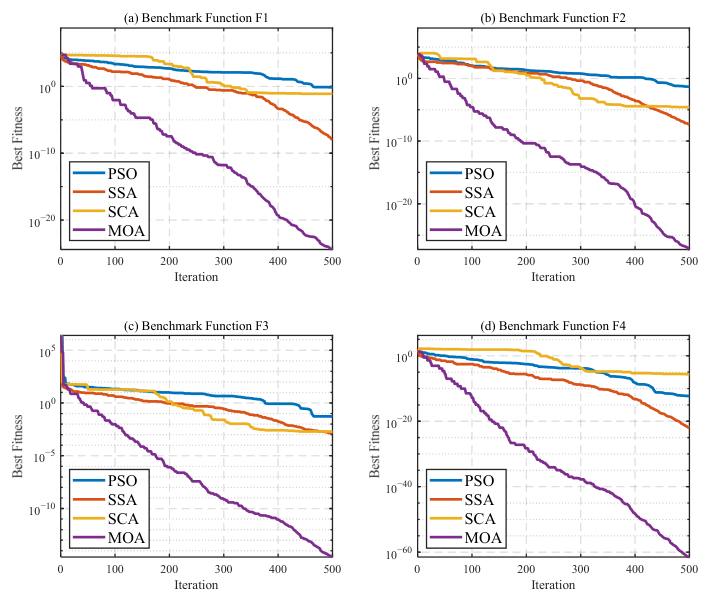
Compared to the upper-level scheduling model, the lower-level rolling optimization aims to achieve more precise real-time control by deeply fusing the temperature–power adaptive relationship. The primary improvements are twofold: first, it dynamically optimizes the startup power based on the real-time temperature of the electrolyzers and the temperature–power adaptive constraints; second, it employs a more accurate, nonlinear hydrogen production rate model to dynamically calibrate the upper-level power allocation scheme. To efficiently and accurately solve the lower-layer problem of the group control strategy, this paper employs an enhanced MOA. Compared to classic metaheuristic algorithms such as Particle Swarm Optimization, the enhanced algorithm exhibits significantly higher precision, a faster convergence rate that effectively reduces computational cost, and stronger scalability. Crucially, this lower-level optimization exhibits exceptional real-time applicability, requiring an average execution time of approximately 2.2 s per rolling cycle, which fully satisfies the 5 min online dispatch requirement. A detailed baseline performance validation, along with rigorous proofs of computational complexity and hardware scalability, are provided in Appendix A.

The state and state-transition variables from the upper-level plan must be accurately mapped to the lower layer. Let $x_0$ denote the starting time step of the lower-level rolling window. This window encompasses three consecutive lower-level time steps $x=x_0,x_0+1,x_0+2$, which correspond to a single upper-level scheduling time step $t=⌈x_0/3⌉$. Within the lower-level window, the state variables of each electrolyzer remain consistent with the upper-level plan. The cold-start transition action is strictly mapped to the first time step ($x_0$) of the lower-level window:

$$Y_{(x,i)}=\left\{\begin{array}{cc}{Y}_{(t,i)},& x\in \left\{x_0\right\}\\ 0,& x\in \left\{x_0+1,x_0+2\right\}\end{array}\right.$$

(24)

where $x_0$ is the cold-start indicator variable for the i-th electrolyzer at the lower-level time step x.

The decision variable for the lower-level rolling optimization is the power matrix of all electrolyzers within the current window, which constitutes the optimization individual (solution vector) in the MOA:

$$\mathit{P}=\left[\begin{array}{cccc}{P}_{(x_0,1)}& P_{(x_0,2)}& \dots & P_{(x_0,N)}\\ P_{(x_0+1,1)}& P_{(x_0+1,2)}& \dots & P_{(x_0+1,N)}\\ P_{(x_0+2,1)}& P_{(x_0+2,2)}& \dots & P_{(x_0+2,N)}\end{array}\right]$$

(25)

For electrolyzers that are not undergoing a startup process, their upper and lower power limits, as well as ramp rate constraints, are identical to those in the upper-level model, as defined in Equations (16) and (17). For electrolyzers currently in the startup process, an auxiliary variable—the remaining startup time steps $R_{(x,i)}$—is introduced:

$$\left\{\begin{array}{cc}\hfill R_{(x,i)}& =Y_{(x,i)}\cdot ⌈{\displaystyle \frac{\tau (P_{(x,i)}^{\mathrm{st}},T_{0(x,i)})+\kappa (P_{(x,i)}^{\mathrm{st}},T_{0(x,i)})}{\Delta t_{\mathrm{d}}}}⌉\hfill \\ \hfill R_{(x+1,i)}& =\max \left(0,R_{(x,i)}-1\right)\hfill \end{array}\right.$$

(26)

where $R_{(x,i)}$ is the number of remaining startup time steps for the i-th electrolyzer at the lower-level time step x; $P_{(x,i)}^{\mathrm{st}}$ is the startup power of the i-th electrolyzer initiating startup at time step x (MW); $T_{0(x,i)}$ is the initial temperature of the i-th electrolyzer initiating startup at time step x (K); and $\Delta t_{\mathrm{d}}$ is the time resolution of the lower layer (s). The variable $R_{(x,i)}$ is obtained by discretizing the total startup time and is strictly decremented by one after each passing time step.

To guarantee that the optimized startup power falls within the feasible power boundaries dictated by the current initial temperature, this hard constraint is transformed into a penalty function:

$${\psi }_{\mathrm{st}}\left(P_{(x,i)}^{\mathrm{st}},T_{0(x,i)}\right)={\left[\max \left(0,P_{\min }^{\mathrm{st}}\left(T_{0(x,i)}\right)-P_{(x,i)}^{\mathrm{st}}\right)\right]}^2+{\left[\max \left(0,P_{(x,i)}^{\mathrm{st}}-P_{\max }^{\mathrm{st}}\left(T_{0(x,i)}\right)\right)\right]}^2$$

(27)

where ${\psi }_{\mathrm{st}}$ is the penalty function for startup power limit violations. Furthermore, during the uncompleted startup time steps, the input power of the electrolyzer is rigidly constrained to equal its designated startup power using another penalty function:

$${\psi }_{\mathrm{eq}}\left(\mathit{P}\right)={\displaystyle \sum _{x=x_0}^{x_0+2}{\displaystyle \sum _{i=1}^N\mathbb{I}\left\{R_{(x,i)}>0\right\}}}\cdot {\left(P_{(x,i)}-P_{(x,i)}^{\mathrm{st}}\right)}^2$$

(28)

where ${\psi }_{\mathrm{eq}}$ is the penalty function for the input power deviation during the startup process, and $\mathbb{I}\left\{·\right\}$ represents the indicator function, which equals 1 if the condition is true and 0 otherwise.

The objective function of the lower-level MOA is formulated to maximize the total hydrogen production of the system within the rolling window:

$$Q={\displaystyle \sum _{x=x_0}^{x_0+2}{\displaystyle \sum _{i=1}^N\left[1-\min \left(1,R_{(x,i)}\right)\right]\cdot {\dot{n}}_{(x,i)}\cdot \Delta t_{\mathrm{d}}}}+\left[\min \left(1,R_{(x,i)}\right)\right]\cdot Q_{(x,i)}^{\mathrm{st}}$$

(29)

where $Q$ is the total hydrogen production within the rolling window (mol). The first term in Equation (29) represents the hydrogen produced by electrolyzers that have fully completed the startup process at time step x, while the second term accounts for the accumulated hydrogen produced by electrolyzers still undergoing the startup process. Specifically, the hydrogen production rate ${\dot{n}}_{(x,i)}$ in Equation (29) employs the temperature-dependent nonlinear physical model detailed in Equations (3) and (4). By replacing the linear approximation ${{\dot{n}}^{\prime }}_{(t,i)}$ used in the upper layer to correct potential physical deviations, this formulation ensures the actual effectiveness of the control strategy.

By deeply integrating the temperature–power adaptive relationship, this dual-layer optimization scheduling framework establishes a highly robust control strategy, effectively adapting to the profound impacts of fluctuating input power and thermal dynamics on operational characteristics.

3. Results and Discussion

3.1. Simulation Setup and Comparative Strategies Under Fluctuating Scenarios

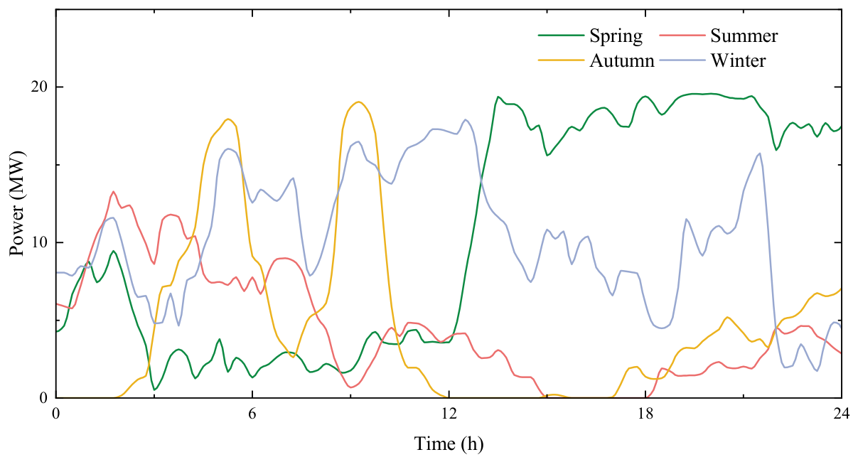
To verify the effectiveness of the proposed control strategy, a simulation case study was conducted using typical seasonal daily wind power data from a wind farm with a rated installed capacity of 20 MW, as illustrated in Figure 7. Specifically, it is important to note that the total input power supplied to the multi-electrolyzer hydrogen production system represents the wind power output after regulation by the Energy Storage System (ESS).

A comparative analysis was conducted among four strategies: (1) the Daisy Chain Control Strategy, (2) the Equal Allocation Control Strategy, (3) the Rotation Control Strategy, and (4) the proposed Multi-Electrolyzer Control Optimization Strategy based on Temperature–Power Adaptation. To ensure a rigorous comparison, the Daisy Chain, Equal Allocation, and Rotation strategies employed fixed baseline startup times and startup powers (with the Rotation strategy additionally employing a fixed 4 h priority shift schedule). These strategies neglect the dynamic operational characteristics affected by the temperature variations of the electrolyzers under fluctuating conditions, particularly during the startup process, where temperature changes are the most rapid and substantial. Meanwhile, all other initial conditions, system configurations, and constraint sets remained consistent with those of the proposed adaptive strategy.

The specific initialization parameters for the simulation are detailed in

Table 5. Initial conditions for the control strategy.

Parameter	Value	Unit
Rated power of electrolyzer	5	MW
Number of electrolyzers	3	units
Initial power of electrolyzer	0	MW
Initial temperature of electrolyzer	25	°C
Number of shutdown units	3	units
Upper-layer time resolution	15	min
Lower-layer time resolution	5	min

, and the constraint sets applied to the strategies are listed in

Table 6. Constraint sets for the control strategy.

Parameter	Value	Unit
Maximum operating power	100	$\%\mathrm{of}{P}_{\mathrm{N}}$
Minimum operating power	20	$\%\mathrm{of}{P}_{\mathrm{N}}$
Power ramp rate limit	14.38	$\%\mathrm{of}{P}_{\mathrm{N}}$/min
Startup baseline time	60	min
Startup baseline power	75.2	$\%\mathrm{of}{P}_{\mathrm{N}}$

.

3.2. Comparative Analysis of Dispatch Results for Typical Seasonal Days

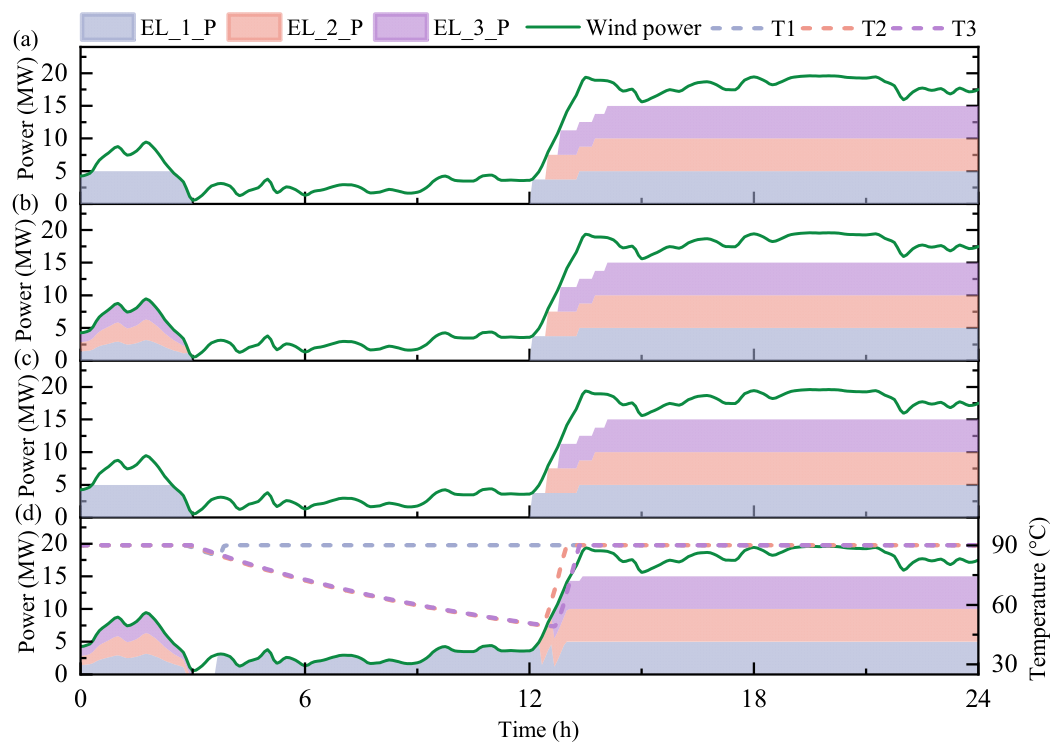
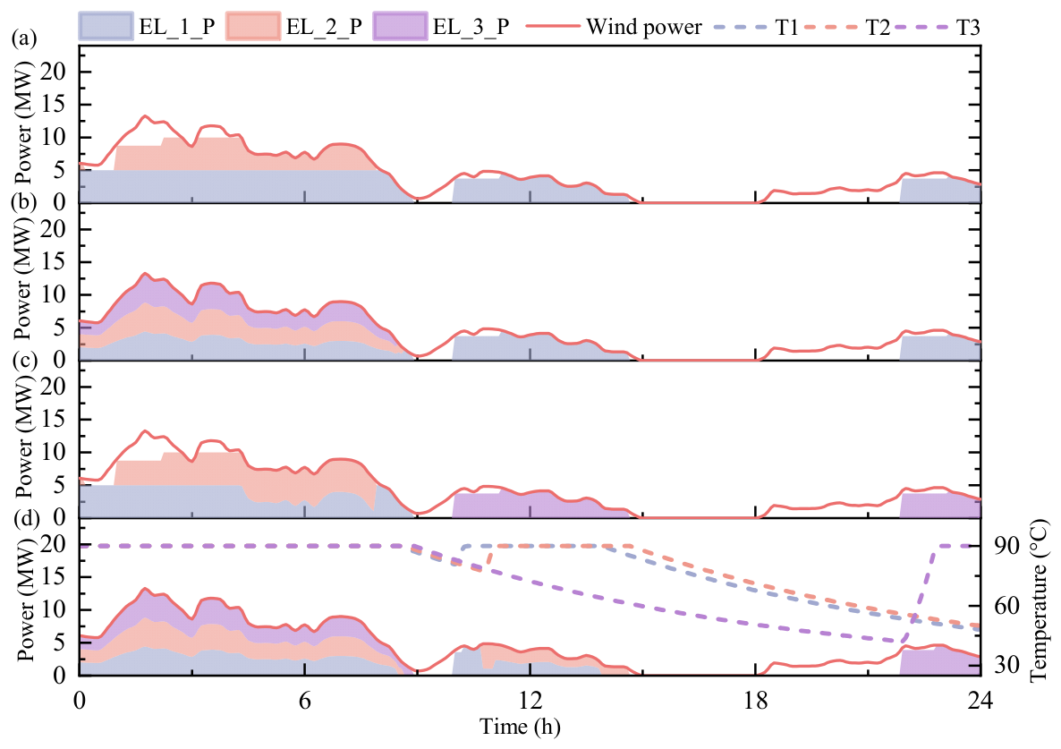
To evaluate the advantages of the proposed strategy, a comparative analysis was conducted on the dispatch results of the Daisy Chain strategy (Strategy 1), the Equal Allocation strategy (Strategy 2), the Rotation Control strategy (Strategy 3), and the Temperature–Power Adaptive strategy (Strategy 4) under typical seasonal daily wind power fluctuation scenarios. The dispatch results of the four strategies for the typical spring day are illustrated in Figure 8.

The wind power profile of this typical spring day is characterized by a “continuous ramp-up starting from a low power level”. As observed from the overall dispatch results, the power allocation and state transitions of Strategy 3 are identical to those of Strategy 1. From the perspective of the control strategy, this consistency in dispatch results occurs because the operational states of the three electrolyzers remain consistent for the majority of the time under this specific wind scenario. During the 0–3 h period, the wind power fluctuates at a median level and gradually decreases. Under the dispatch of Strategy 1, the initial wind power can only satisfy the production state requirement of Electrolyzer 1, and the subsequent fluctuating wind power is insufficient to start Electrolyzer 2, leading to wind curtailment during this period. Conversely, under Strategies 2 and 4, the initial wind power supports all three electrolyzers with input powers greater than the minimum operating power, keeping them all in the production state. Under conditions where wind power fluctuations do not trigger state transitions and the temperatures of all electrolyzers are identical, the power optimization results based on the nonlinear hydrogen production rate model indicate that the optimal power allocation method to maximize total system hydrogen production is the equal allocation of input power.

During the 3–12 h period, the wind power continuously fluctuates at a low level. Strategies 1, 2, and 3, which ignore the influence of temperature on the startup process, determine that the wind power cannot meet the electrolyzer startup requirements; thus, no electrolyzers are brought into the production state during this timeframe. In contrast, Strategy 4, based on the temperature–power adaptive relationship, determines that one electrolyzer can be started. Since all three electrolyzers have the same number of start–stop cycles, Electrolyzer 1, which entered the standby state first and has the shortest cumulative operating time, is prioritized for startup. After cooling for 10 time steps, the temperature of Electrolyzer 1 drops from 90 °C to 84.67 °C. Based on the temperature–power adaptive relationship corresponding to this initial temperature and the system input power, the optimized startup plan dictates a startup power of 3.00 MW, taking 527 s (2 time steps) to complete. Subsequently, the wind power fluctuation remains insufficient to support the startup of a second electrolyzer. Electrolyzer 1 operates in the low-power range, improving the utilization rate of renewable energy during this period. Physically, this process reflects the utilization of the electrolyzer’s thermal inertia. By relying on the retained sensible heat of the electrolyte, the energy demand for this hot start is reduced, which helps avoid wind curtailment.

During the 12–15 h period, the wind power rapidly and substantially ramps up from a low level. Strategies 1, 2, and 3 adopt a fixed startup power (3.76 MW) and startup duration (15 time steps) to sequentially start Electrolyzers 1, 2, and 3. Strategy 4, while ensuring Electrolyzer 1 maintains its production state, sequentially starts electrolyzers 2 and 3 based on their cumulative operating times. The initial startup temperature of Electrolyzer 2 is 49.72 °C. By combining the temperature–power adaptive relationship, the operational state of Electrolyzer 1, and the system input power, its optimal startup power is determined to be 4.32 MW, with the startup process taking 2348 s (8 time steps). When the startup conditions for Electrolyzer 3 are satisfied, it initiates startup at an initial temperature of 49.07 °C and a startup power of 4.30 MW, completing the process in 2412 s (9 time steps). Strategy 4 effectively shortens the startup time. Specifically, by sensing the low temperature of the standby electrolyzer and the rapid, substantial surge in wind power, the strategy allows Electrolyzer 1 (which is already producing) to proactively decrease its input power to create a power margin. Consequently, a constant-voltage startup mode is adopted. By utilizing the maximum startup power, the heating process is accelerated, minimizing total heat loss to the environment. Electrochemically, this faster temperature rise more quickly decreases the polarization overpotential, enabling the electrolyzer to reach an efficient hydrogen production state sooner, thereby further enhancing the wind power accommodation capacity.

Under the spring working condition of “continuous ramp-up starting from a low power level,” the performance comparison of each strategy is detailed in

Table 7. Operational indicators of different strategies for the typical spring day.

Performance Indicator	Strategy 1	Strategy 2	Strategy 3	Strategy 4
Wind power accommodation rate (%)	72.86	75.12	72.86	85.76
Total start–stop cycles	4	6	4	6
Total startup time (min)	215.75	215.75	215.75	88.12
Total startup energy consumption (MWh)	13.51	13.51	13.51	6.14
Average efficiency (%)	64.44	65.07	64.44	65.80
Total hydrogen production (Nm3)	3.60 × 104	3.76 × 104	3.60 × 104	4.32 × 104

.

Under Strategy 4 dispatch, the wind power accommodation rate and total hydrogen production increased by 17.7% and 20.0%, respectively, compared to Strategies 1 and 3, and by 14.2% and 14.9%, respectively, compared to Strategy 2. The core advantage lies in the dynamic process optimization: the total startup time and total startup energy consumption of the proposed strategy are less than half of those required by the traditional strategies (Strategies 1–3), reduced by approximately 59.2% and 54.6%, respectively. This comprehensively verifies the advantages of the temperature–power adaptive mechanism in accelerating system response and reducing startup costs. Physically, by decreasing the time the system operates in a low-temperature and high-resistance state, the adaptive strategy allows a larger proportion of the input electrical energy to be converted into chemical energy rather than being dissipated as Joule heat. This mechanism fundamentally contributes to the simultaneous enhancements in accommodation capacity, response speed, and overall operational energy efficiency.

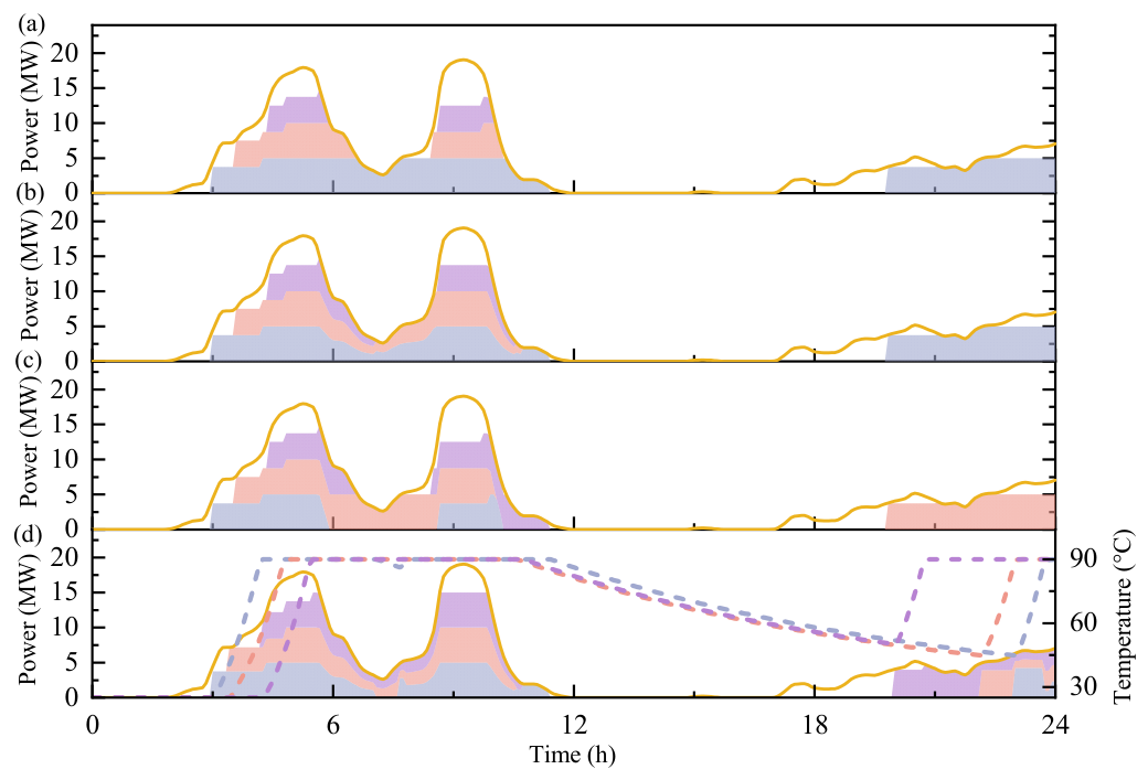
The dispatch results of the four strategies for the typical summer day are illustrated in Figure 9.

The wind power profile of this typical summer day exhibits the operational characteristic of “fluctuations in the medium–low power range accompanied by short-term wind lulls”. During the 0–9 h period, the wind power decays from a medium–high level to an extremely low level. Similar to the analysis conclusion for the 0–3 h period of the typical spring day, Strategies 1 and 3 adopt a sequential switching logic; they utilize the remaining power to start subsequent units only after the preceding electrolyzer reaches full load. Consequently, under identical conditions, Strategies 1 and 3 produce a more significant wind curtailment phenomenon compared to Strategies 2 and 4. Although the macroscopic power allocation and state transitions of Strategy 3 are identical to those of Strategy 1, their electrolyzer activation sequences differ significantly due to the dynamic priority rotation. Specifically, following the rotation at the 4 h mark, the priority sequence shifts to {2, 3, 1}. Therefore, during this period, Strategy 3 directs Electrolyzer 2 to operate at full load while Electrolyzer 1 absorbs the fluctuating power. Furthermore, during the 8–12 h and 20–24 h periods, the priority sequence updates to {3, 1, 2]. As a result, whenever the supplied power satisfies the startup conditions, Electrolyzer 3 is strictly prioritized for activation. This rule-based rotation effectively mitigates the severe fatigue accumulation concentrated on Electrolyzer 1 in Strategy 1.

During the 9–12 h period, the wind power slowly recovers from an extremely low level and enters a low-power fluctuation state. Strategies 1, 2, and 3 can only support the startup of a single electrolyzer. However, Strategy 4, based on the condition of higher real-time electrolyzer temperatures, determines that this low-power fluctuation interval can support the sequential startup of two electrolyzers. The initial startup temperature of Electrolyzer 1 is 80.72 °C. Based on the temperature–power adaptive relationship and the variation in system input power, its startup is completed in 730 s (3 time steps) with a startup power of 3.58 MW. Subsequently, Strategy 4 controls Electrolyzer 1 to actively reduce its input power to approach the minimum operating power limit, thereby releasing the necessary power margin so that the remaining wind power can support the startup of Electrolyzer 2. Under an initial temperature of 77.48 °C, Electrolyzer 2 completes its startup in 986 s (4 time steps) with a startup power of 3.78 MW.

Consistent with the physical mechanisms analyzed in the spring scenario, Strategy 4 proactively creates a power margin to facilitate startup. Because the initial temperatures remain high during these short-term wind lulls, the strategies effectively exploit the thermal inertia to execute rapid hot starts, thereby avoiding the severe thermal energy penalties associated with complete cooling. Afterwards, since the system input power is insufficient to start Electrolyzer 3 while ensuring Electrolyzers 1 and 2 maintain their production states, Electrolyzers 1 and 2 operate by equally sharing the fluctuating wind power. This dispatch method achieves the coordinated operation of multiple electrolyzers during low-power periods, improving the wind power accommodation rate and the overall hydrogen production efficiency of the system.

Under the summer working condition of “fluctuations in the medium–low power range accompanied by short-term wind lulls”, the performance comparison of each strategy is detailed in

Table 8. Operational indicators of different strategies for the typical summer day.

Performance Indicator	Strategy 1	Strategy 2	Strategy 3	Strategy 4
Wind power accommodation rate (%)	83.81	90.11	83.81	91.18
Total start–stop cycles	6	6	6	10
Total startup time (min)	215.75	143.83	215.75	81.88
Total startup energy consumption (MWh)	13.51	9.00	13.51	5.23
Average efficiency (%)	65.47	68.39	65.47	69.05
Total hydrogen production (Nm3)	1.82 × 104	2.05 × 104	1.82 × 104	2.09 × 104

.

In the typical summer scenario, the advantage of Strategy 4 in terms of total hydrogen production diminishes, but its advantage in the startup process remains significant. Although the total number of start–stop cycles increases to 10, the average efficiency maintains the highest level.

Physically, although frequent start–stop operations typically introduce severe thermal energy losses, the temperature-adaptive mechanism ensures these transitions occur primarily in the high-temperature zone. By leveraging the retained heat during short-term wind lulls, the strategy transforms potentially inefficient cold starts into flexible hot starts. This sustains a low polarization overpotential across the operational period, fundamentally explaining why the overall energy efficiency remains optimal despite the increased cycle count.

The dispatch results of the four strategies for the typical autumn day are illustrated in Figure 10.

The wind power profile of this typical autumn day is characterized by “intermittent fluctuations with a dual-peak structure”. During the 2–6 h period, the wind power experiences a process of climbing from zero to a peak and then rapidly declining. Strategies 1, 2, and 3 employ fixed startup powers and durations to sequentially start Electrolyzers 1, 2 and 3. In contrast, after starting Electrolyzer 1, the temperature–power adaptive strategy (Strategy 4) actively reduces its input power to release a power margin, enabling the subsequent electrolyzers to start earlier. Consistent with the physical mechanisms analyzed in the spring scenario, this mechanism not only shortens the overall time required to bring multiple electrolyzers into production but also improves the wind power accommodation rate during this period.

During the 6–12 h period, the wind power first passes through a trough, then rapidly climbs to a second peak, and drops again. During the trough period, Strategy 1 can only maintain Electrolyzer 1 in the production state; when the power recovers, it needs to restart Electrolyzers 2 and 3, resulting in low energy utilization. Furthermore, they must be taken offline again when the power drops, leading to frequent state transitions. Strategy 2 can maintain Electrolyzers 1 and 2 in the production state during the trough. Once the power increases and fully loads both units, the remaining power margin is used to start Electrolyzer 3. During the decline phase, all three electrolyzers equally share the system input power. For Strategy 3, based on the dynamic rotation sequence, Electrolyzers 1 and 3 are sequentially taken offline during the power trough. As the wind power recovers, a new rotation cycle updates the priority sequence to {1, 2, 3}. Given that Electrolyzer 2 has been maintained in the production state, Strategy 3 sequentially starts Electrolyzer 3 followed by Electrolyzer 1. Strategy 4, however, takes Electrolyzer 1 (the earliest to start) offline during the trough. When the power rapidly recovers, Strategy 4 exploits the thermal inertia of Electrolyzer 1. Because the electrolyte retains substantial sensible heat during the brief power trough, maintaining a relatively high initial temperature (86.22 °C), the electrolyzer completes a restart in only 475 s (2 time steps) with a startup power of 2.78 MW. This physically prevents a full cooling cycle and minimizes the thermal energy penalty associated with restarting. As the subsequent power drops from the peak, the three electrolyzers equally share the input power within their respective operating power ranges. Within this period, Strategy 4 exhibits the highest wind power accommodation rate and hydrogen production efficiency.

During the low-power fluctuation phase of 18–24 h, Strategies 1 and 3 can only support the startup and fluctuating operation of a single electrolyzer. Meanwhile, relying on the temperature–power adaptive relationship, Strategy 4 rapidly and sequentially starts all three electrolyzers under the low power level, enhancing the system’s ability to track and accommodate subsequent wind power fluctuations.

Under the autumn working condition of “intermittent fluctuations with a dual-peak structure”, the performance comparison of each strategy is detailed in

Table 9. Operational indicators of different strategies for the typical autumn day.

Performance Indicator	Strategy 1	Strategy 2	Strategy 3	Strategy 4
Wind power accommodation rate (%)	76.86	79.00	76.86	83.12
Total start–stop cycles	11	9	11	10
Total startup time (min)	215.75	143.83	215.75	81.88
Total startup energy consumption (MWh)	13.51	9.00	13.51	5.23
Average efficiency (%)	64.49	65.65	64.49	66.57
Total hydrogen production (Nm3)	1.66 × 104	1.74 × 104	1.66 × 104	1.85 × 104

.

In the typical autumn scenario, the total startup time and energy consumption of Strategy 4 are reduced by 62.1% and 61.3% compared to Strategies 1 and 3, and by 43.1% and 41.89% compared to Strategy 2. This once again verifies the core advantage of the temperature–power adaptive mechanism in significantly reducing the dynamic response cost of the electrolyzers when dealing with frequent and substantial power variations.

Physically, by preserving the sensible heat of the electrolyte during intermittent power drops, the strategy prevents the severe electrochemical penalty—specifically, the high polarization overpotential—associated with cold starts.

Although its advantage margin in wind power accommodation rate and total hydrogen production has decreased compared to the spring scenario, under the complex intermittent fluctuations of autumn, this strategy still achieves the highest average energy efficiency for the electrolyzer group. This indicates that maintaining a higher average operating temperature effectively minimizes Ohmic losses, maximizing the proportion of electrical input converted into chemical energy.

Furthermore, with a total number of start–stop cycles comparable to that of Strategy 2, it successfully strikes an optimal balance among accommodation capacity, operational energy efficiency, and dynamic response.

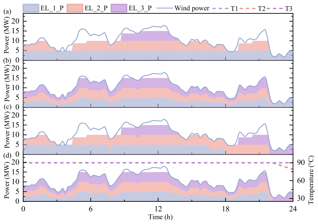
The dispatch results of the four strategies for the typical winter day are illustrated in Figure 11.

The wind power profile of this typical winter day is characterized by “continuous fluctuations within a high-power range and narrow amplitude”. Under such conditions, the multi-electrolyzer system is spared from frequent start–stop operations. Consequently, the temperature of each electrolyzer remains relatively stable. Strategy 4 and Strategy 2 exhibit identical dispatch performance in this scenario, both achieving stable power allocation and efficient accommodation.

In contrast, Strategies 1 and 3 are constrained by their sequential switching mechanisms. This limitation causes the electrolyzer ranked last in the priority sequence to bear the entirety of the power fluctuations, inducing unnecessary state transitions and wind curtailment phenomena. Although Strategy 3 avoids excessive fatigue of a single electrolyzer by rotating the priority sequence, it fails to improve energy utilization.

Under the winter working condition of “continuous fluctuations within a high-power range and narrow amplitude,” the performance comparison of each strategy is detailed in

Table 10. Operational indicators of different strategies for the typical winter day.

Performance Indicator	Strategy 1	Strategy 2	Strategy 3	Strategy 4
Wind power accommodation rate (%)	88.17	97.68	88.17	97.68
Total start–stop cycles	7	2	7	2
Total startup time (min)	215.75	0	215.75	0
Total startup energy consumption (MWh)	13.51	0	13.51	0
Average efficiency (%)	64.49	67.18	64.49	67.18
Total hydrogen production (Nm3)	4.35 × 104	4.99 × 104	4.35 × 104	4.99 × 104

.

The indicators for Strategy 4 and Strategy 2 are identical, with both significantly outperforming the sequential switching strategies (Strategies 1 and 3) in terms of wind power accommodation rate, hydrogen production, and system efficiency. In scenarios devoid of start–stop operations, the proposed strategy maintains optimal operational performance.

4. Discussion

Based on the comprehensive analysis of the case studies across four seasons, the core advantage of the proposed control strategy based on temperature–power adaptation lies in its response to “ultra-low power recovery” processes. According to the specific characteristics of power recovery, the response mechanism can be categorized into two scenarios:

(1)

During slow power recovery with continuous low-level fluctuations: The proposed strategy leverages the temperature–power adaptive relationship to identify feasible startup power windows that are lower than traditional fixed thresholds. By integrating decision-making regarding start–stop cycles and cumulative operating time, it determines the optimal startup target, thereby effectively utilizing low-power resources and improving the wind power accommodation rate.

(2)

During rapid and substantial power ramp-up: The proposed strategy actively regulates the power of operating electrolyzers closer to their lower limits to increase the system’s power margin, enabling subsequent electrolyzers to meet startup conditions earlier. Furthermore, by combining real-time temperature data to match the optimal startup power, it achieves the advancement and overlapping of startup processes for multiple electrolyzers. This mechanism significantly shortens the time required for the entire fleet to transition into the production state, ensuring efficient tracking of the power ramp-up.

5. Conclusions

This paper systematically investigates the impact mechanism of temperature variations on the dynamic operation of alkaline electrolyzers under fluctuating conditions, revealing the intricate coupling relationship among temperature, power, and time during the startup process. Integrated with a hierarchical optimization scheduling framework, a multi-electrolyzer control optimization strategy based on temperature–power adaptation is proposed. The effectiveness of this strategy was rigorously validated through simulations of typical seasonal scenarios. The primary findings of this study are summarized as follows:

• Temperature variations alter the operational characteristics of the electrolyzer through electro-thermal coupling, which has been accurately characterized via a quantitative model. The simulation analysis indicates that temperature is a critical variable dictating polarization characteristics, heat generation and dissipation, and the hydrogen production rate. Based on these findings, the startup time is derived as a bivariate function of the initial temperature and the startup power, thereby establishing the precise temperature–power adaptive relationship. This underlying relationship provides a solid foundation for accurate power optimization and allocation.
• A dual-layer optimization framework is constructed based on this quantitative relationship to achieve the adaptive control of multiple electrolyzers. In the proposed strategy, the upper-layer Mixed-Integer Linear Programming (MILP) model formulates state-switching and baseline power allocation plans derived from short-term forecasts. Correspondingly, the lower-layer rolling optimization, utilizing the Mongoose Optimization Algorithm (MOA), relies on ultra-short-term forecasts and the real-time temperatures of individual electrolyzers. By employing the adaptive relationship, it dynamically calibrates the startup process and power distribution, successfully balancing global macroscopic optimization with real-time control precision.
• Comparative simulations across typical seasonal scenarios quantitatively confirm the superiority of the proposed strategy. Taking the typical spring fluctuating scenario as an example, the proposed approach reduces total startup time by up to 59.2% and startup energy consumption by up to 54.6% compared to traditional control methods. Concurrently, it increases wind power accommodation by up to 17.7%, total hydrogen production by up to 20.0%, and average operational efficiency by up to 1.36%. By actively sensing the real-time temperatures of multiple electrolyzers to adaptively schedule state transitions and power allocation, the proposed strategy effectively overcomes the limitations of fixed startup models. Consequently, by strictly adhering to actual operational boundaries, it ensures the synergy and reliability required for safe and efficient large-scale hydrogen production under fluctuating conditions.

It should be noted that while the foundational thermodynamic and polarization models in this study were rigorously validated against experimental data from an actual 5 MW industrial alkaline electrolyzer, the validation of the overall control strategy currently relies on simulations. This limitation stems from the prohibitive hardware costs and physical constraints associated with deploying multiple megawatt-scale electrolyzers for system-level experimental testing. Therefore, in future work, a scaled-down experimental testbed or a Hardware-in-the-Loop (HIL) testing platform will be established. By deploying the proposed strategy onto physical controllers, its real-time hardware execution performance and reliability will be further validated.

References

1. Abdelsalam, R.A.; Mohamed, M.; Farag, H.E.Z.; El-Saadany, E.F. Green Hydrogen Production Plants: A Techno-Economic Review. Energy Conv. Manag. 2024, 319, 118907. [Google Scholar] [CrossRef] [Scilit]
2. Oussmou, B.; Sigue, S.; Abderafi, S. Review of Green Hydrogen Production Technologies, to Choose the Optimal Process of Electrolysis-Renewable Energy. Renew. Sust. Energy Rev. 2026, 225, 116205. [Google Scholar] [CrossRef] [Scilit]
3. Mohsen, F.M.; Mjbel, H.M.; Challoob, A.F.; Alkhazaleh, R.; Alahmer, A. Advancements in Green Hydrogen Production: A Comprehensive Review of Prospects, Challenges, and Innovations in Electrolyzer Technologies. Fuel 2026, 404, 136251. [Google Scholar] [CrossRef] [Scilit]
4. Eldeeb, H.H.; Abdelsalam, A.M.; Sakr, I.M.; El-Askary, W.A.; Farahat, M.A. Experimental Evaluation of a Modular Solar-Powered Alkaline Electrolyzer for Scalable Hydrogen Production. Fuel 2026, 405, 136802. [Google Scholar] [CrossRef] [Scilit]
5. Xu, Z.; Sun, L.; Xiao, J.; Wang, F.; Zhuo, F. Optimization Control of Wind Power Hydrogen Electrolyzer Array Considering the Operating Characteristics of Electrolyzer. High Volt. Eng. 2025, 51, 2175–2185. (In Chinese) [Google Scholar] [CrossRef]
6. Yang, X.; Yao, M.; Han, W.; Feng, P.; Zhang, K. Review on Current Status and Development of Large-Scale Renewable Energy Electrolysis Hydrogen Production Technology. Therm. Power Gener. 2025, 54, 33–43. (In Chinese) [Google Scholar] [CrossRef]
7. Mansouri, A.; Magri, A.E.; Lajouad, R.; Giri, F.; Watil, A. An Adaptive Non-Linear Control of a Wind Energy Conversion System Connected to an HVDC Line Involving a Vienna Rectifier. IFAC-PapersOnLine 2022, 55, 806–811. [Google Scholar] [CrossRef] [Scilit]
8. Watil, A.; Magri, A.E.; Lajouad, R.; Raihani, A.; Giri, F.; El Fadili, A.; Mansouri, A. A Power Balance Control Strategy for Stand Alone Wind Energy Conversion Systems. IFAC-PapersOnLine 2022, 55, 788–793. [Google Scholar] [CrossRef] [Scilit]
9. Corigliano, O.; Fragiacomo, P. Energy-Environmental Analysis of an H2PEM Power Station Assisted by a Dynamic Simulation Tool. Sustain. Energy Fuels 2025, 9, 2433–2465. [Google Scholar] [CrossRef] [Scilit]
10. Corigliano, O.; Genovese, M.; Fragiacomo, P. Dynamic Modeling and Simulation of a Hydrogen Power Station for Continuous Energy Generation and Resilient Storage. J. Power Sources 2025, 629, 236076. [Google Scholar] [CrossRef] [Scilit]
11. Xia, Y.; Wei, W.; Cheng, H.; Zhou, Y.; Zhao, B.; Zhang, L. Key Scientific Problems for Large-Scale Hydrogen Production from Alkaline Water Electrolyzers Directly Driven by Renewable Energy. Acta Energiae Solaris Sin. 2024, 45, 224–231. (In Chinese) [Google Scholar] [CrossRef]
12. Zhou, Z.; Zheng, M.; Dong, B.; Li, J. Cluster Allocation Strategy of Multi-Electrolyzers in Wind-Hydrogen System Considering Electrolyzer Degradation under Fluctuating Operating Conditions. Renew. Energy 2025, 242, 122381. [Google Scholar] [CrossRef] [Scilit]
13. Yang, F.; Yan, R.; Sun, H.; Lei, Z.; Liu, B. Feasible Domain Analysis and Multi-Objective Optimization of Operating Parameters for Alkaline Water Electrolysis Hydrogen Production under Fluctuating Operating Conditions. Trans. China Electrotech. Soc. 2025. (In Chinese) [Google Scholar] [CrossRef]
14. Gu, J.; Guo, B.; Hu, S.; Ding, S.; Zhang, T.; Tian, Z.; Yang, F.; Ouyang, M. Experimental Studies on Dynamic Performance of 250-kW Alkaline Electrolytic System. J. Power Sources 2024, 592, 233920. [Google Scholar] [CrossRef] [Scilit]
15. Hu, C.; Hu, X.; He, S.; Wang, L.; Shen, S. Research on Performance of a Filter-Press Alkaline Electrolyzer Coupled with Multiphysics Fields. Clean Coal Technol. 2025, 31, 230–242. (In Chinese) [Google Scholar] [CrossRef]
16. Ren, Z.; Wang, J.; Yu, Z.; Zhang, C.; Gao, S.; Wang, P. Experimental Studies and Modeling of a 250-kW Alkaline Water Electrolyzer for Hydrogen Production. J. Power Sources 2022, 544, 231886. [Google Scholar] [CrossRef] [Scilit]
17. Han, X.; Zhang, Z.; Liu, M. Optimization Control Method of Dual-Channel Hydrogen Production System with Multi-Power Scenarios Based on Petri Net. Acta Energiae Solaris Sin. 2025, 46, 142–151. (In Chinese) [Google Scholar] [CrossRef]
18. Li, Y.; Deng, X.; Zhang, T.; Liu, S.; Song, L.; Yang, F.; Ouyang, M.; Shen, X. Exploration of the Configuration and Operation Rule of the Multi-Electrolyzers Hybrid System of Large-Scale Alkaline Water Hydrogen Production System. Appl. Energy 2023, 331, 120413. [Google Scholar] [CrossRef] [Scilit]
19. Varela, C.; Mostafa, M.; Zondervan, E. Modeling Alkaline Water Electrolysis for Power-to-x Applications: A Scheduling Approach. Int. J. Hydrogen Energy 2021, 46, 9303–9313. [Google Scholar] [CrossRef] [Scilit]
20. Zhang, Y.; Zhang, F.; Song, X.; Chen, R.; Chen, Z.; Duan, X.; Xia, Y. Optimization of Multiple Alkaline Water Electrolyzers Coupled with Solar Photovoltaic Power for Green Hydrogen Production on a Large Scale. Int. J. Hydrogen Energy 2025, 136, 511–532. [Google Scholar] [CrossRef] [Scilit]
21. Zou, P.; Lin, H.; Zhou, X.; Zou, Y.; Li, Y.; Yan, G.; Duan, X.; Cai, J. Control Strategies for Multi-Electrolyzer Alkaline Hydrogen Generation Systems Improving Renewable Energy Utilization and Electrolyzer Lifespan. Renew. Energy 2025, 253, 123628. [Google Scholar] [CrossRef] [Scilit]
22. Zou, P.; Lin, H.; Zou, Y.; Zhou, X.; Liu, Z.; Duan, X.; Li, Y.; Chen, J.; Song, Y. Dynamic Scheduling of Renewable-Powered Multi-Electrolyzer Systems for Hydrogen Production with Simulated Annealing Optimization: A Load Balancing and Efficiency Enhancement Approach. Renew. Energy 2026, 258, 124967. [Google Scholar] [CrossRef] [Scilit]
23. Han, P.; Xu, X.; Wang, H.; Yan, Z. Operational Efficiency Enhancement of Multi-Stack Proton Exchange Membrane Electrolyzer Systems with Power-Temperature Adaptive Control. Trans. China Electrotech. Soc. 2024, 39, 2236–2248. (In Chinese) [Google Scholar] [CrossRef]
24. Zhang, X.; Bai, M.; Su, X.; Zhou, J. Power Adaptive Control Strategy Based on Optimal Efficiency of Hydrogen Production System. Acta Energiae Solaris Sin. 2025, 46, 126–135. (In Chinese) [Google Scholar] [CrossRef]
25. Qiu, Y.; Zhou, B.; Zang, T.; Zhou, Y.; Chen, S.; Qi, R.; Li, J.; Lin, J. Extended Load Flexibility of Utility-Scale P2H Plants: Optimal Production Scheduling Considering Dynamic Thermal and HTO Impurity Effects. Renew. Energy 2023, 217, 119198. [Google Scholar] [CrossRef] [Scilit]
26. Shen, X.; Nie, C.; Lü, H. Coordination Control Strategy of Wind Power-Hydrogen Alkaline Electrolyzer Bank Considering Electrothermal Characteristics. Trans. China Electrotech. Soc. 2021, 36, 463–472. (In Chinese) [Google Scholar] [CrossRef]
27. Sun, J.; Peng, Y.; Wang, A.; Feng, Q.; Wang, Y. Optimal Operation for P2H System Based on a Power-Temperature-Hydrogen Coupling Model for Alkaline Water Electrolyzer Plant. Int. J. Hydrogen Energy 2024, 79, 150–163. [Google Scholar] [CrossRef] [Scilit]
28. Rozzi, E.; Grimaldi, A.; Minuto, F.D.; Lanzini, A. Model Complexity and Optimization Trade-Offs in the Design and Scheduling of Hybrid Hydrogen-Battery Systems. Energy Conv. Manag. 2025, 344, 120306. [Google Scholar] [CrossRef] [Scilit]
29. Wang, X.; Meng, X.; Nie, G.; Li, B.; Yang, H.; He, M. Optimization of Hydrogen Production in Multi-Electrolyzer Systems: A Novel Control Strategy for Enhanced Renewable Energy Utilization and Electrolyzer Lifespan. Appl. Energy 2024, 376, 124299. [Google Scholar] [CrossRef] [Scilit]
30. Yang, F.; Lei, Z.; Liu, B.; Yan, R.; Dong, Y.; Sun, H. The Feasible Domain Analysis of Operating Parameters Considering Temperature Effects under Fluctuating Conditions and Coordinated Control of AWE System. Int. J. Hydrogen Energy 2025, 141, 163–175. [Google Scholar] [CrossRef] [Scilit]
31. Hu, S.; Guo, B.; Ding, S.; Yang, F.; Dang, J.; Liu, B.; Gu, J.; Ma, J.; Ouyang, M. A Comprehensive Review of Alkaline Water Electrolysis Mathematical Modeling. Appl. Energy 2022, 327, 120099. [Google Scholar] [CrossRef] [Scilit]
Figure 1. Operational states and state transition model of the alkaline electrolyzer.
Inventions 11 00041 g001
Figure 2. Model validation: (a) Electrochemical model; (b) Thermal model; (c) Hydrogen production rate model.
Inventions 11 00041 g002
Figure 3. Variations in power, temperature, and hydrogen production rate under different startup methods. The vertical dashed lines, color-coded to match Case 1, Case 2, and Case 3, indicate the end time points of the cold-start and hot-start processes for each startup method under the same operating conditions.
Inventions 11 00041 g003
Figure 4. Variations in power, temperature, and hydrogen production rate at different initial temperatures. The vertical dashed lines, color-coded to match the respective initial temperatures, indicate the completion time points of the cold-start and hot-start processes.
Inventions 11 00041 g004
Figure 5. Quantitative relationship among startup time, initial temperature, and startup power.
Inventions 11 00041 g005
Figure 6. Framework of the temperature–power adaptive dual-layer optimization strategy.
Inventions 11 00041 g006
Figure 7. Typical daily wind power profiles across the four seasons.
Inventions 11 00041 g007
Figure 8. Dispatch results of different strategies for the typical spring day: (a) Daisy Chain Control Strategy; (b) Equal Allocation Control Strategy; (c) Rotation Control Strategy; (d) Temperature–Power Adaptive Strategy. In the legend, EL_1_P, EL_2_P, and EL_3_P represent the allocated input powers of Electrolyzers 1, 2, and 3, respectively, while T1, T2, and T3 denote their corresponding operating temperatures.
Inventions 11 00041 g008
Figure 9. Dispatch results of different strategies for the typical summer day: (a) Daisy Chain Control Strategy; (b) Equal Allocation Control Strategy; (c) Rotation Control Strategy; (d) Temperature–Power Adaptive Strategy. In the legend, EL_1_P, EL_2_P, and EL_3_P represent the allocated input powers of Electrolyzers 1, 2, and 3, respectively, while T1, T2, and T3 denote their corresponding operating temperatures.
Inventions 11 00041 g009
Figure 10. Dispatch results of different strategies for the typical autumn day: (a) Daisy Chain Control Strategy; (b) Equal Allocation Control Strategy; (c) Rotation Control Strategy; (d) Temperature–Power Adaptive Strategy. In the legend, EL_1_P, EL_2_P, and EL_3_P represent the allocated input powers of Electrolyzers 1, 2, and 3, respectively, while T1, T2, and T3 denote their corresponding operating temperatures.
Inventions 11 00041 g010
Figure 11. Dispatch results of different strategies for the typical winter day: (a) Daisy Chain Control Strategy; (b) Equal Allocation Control Strategy; (c) Rotation Control Strategy; (d) Temperature–Power Adaptive Strategy. In the legend, EL_1_P, EL_2_P, and EL_3_P represent the allocated input powers of Electrolyzers 1, 2, and 3, respectively, while T1, T2, and T3 denote their corresponding operating temperatures.
Inventions 11 00041 g011