Risk Assessment of Distribution Network Based on Dirichlet Process Mixture Model and the Cumulant Method

Abstract

To address the increased operational risk in distribution network caused by the grid integration of distributed wind power, a distribution network risk assessment method that combines a Dirichlet process mixture model (DPMM) with the cumulant method (CM) is proposed, to achieve effective quantification of operational risk. Firstly, a DPMM is employed to cluster wind power output data, and adaptive kernel density estimation is introduced to construct a probabilistic model of wind power output, thereby improving local fitting accuracy. Secondly, uncertainties arising from wind generation and load are considered, and a probabilistic power flow model for the distribution network is established based on the CM and the Gram–Charlier series expansion, in order to obtain the probability distributions of state variables and branch power flows. Then, distribution entropy theory is introduced to quantify the severity of limit violations for state variables such as voltage and power, so that operational risk assessment is enabled. Finally, simulations are conducted on a modified IEEE 34-bus distribution test system, and the results demonstrate the effectiveness of the proposed method.

1. Introduction

With the widespread integration of distributed generation, the operation mode of power systems is undergoing profound changes. The complementary and coordinated relationship between distributed generation and the traditional bulk power grid supply mode is regarded as an effective approach, one that makes full use of existing resources and equipment and provides users with highly reliable and high quality electric power [1]. However, this transition is also accompanied by significant impacts on the operating state of the distribution network [2]. Firstly, the integration of distributed generation is accompanied by changes in the power flow characteristics of the traditional distribution network, and the distribution of network loads and the direction of current flow are thereby affected. Secondly, renewable energy sources such as wind and solar power are used as distributed generation, and power output is influenced by variations in external environmental conditions [3]. As a result, considerable uncertainty is introduced into generation output [4,5]. Under such conditions, problems such as reverse overloading and local voltage instability may be caused in the distribution network, and the security and stability of the power grid may therefore be threatened [6].

Against this background, risk assessment is regarded as a quantitative evaluation process of the likelihood of uncertain events and the possible consequences caused by such events in a system [7,8], and particular importance is attached to it in the analysis of distribution networks containing renewable energy sources such as wind and solar power. In view of the volatility and uncertainty of distributed generation, traditional deterministic power flow methods are unable to accurately reflect these complex and uncertain influencing factors. As a result, the actual operating state of the distribution network cannot be accurately predicted. Therefore, a risk assessment method based on probability theory is adopted, and potential risks can be identified and quantified more effectively. On this basis, decision makers are assisted in formulating more scientific and reliable operation and dispatch strategies, and the safe and stable operation of the distribution network is thereby ensured [9,10].

Power flow analysis methods based on probability theory are mainly classified into three categories. The first category is represented by simulation methods, and the Monte Carlo method is taken as a typical example [11,12]. High accuracy is provided by this method, and only weak dependence on distributional assumptions is involved. However, a large computational burden is introduced, and a slow convergence rate is exhibited. Therefore, the requirements of large scale assessment are difficult to be satisfied. Nevertheless, this method is usually adopted as a benchmark for comparison because reliable results are produced. The second category is represented by approximation methods [13,14], in which estimation methods are commonly used. Through approximate inference of random variables and statistical quantities, computational complexity can be significantly reduced, and the time cost caused by extensive sampling can be avoided. However, approximation accuracy and scope of application are limited by linearization and distributional assumptions. The third category is represented by analytical methods [15,16], among which the cumulant method (CM) is taken as a representative one. Through the CM of input random variables, the probabilistic distribution characteristics of output variables are estimated, and probabilistic power flow analysis under high dimensional uncertainty is thereby made applicable. In distribution networks containing renewable energy sources, correlated superposition characteristics are exhibited by source and load uncertainties. Additivity is possessed by the CM, and the influences of multi-source random power injections on the statistical characteristics of voltage and power flow can therefore be conveniently integrated. Accordingly, probabilistic power flow assessment can be carried out by using the CM. In Ref. [17], the CM is applied to probabilistic power flow calculation in distribution networks, and the probability of voltage limit violation, together with its severity, is jointly used to characterize the risk of voltage limit violation after the integration of renewable energy sources. Refs. [18,19] conduct probabilistic power flow analysis by combining the Cornish–Fisher series expansion with the CM. In Ref. [18], risk indices for voltage limit violations and power flow limit violations are quantitatively provided. In Ref. [19], after the probability distributions of limit violations for nodal voltages and branch power flows are obtained, risk evaluation indices for voltage limit violations and branch current limit violations are constructed on the basis of utility theory. Refs. [20,21] employ the Gram–Charlier series expansion combined with the CM for probabilistic power flow and risk assessment. Ref. [20] proposes a probabilistic security assessment method for loop-closing operations by integrating Latin hypercube sampling (LHS) with the CM, using the cumulative probability distribution of loop-closing currents, the preliminary loop-closing success rate, and the severity of current limit violations as assessment indices. Ref. [21] establishes an evaluation system that includes the average probability of system voltage limit violations, the confidence interval of nodal voltages, and the nodal voltage exponential entropy. However, the risk indices in Refs. [17,18,19,20,21] mainly focus on results such as the probability of limit violations and the magnitude of limit violations. The uncertainty associated with the probability distribution of state variables, corresponding to risk, has not yet been incorporated into the evaluation. The consideration of risk factors remains insufficiently comprehensive.

In addition, the probability distribution of distributed renewable energy output needs to be accurately characterized, since this is regarded as the foundation of risk assessment. Existing distribution fitting methods are mainly divided into two categories. These categories are parameter estimation [22,23,24,25] and non-parametric estimation [26,27,28,29]. Refs. [22,23,24,25] employ parameter estimation for modeling. The output characteristics of renewable energy are commonly fitted by the Weibull distribution or the Beta distribution. However, this type of method relies on a prespecified distribution form. Model mismatch is therefore likely to occur. As a result, the evaluation accuracy of probabilistic power flow and risk indices is affected. By contrast, non-parametric estimation is not constrained by a specific distribution assumption. Statistical regularities can be directly extracted from historical data. This approach is therefore more suitable for characterizing complex distribution features, including multimodality and skewness. Related studies predominantly employ kernel density estimation (KDE) to establish probabilistic models for distributed generation and wind and solar output, or further construct wind, solar, and load joint distributions based on KDE for scenario generation through sampling [30,31]. However, renewable energy output distributions often exhibit pronounced local fluctuations. It is difficult for fixed bandwidth KDE to simultaneously capture local features at different power levels. Consequently, oversmoothing or undersmoothing is likely to be caused in power intervals where the density changes sharply. To address this issue, prior work has introduced adaptive KDE to enhance local fitting capabilities [32,33].

Although progress is achieved in distribution characterization by the above methods, the KDE usually relies on a relatively large sample size to ensure fitting quality. As a result, the burden of data processing is increased to a certain extent, and the efficiency of uncertainty analysis is constrained. To address this, some studies [34,35] have introduced Gaussian mixture models to cluster samples, with probability density estimation performed within each cluster, and the overall distribution reconstructed with weights to characterize local probability features under different output characteristics. However, this method requires presetting the number of clusters, and an inappropriate choice of cluster count may introduce distribution fitting bias.

In summary, a distribution entropy theory based risk assessment method for distribution networks is proposed in this paper. The innovations of this paper are as follows:

(1)

A Dirichlet process mixture model (DPMM) is introduced to perform Bayesian non-parametric clustering on wind power output samples, thereby avoiding the need to prespecify the number of clusters. In addition, adaptive KDE is employed within each cluster for probability density fitting, so that the accuracy of local fitting is improved.

(2)

For the random fluctuations of wind power and load in distribution networks, a probabilistic power flow solution method is constructed by combining the CM with the Gram–Charlier series expansion, through which the probabilistic distribution descriptions of nodal state variables and branch power flows are obtained.

(3)

Risk evaluation indices for the distribution network are constructed based on distribution entropy. These indices are used to characterize the risk of limit violations in state variables, such as voltage and power flow, as well as the risk caused by distribution uncertainty. Finally, the proposed method is validated on the improved IEEE 34-bus system, and the results provide a basis for operational risk analysis and dispatch decision making in distribution network.

2. Materials and Methods

2.1. Dirichlet Process Mixture Model

Wind power exhibits non-normal characteristics, such as randomly distributed density peaks and irregular shapes. Therefore, its statistical regularities are difficult to be effectively characterized by traditional modeling methods based on the normal distribution assumption. Furthermore, the distribution features, distribution parameters, and structure of wind power data are difficult to be determined in advance. The DPMM is characterized by non-parametric modeling capability. The cluster structure in data can be adaptively determined without prespecifying the number of categories. Additionally, high dimensional uncertain information can be effectively extracted. Therefore, the DPMM is suitable for the clustering analysis and probability density estimation of wind power.

It is assumed that the observed data are drawn from a mixed distribution $F\left(\theta \right)$ composed of several unknown categories. In this paper, wind power output data $x=\left[x_1,x_2,\cdots ,x_i,\cdots ,x_n\right]$ are selected as the data to be clustered. It is further assumed that these data follow a distribution with a set of parameters $\left\{{\theta }_1,{\theta }_2,\cdots ,{\theta }_i,\cdots ,{\theta }_n\right\}$, where n denotes the number of data points. Data associated with the same parameter θ are assigned to the same category. Accordingly, the wind power output data x to be clustered are ultimately divided into k categories, where k denotes the number of categories, n denotes the total number of data points, and k < n.

In this process, the parameter θ is assumed to be drawn from the Dirichlet process (DP). A mechanism for generating infinitely many potential categories is defined by the DP. As the amount of data increases, a category can be adaptively assigned to each observed sample without prespecifying the number of categories. More specifically, the DP is defined as a stochastic process of probability distributions on a measure space. A probability is assigned by this process to each possible category, and the number of categories is determined by the data itself rather than being specified in advance. Formally, let G denote a random probability distribution on a measure space. Let the measure space be arbitrarily partitioned into a = {a₁, a₂, …, a_r}. It is assumed that $G\left(a_1\right),G\left(a_2\right),\cdots ,G\left(a_r\right)$ follows the Dirichlet distribution, which is expressed as follows:

$$\left(G\left(a_1\right),G\left(a_2\right),\cdots ,G\left(a_r\right)\right)~\mathrm{Dir}\left({\alpha }_0{G}_0\left(a_1\right),{\alpha }_0{G}_0\left(a_2\right),\cdots ,{\alpha }_0{G}_0\left(a_r\right)\right)$$

(1)

where α₀ is a hyperparameter, and α₀ > 0, representing the degree of dispersion of G; G₀ is the base distribution.

This process can be defined as DP(α₀, G₀). The Dirichlet distribution is taken as the conjugate prior of the multinomial distribution. This means that, when the prior distribution is given by the Dirichlet distribution and the likelihood function follows the multinomial distribution, the posterior distribution is still given by the Dirichlet distribution. The clustering property is thus exhibited. For the DP, it is assumed that observed values $\left\{{\theta }_1,{\theta }_2,\cdots ,{\theta }_n\right\}$ are obtained by sampling from G. Then, the posterior distribution of these observed values satisfies the following form:

$$\begin{array}{l}P\left(G\left(a_1\right),G\left(a_2\right),\cdots ,G\left(a_r\right)\left|N_1,N_2,\cdots ,N_i,\cdots ,N_n\right.\right)~\\ \mathrm{Dir}\left({\alpha }_0{G}_0\left(a_1\right)+N_1,{\alpha }_0{G}_0\left(a_2\right)+N_2,\cdots ,{\alpha }_0{G}_0\left(a_r\right)+N_r\right)=\\ \mathrm{DP}\left({\alpha }_0+N,\left({\alpha }_0{G}_0+{\displaystyle \sum _{i=1}^n{\delta }_{{\theta }_i}}\right)/{\alpha }_0+N\right)\end{array}$$

(2)

where P is the probability of occurrence; $N_i$ is the number of observed values ${\theta }_i$; ${\delta }_{{\theta }_i}$ is the Dirac function of ${\theta }_i$; N is the total number of observations.

Since direct sampling cannot be performed from the DP, the Chinese restaurant process (CRP) is adopted in this paper to construct the random probability distribution G. In this model, the restaurant is assumed to contain infinitely many tables. The ith customer entering the restaurant is denoted by x_i, and the tables available to the customers are denoted by ${\varphi }_k$. The base distribution G₀ and the parameter ${\varphi }_k$ are used to represent the parameter of the kth table, respectively. When the x_ith customer enters the restaurant, the number of customers already seated at table ${\varphi }_k$ is denoted by mk. The ith customer is assigned to table ${\varphi }_k$ with a probability proportional to m_k, or is assigned to a new table with a probability proportional to ${\alpha }_0$. Accordingly, the table assignment of customers can be expressed as follows:

$$z_1,z_2,\cdots ,z_i,\cdots ,z_n:\mathrm{CRP}({\alpha }_0)$$

(3)

where the indicator variable z_i is used to represent the table assigned to the ith customer.

The specific process of CRP is shown in Algorithm 1.

Algorithm 1 Calculation Process for CRP.
1	Initialize a restaurant.
2	The first customer entering the restaurant is assigned to the kth table. An order is then placed. The same table can also be chosen by other customers for dining.
3	The second customer enters the restaurant with probability ${\alpha }_0/\left(1+{\alpha }_0\right)$ of choosing a new table, or probability $1/\left(1+{\alpha }_0\right)$ of sharing the same table as the first customer.
4	Until the (n + 1)th customer enters the restaurant, they choose table k with probability $P\left(z_{n+1}=k\left|z_{1:n}\right.\right)=m_k/\left({\alpha }_0+n\right),$ or choose a new table with probability ${\alpha }_0/\left(n+{\alpha }_0\right).$

Although the DP exhibits favorable clustering properties, its clustering mechanism is based on the consistency of parameter values. Therefore, it can only assign observations with the same parameter value to the same cluster, making it difficult to handle data that are numerically different but highly similar. To overcome this limitation, the DP is extended to the DPMM. The definition of DPMM can be expressed as follows:

$$\left\{\begin{array}{l}{x}_i\left|{\theta }_i:F\left({\theta }_i\right)\right.\\ {\theta }_i\left|G:G\right.\\ G\left|{\alpha }_0,G_0\right.:DP\left({\alpha }_0,G_0\right)\end{array}\right.$$

(4)

The DPMM constructed using the CRP is applied to cluster wind power output data. The DPMM model based on the CRP can be expressed as follows:

$$\left\{\begin{array}{l}{\theta }_k=\left({\mu }_k,{\sigma }_k^2\right):G_0\\ z_i\left|z_{-i}\right.:\mathrm{CRP}\left({\alpha }_0\right)\\ x_i\left|z_i\right.:N\left({\mu }_{z_i},{\sigma }_{z_i}^2\right)\end{array}\right.$$

(5)

where $N\left(\cdot \right)$ is the Gaussian distribution; ${\mu }_k$ and ${\sigma }_k^2$ are the mean and variance.

Subsequently, the following formula was further derived.

For an existing cluster k, given the parameters of cluster k, the conditional probability of sample x_i can be expressed as follows:

$$P\left(x_i\left|z_i=k,x_{-i}\right.\right)=N\left(x_i\left|{\mu }_k^{*},{\displaystyle \frac{{\sigma }_k^{*2}}{m_k^{*}+1}}\right.\right)$$

(6)

where ${\mu }_k^{*}$ and ${\sigma }_k^{*2}$ are the posterior mean and variance of cluster k, updated based on the observed data; $m_k^{*}$ is the updated sample size of cluster k.

The conditional probability for the new cluster k + 1 can be expressed as follows:

$$P\left(x_i\left|z_i=k+1\right.\right)=N\left(x_i\left|{\mu }_0,{\displaystyle \frac{{\sigma }_0^2}{m_0+1}}\right.\right)$$

(7)

where ${\mu }_0$ and ${\sigma }_0^2$ are the prior mean and variance of the new cluster; $m_0$ is the prior sample count of the new cluster.

After calculating the conditional probability, the Gibbs sampling algorithm is used to update the category assignment for each sample. Through multiple iterations, the algorithm eventually converges to the optimal category assignment.

2.2. Adaptive Kernel Density Estimation

The wind power output data used in this paper are characterized by complex distribution features, such as multimodality and significant skewness. In the KDE, the probability distribution is characterized directly on the basis of sample features, without prespecifying the distribution form of the data. The bandwidth parameter h is used to control the degree of smoothing of the kernel function. The specific expression is given as follows:

$$f\left(x;h\right)={\displaystyle \frac{1}{n}}{\displaystyle \sum _{i=1}^{n}K\left(x,x_i;h\right)}={\displaystyle \frac{1}{nh}}{\displaystyle \sum _{i=1}^{n}K\frac{\left(x-x_i\right)}{h}}$$

(8)

where $K\left(\cdot \right)$ is the kernel function. In this paper, the Gaussian function is selected as the kernel function.

However, the selection of the bandwidth is crucial to the accuracy of distribution fitting. If the bandwidth is too small, the estimation result becomes excessively sensitive, and overfitting is likely to be caused. If the bandwidth is too large, the details of distribution fitting cannot be accurately described. In addition, a fixed bandwidth is used in the traditional KDE method. Adaptive adjustment cannot therefore be performed according to the KDE value of each wind power output point. The flexibility of local fitting is thus restricted. As a result, overfitting or underfitting can still be caused when the data points are relatively concentrated or relatively dispersed.

To address the above problems existing in the traditional KDE algorithm based on wind power output, an adaptive non-parametric KDE method is proposed in this paper. Different bandwidths can be calculated according to each wind power output value. The specific method is given as follows.

An adaptive bandwidth factor is introduced:

$$\left\{\begin{array}{l}{\lambda }_i={\left[{\displaystyle \frac{p\left(x_i\right)}{{\displaystyle \prod _{i=1}^{n}p\left(x_i\right)}}}\right]}^{-\alpha }\\ p\left(x_i\right)={\displaystyle \frac{z_i}{{\displaystyle \sum _{i=1}^n{z}_i}}}\end{array}\right.$$

(9)

where α is the sensitivity factor and is set to 0.5 in this paper, a commonly used value in adaptive non-parametric KDE methods that balances overfitting and underfitting [36,37,38]; z_i is the number of occurrences for wind power output value x_i; p(x_i) is the probability of occurrence for wind power output value x_i.

By substituting Equation (9) into Equation (8), the adaptive non-parametric KDE formula can be obtained, as shown in Equation (10).

$$\widehat{f}\left(x;h\right)={\displaystyle \frac{1}{nh{\lambda }_i}}{\displaystyle \sum _{i=1}^{n}K\frac{\left(x-x_i\right)}{h{\lambda }_i}}$$

(10)

The cumulative distribution function (CDF) of wind power output is further obtained as follows:

$$F\left(x\right)={\displaystyle {\int }_0^x\widehat{f}\left(x\right)dx}$$

(11)

Finally, each category of wind power output obtained after clustering by the DPMM can be fitted by adaptive non-parametric KDE.

2.3. Risk Assessment Method for Distribution Network

In this paper, probabilistic power flow calculation is carried out for distribution network with distributed wind power, by combining the CM with the Gram–Charlier series expansion method. Subsequently, the limit violation conditions of branch probabilistic power flow and voltage probability are quantified based on distribution entropy theory, so that the risk of the distribution network can be evaluated.

2.3.1. Cumulant Method

The CM is a numerical characteristic of a random variable [39]. It is commonly used to quantify the downside risk associated with deviation from the expected value. Its definition is given as follows. Let $F\left(x\right)$ denote the distribution function of random variable x, and let t denote a real number, with $\left|e^{itx}\right|=1$. Then, function $g\left(x\right)=e^{itx}$ is integrable with respect to $F\left(x\right)$ over the interval from (−∞, +∞). The relation between this function of real variable t and the characteristic function of the distribution of F is given as follows:

$$\phi \left(t\right)=E\left(e^{itx}\right)={\displaystyle {\int }_{-\infty }^{+\infty }{e}^{itx}}dF\left(x\right)={\displaystyle {\int }_{-\infty }^{+\infty }{e}^{itx}f\left(x\right)}dx$$

(12)

where $E\left(e^{itx}\right)$ is the characteristic function of the random variable; f(x) is the probability density function of x.

By taking the natural logarithm of the characteristic function in Equation (12), and expanding its Maclaurin series in the neighborhood where t takes a relatively small value, the following expression can be obtained:

$$\ln \phi \left(t\right)=1+{\displaystyle \sum _{k=1}\frac{{\tau }_v}{v!}{\left(it\right)}^v+o\left(t^k\right)}$$

(13)

where ${\tau }_v$ is the vth order cumulant of the random variable; $o\left(t^k\right)$ is the remainder term of the expansion.

In power flow calculation, the perturbations of these random variables need to be introduced into the state variables of the system. By using the voltage sensitivity relationship, the linearized equations between state variables, such as nodal voltage and branch power flow, and nodal injected power can be obtained respectively, as shown below:

$$\left\{\begin{array}{c}\left[P_{\mathrm{node},\mathrm{base}},Q_{\mathrm{node},\mathrm{base}}\right]+\left[\Delta P_{\mathrm{node}},\Delta Q_{\mathrm{node}}\right]=\hfill \\ \hfill F_{\mathrm{volt}}\left(V_{\mathrm{base}},{\theta }_{\mathrm{base}}\right)+J_0\left[\Delta V,\Delta \theta \right]\\ \left[P_{\mathrm{line},\mathrm{base}},Q_{\mathrm{line},\mathrm{base}}\right]+\left[\Delta P_{\mathrm{line}},\Delta Q_{\mathrm{line}}\right]=\hfill \\ \hfill F_{\mathrm{line}}\left(V_{\mathrm{base}},{\theta }_{\mathrm{base}}\right)+G_0\left[\Delta V,\Delta \theta \right]\end{array}\right.$$

(14)

where $P_{\mathrm{node},\mathrm{base}}$ and $Q_{\mathrm{node},\mathrm{base}}$ are the reference expected values of nodal injected active power and reactive power; $P_{\mathrm{line},\mathrm{base}}$ and $P_{\mathrm{line},\mathrm{base}}$ are the reference expected values of line transmitted active power and reactive power; $P_{\mathrm{line},\mathrm{base}}$ and $\Delta Q_{\mathrm{node}}$ are the random perturbations of nodal injected active power and reactive power; $\Delta P_{\mathrm{line}}$ and $\Delta Q_{\mathrm{line}}$ are the random perturbations of branch active power and reactive power; $V_{\mathrm{base}}$ and ${\theta }_{\mathrm{base}}$ are the reference expected values of nodal voltage and phase angle; $F_{\mathrm{volt}}\left(\cdot \right)$ and $F_{\mathrm{line}}\left(\cdot \right)$ are the power flow equations of nodal injection and branch power; $J_0$ is the Jacobian matrix obtained from deterministic power flow calculation; $G_0$ is the sensitivity matrix; $\Delta V$ and $\Delta \theta$ are the variations in nodal voltage and phase angle.

By substituting the random perturbation values of nodal injected power into Equation (14), the cumulants of each order for state variables, such as nodal voltage and branch power flow, can be calculated through convolution, as shown in Equation (15):

$$\left\{\begin{array}{l}{\left[\Delta P_{\mathrm{line}},\Delta Q_{\mathrm{line}}\right]}_v={\left(G_0{J}_0^{-1}\right)}^v{\left[\Delta P_{\mathrm{node}},\Delta Q_{\mathrm{node}}\right]}_v\\ {\left[\Delta V,\Delta \theta \right]}_v={\left(J_0^{-1}\right)}^v{\left[\Delta P_{\mathrm{node}},\Delta Q_{\mathrm{node}}\right]}_v\end{array}\right.$$

(15)

In this paper, the random variables of nodal injected power are composed of load, conventional generating unit output, and wind power output. The CM is employed to derive the cumulants of each order. The specific procedure is given as follows:

(1)

Method for solving load cumulants

Due to the lack of load sample data, a normal distribution is adopted to model load uncertainty. Accordingly, the first-order and second-order cumulants are given by the mathematical expectation and variance, respectively, while the third-order and higher-order cumulants are taken as zero. This treatment preserves the main statistical characteristics of the load while maintaining the analytical efficiency of the cumulant method and the Gram–Charlier expansion method. The specific expressions are given as follows:

$$\left\{\begin{array}{l}{\tau }_{\mathrm{load},1}={\mu }_{\mathrm{load}}\\ {\tau }_{\mathrm{load},2}={\sigma }_{\mathrm{load}}^2\\ {\tau }_{\mathrm{load},3}={\tau }_{\mathrm{load},4}={\tau }_{\mathrm{load},5}=\cdots =0\end{array}\right.$$

(16)

(2)

Method for solving cumulants of conventional generating units

Traditional generating units are usually characterized by only two states, namely, operation and outage. It is assumed that the probability of a unit being in the operating state is p, while the probability of a unit being in the outage state is 1 − p. If Q generating units are included in the distribution network, and the probability that q units operate normally is p_q, the following conclusion can be obtained:

$$p_q={\widehat{P}}_Q^q{p}^q{\left(1-p\right)}^{Q-q}$$

(17)

All order moments of output power for the Q conventional generating units are given as follows:

$${\alpha }_{\mathrm{gen},v}=p_1{\widehat{P}}^v+p_2{\left(2\widehat{P}\right)}^v+\cdots +p_Q{\left(Q\widehat{P}\right)}^v$$

(18)

where $\widehat{P}$ is the rated capacity of the conventional generating unit.

(3)

Method for solving wind power cumulants

To reduce the influence of the randomness of wind power output on its distribution, a sampling method is employed in this paper to calculate the cumulants of wind power output. First, by combining the DPMM with adaptive non-parametric KDE, the probability density functions of wind power output under different categories are obtained. Then, the N wind power output data $\left\{P_{\mathrm{w},1},P_{\mathrm{w},2},P_{\mathrm{w},3},\cdots ,P_{\mathrm{w},N}\right\}$ are sampled by using the LHS method. Under the constant power factor control mode, the active power and reactive power of wind power are proportional. Corresponding reactive power data $\left\{Q_{\mathrm{w},1},Q_{\mathrm{w},2},Q_{\mathrm{w},3},\cdots ,Q_{\mathrm{w},N}\right\}$ can thus be obtained. Finally, on the basis of the origin moment theorem, the moments about the origin of each order for wind power output are further calculated:

$$\left\{\begin{array}{l}{\alpha }_{\mathrm{wind},v}^P={\displaystyle \frac{1}{N}}{\displaystyle \sum _{i=1}^N{P}_{\mathrm{wind},i}^v}\\ {\alpha }_{\mathrm{wind},v}^Q={\displaystyle \frac{1}{N}}{\displaystyle \sum _{i=1}^N{Q}_{\mathrm{wind},i}^v}\end{array}\right.$$

(19)

where ${\alpha }_{\mathrm{wind},v}^P$ and ${\alpha }_{\mathrm{wind},v}^Q$ are the vth order moments about the origin of the active power and reactive power of wind power output.

The relation between moments about the origin and cumulants is given in Equation (20). By calculating the moments about the origin, the cumulants of wind power output can be further obtained:

$$\ln \phi \left(t\right)=\log \left(1+{\displaystyle \sum _{k=1}\frac{{\alpha }_v}{v!}{\left(it\right)}^v}\right)=1+{\displaystyle \sum _{k=1}\frac{{\tau }_v}{v!}{\left(it\right)}^v+o\left(t^k\right)}$$

(20)

Furthermore, after the moments of each order for the wind power output random variable are estimated, the cumulants are further derived and calculated from these moments. The specific expressions are given as follows:

$$\left\{\begin{array}{ll}{\tau }_v={\alpha }_1,& \hfill v=1\\ {\tau }_v={\alpha }_v-{\displaystyle \sum _{i=1}^{v-1}{C}_{v-1}^i{\alpha }_i{\tau }_{v-1}},& \hfill v>1\end{array}\right.$$

(21)

where $C_{v-1}^i$ is the combination of selecting the i wind power output data points from v − 1 different wind power output data.

2.3.2. Gram–Charlier Series Expansion Method

The Gram–Charlier series expansion is a series approximation method based on the standard normal distribution. In this method, correction terms are constructed by using the cumulants of each order for a random variable. In this way, the probability density function (PDF) and the CDF of the random variable can be approximately obtained.

Let the expectation of random variable P be μ_P, and let the standard deviation be σ_P. A standardized random variable P’ is then obtained by standardization through $P^{\prime }=\left(P-{\mu }_P\right)/{\sigma }_P$. On the basis of the Type A Gram–Charlier series expansion, the probability density function and the cumulative distribution function of P′ can be further obtained. The expressions are given as follows:

$$f_{P^{\prime }}\left(P^{\prime }\right)=\varphi \left(P^{\prime }\right)+{\displaystyle \frac{A_1{\varphi }^{\left(1\right)}\left(P^{\prime }\right)}{1!}}+\cdots +{\displaystyle \frac{A_N{\varphi }^{\left(N\right)}\left(P^{\prime }\right)}{N!}}$$

(22)

$$F_{P^{\prime }}\left(P^{\prime }\right)={\displaystyle {\int }_{-\infty }^{+\infty }\varphi \left(P^{\prime }\right)d{P}^{\prime }+\frac{A_1\varphi \left(P^{\prime }\right)}{1!}+\cdots +\frac{A_N{\varphi }^{\left(N-1\right)}\left(P^{\prime }\right)}{N!}}$$

(23)

where $\varphi \left(\cdot \right)$ is the PDF of a random variable following the standard normal distribution; ${\varphi }^{\left(N\right)}\left(\cdot \right)$ is the Nth order derivative of $\varphi \left(\cdot \right)$; $A_1,\cdots ,A_N$ are the coefficients of the Gram–Charlier series expansion, which are calculated by Equation (24):

$$\left\{\begin{array}{l}{A}_1=0,A_2=0,\\ A_3=-{\tau }_{P^{\prime }}^{\left(3\right)},A_4={\tau }_{P^{\prime }}^{\left(4\right)},\\ A_5=-{\tau }_{P^{\prime }}^{\left(5\right)},A_6={\tau }_{P^{\prime }}^{\left(6\right)}+10{\left({\tau }_{P^{\prime }}^{\left(3\right)}\right)}^2,\\ A_7=-\left({\tau }_{P^{\prime }}^{\left(7\right)}+35{\tau }_{P^{\prime }}^{\left(3\right)}{\tau }_{P^{\prime }}^{\left(4\right)}\right),\\ A_8={\tau }_{P^{\prime }}^{\left(8\right)}+56{\tau }_{P^{\prime }}^{\left(3\right)}{\tau }_{P^{\prime }}^{\left(5\right)}+35{\left({\tau }_{P^{\prime }}^{\left(4\right)}\right)}^2\end{array}\right.$$

(24)

where ${\tau }_{P^{\prime }}^{\left(v\right)}$ is the vth order cumulant of the standardized random variable.

To summarize the steps above: first, the vth order cumulant ${\tau }_P^{\left(v\right)}$ of random variable P is calculated. Then, ${\tau }_{P^{\prime }}^{\left(v\right)}$ is obtained by using the linear property of cumulants. Finally, by substituting the results into Equations (22) and (23), $f_{P^{\prime }}\left(P^{\prime }\right)$ and $F_{P^{\prime }}\left(P^{\prime }\right)$ of the standardized random variable P’ can be obtained.

In addition, $f_{P^{\prime }}\left(P^{\prime }\right)$ and $F_{P^{\prime }}\left(P^{\prime }\right)$ of the standardized random variable P’ need to be restored by inverse standardization, so that the distribution result of the original random variable P can be obtained. The calculation process is given by the following expressions:

$$F_P\left(P\right)=P\left({\sigma }_P{P}^{\prime }+{\mu }_P\le P\right)=P\left(P^{\prime }\le {\displaystyle \frac{P-{\mu }_P}{{\sigma }_P}}\right)=F_{P^{\prime }}\left({\displaystyle \frac{P-{\mu }_P}{{\sigma }_P}}\right)$$

(25)

$$f_P\left(P\right)={\displaystyle \frac{1}{{\sigma }_P}}{f}_{P^{\prime }}\left({\displaystyle \frac{x-{\mu }_P}{{\sigma }_P}}\right)$$

(26)

2.3.3. Risk Assessment Method

To comprehensively assess the operational risks of distribution network with wind power, this paper considers the losses caused by voltage limit violations at nodes and power flow limit violations on lines. Based on this, a set of indices is constructed to quantitatively calculate the exceedance risk of the distribution network.

(1)

Severity of loss

In this paper, the severity of losses Q, resulting from node voltage and line power flow exceeding limits, can be calculated using the following equation:

$$Q={\displaystyle \frac{{\mathrm{e}}^{\kappa \beta }-1}{\mathrm{e}-1}}$$

(27)

where $\kappa$ is the loss amount; β is the amplification factor used to control the sensitivity of the severity function. In this study, the value of β is taken as 82.422 from [40]. This parameter is used to adjust the sensitivity of the severity function and to improve the distinguishability of minor violation states in the small-violation region under the per-unit representation.

The severity of losses caused by voltage and power flow exceedances depends on the magnitude of the corresponding losses, and is calculated as follows:

$${\kappa }_U=\left\{\begin{array}{ll}U-U_{\max },& U>U_{\max }\hfill \\ 0,& U_{\min }\le U\le U_{\max }\hfill \\ U_{\min }-U,& U<U_{\min }\hfill \end{array}\right.$$

(28)

where ${\kappa }_U$ is the severity of voltage exceedance losses; U is the node voltage value; $U_{\max }$ and $U_{\min }$ are the per-unit values of the upper and lower voltage limits at the nodes. In this paper, $U_{\max }$ is set to 1.05 and $U_{\min }$ is set to 0.95, as follows:

$${\kappa }_L=\left\{\begin{array}{l}L-0.85,L>0.85\\ 0,L<0.85\end{array}\right.$$

(29)

where ${\kappa }_L$ is the severity of voltage exceedance losses; L is the ratio of the actual active power to the rated active power of the branch.

(2)

Weighted distribution entropy

This paper constructs index based on distribution entropy theory. It measures the degree of change in the probability distributions of node voltage and line power flow after the integration of random factors into the distribution network. Based on this, the operational risk caused by distribution changes is evaluated. The definition of distribution entropy is given as follows:

$$H_x^t=-{\displaystyle \sum _{z=1}^{Z_x^t}{\mathrm{Pr}}_z^t}\ln {\mathrm{Pr}}_z^t$$

(30)

where $H_x^t$ is the distribution entropy at time t; x is the node voltage or branch power flow to be evaluated; $Z_x^t$ is the number of states of the state variable for node voltage or branch power flow; ${\mathrm{Pr}}_z^t$ is the probability of the zth state of $Z_x^t$.

Due to the symmetry of distribution entropy, the entropy value remains unchanged when the element order of the probability matrix $\mathrm{Pr}=\left[{\mathrm{Pr}}_U, {\mathrm{Pr}}_L\right]$ is altered. As a result, in probabilistic power flow simulations, if the probability distributions of state variables are numerically the same, even when the distributions are concentrated in regions of small and large losses, the corresponding distribution entropy results will also be the same. However, the operational risks in these two cases are clearly different, which is inconsistent with the actual operational characteristics of the power grid. To address this, this paper introduces the severity of losses, calculated previously, to weight the distribution entropy and constructs a weighted distribution entropy index. The calculation formula is given as follows:

$$H_x^t=-{\displaystyle \sum _{z=1}^{Z_x^t}{Q}_z^t{\mathrm{Pr}}_z^t}\ln {\mathrm{Pr}}_z^t$$

(31)

where $Q_z^t$ is the severity of losses under the zth state of the state variable.

As shown in Equation (31), as the degree of limit violation of the state variable increases and the distribution of states becomes more discrete, the weighted distribution entropy index increases accordingly. This indicates that the operational risk faced by the system rises.

3. Results and Discussion

Given that the calculation error of the CM in probabilistic power flow is insensitive to the system scale, this paper selects the improved IEEE 34-bus distribution system as a medium-scale simulation model, with a base capacity of 1 MVA. A wind power generation capacity of 350 kW is connected to node 34. The wind power output is first clustered using the DPMM, then the optimal bandwidth is determined by adaptive non-parametric KDE. The LHS is used to generate samples, which are then employed to construct the wind power uncertainty data required for the distribution network risk assessment. The active and reactive loads at each load node are set to the system nominal value as the expectation, following a normal distribution with a standard deviation of 30% of the expectation.

3.1. Analysis of Probability Distribution Fitting Results

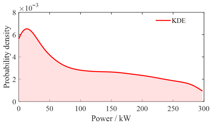
This paper selects the measured distributed wind power output data from a region in China for the year 2023 as the research object, with a sampling interval of 1 h. The probability density distribution obtained through the KDE based on this data is shown in Figure 1.

In Figure 1, it can be observed that the probability density distribution of the wind power output samples does not follow the traditional normal distribution characteristics. Specifically, it does not present a symmetric bell-shaped curve centered around the mean, but instead exhibits a pronounced right-skewed characteristic. More specifically, the samples show a higher probability density in the low power range of [0, 50] kW. As the power increases, the probability density gradually decreases and extends into a longer tail, reflecting the overall asymmetry and long-tail characteristics of the distribution.

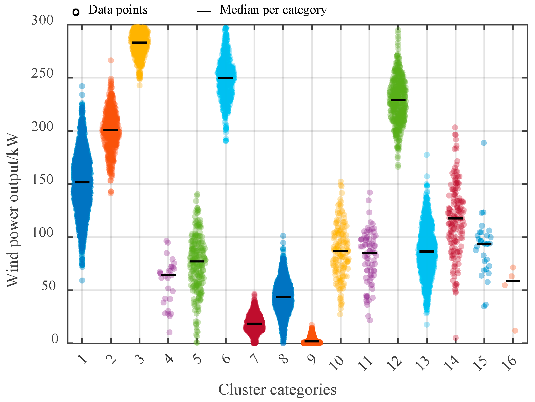
The wind power output samples are further clustered by using the DPMM. After 200 iterations, the clustering results are shown in Figure 2.

As can be seen from Figure 2, the wind power output samples are divided into 16 categories after clustering by the DPMM. Clear differences are observed among different categories in terms of output range and distribution pattern. For example, Category 9 is concentrated within a relatively narrow power interval, and its median is located around 0 kW. By contrast, Categories 1, 5, and 6 cover wider ranges. In addition, since the sample size of Category 16 is only 4, the data are insufficient to support reliable probability distribution fitting. Therefore, this category is excluded from the subsequent analysis.

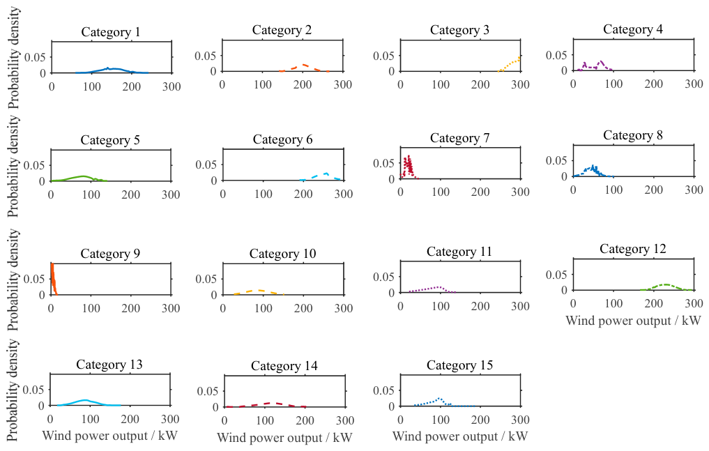
The probability density functions of wind power output samples in the 15 categories are fitted separately by using the adaptive non-parametric KDE method, and the optimal bandwidth of samples in each category is determined. The fitting results are shown in Figure 3.

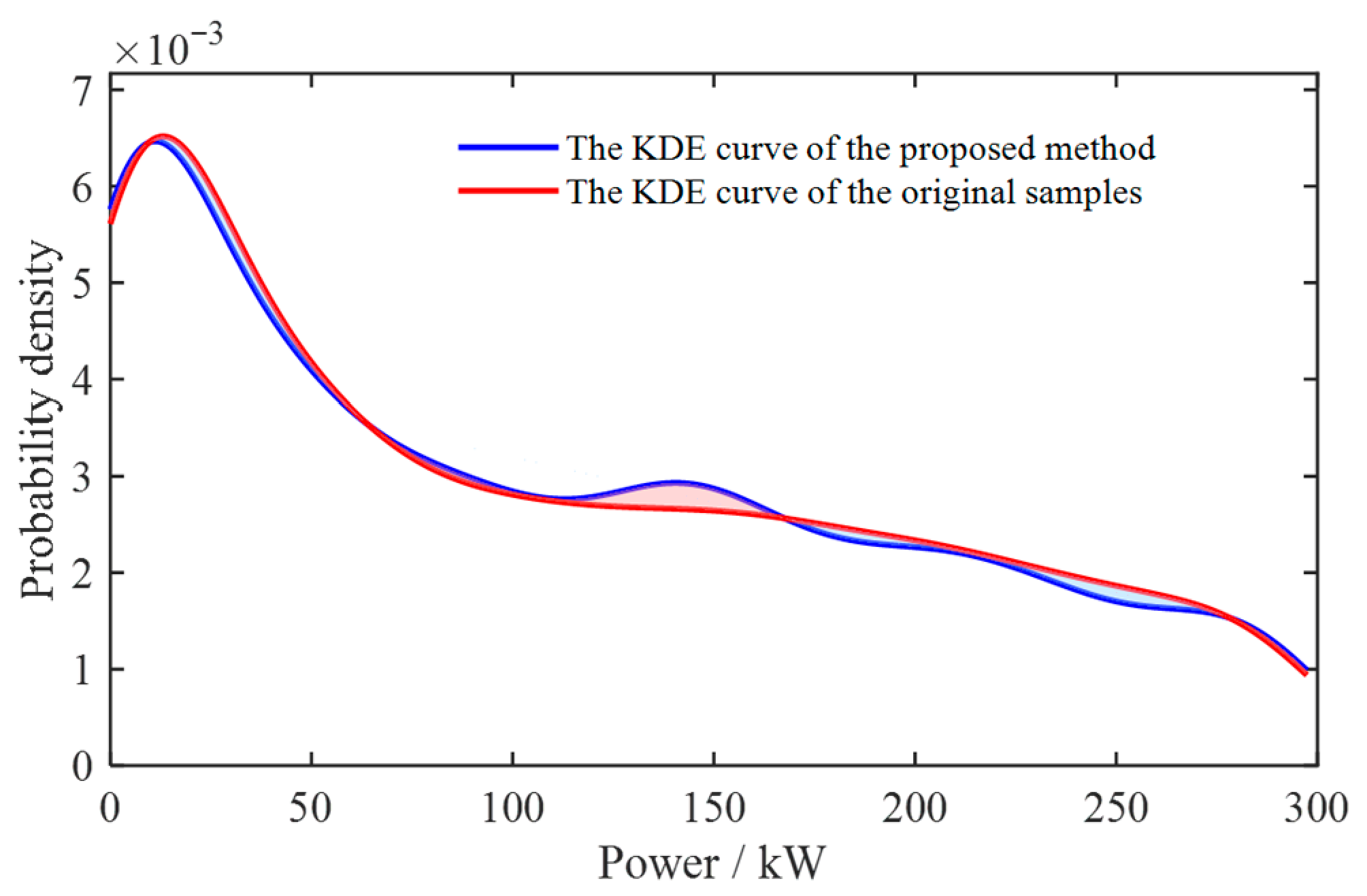
Based on the PDFs constructed with the optimal bandwidth of each category, 20,000 samples are separately drawn from the probability density function of each category by using the LHS method. A sample data distribution based on DPMM clustering is thus finally constructed. A comparison between the probability density curve of this distribution and the KDE result of the original samples is shown in Figure 4.

The results in Figure 4 indicate that the sample probability density curve generated by the proposed method remains highly consistent with the original samples in terms of overall shape. However, clear advantages are exhibited in the characterization of local distribution features. In particular, within the power interval from 110 to 270 kW, the KDE curve of the original samples shows a relatively smooth trend. By contrast, the curve obtained by the proposed method exhibits stronger capability in capturing local features within this interval, and the potential structural characteristics of the data distribution are reflected more accurately. It can therefore be seen that, while overall distribution consistency is maintained, the local features in the medium and high power interval are represented more accurately by the proposed method. This demonstrates its effectiveness in probability distribution characterization.

3.2. Analysis of Probabilistic Power Flow Results in a Distribution Network

In this section, three cases are set for probabilistic power flow calculation in the distribution network. Case 1 is the probabilistic power flow calculation method based on Monte Carlo simulation, in which the number of Monte Carlo simulation (MCS) samples is set to 10,000. Case 2 is the probabilistic power flow calculation method based on non-parametric KDE. Case 3 is the probabilistic power flow calculation method based on the DPMM and the adaptive KDE method.

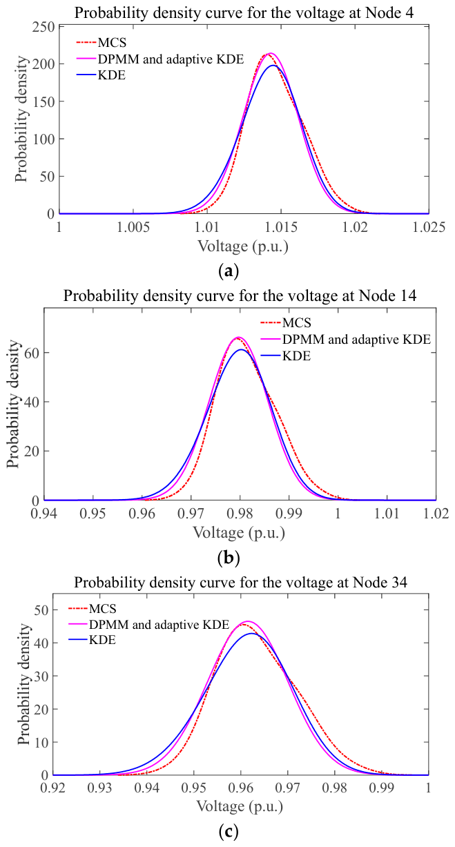
Nodes 4, 14, and 34 are selected as the objects of analysis. The results of different cases for the voltage magnitudes of these nodes are shown in Figure 5.

As can be seen from Figure 5, when the MCS results are taken as the benchmark, the probabilistic power flow method proposed in this paper, which is based on the DPMM and adaptive KDE, produces voltage magnitude distributions at Nodes 4, 14, and 34 that are closer to the MCS results than those obtained by the probabilistic power flow method based on KDE. This indicates that the probabilistic power flow method based on the DPMM and adaptive KDE can effectively ensure the calculation accuracy of the probability density curves of voltage magnitude.

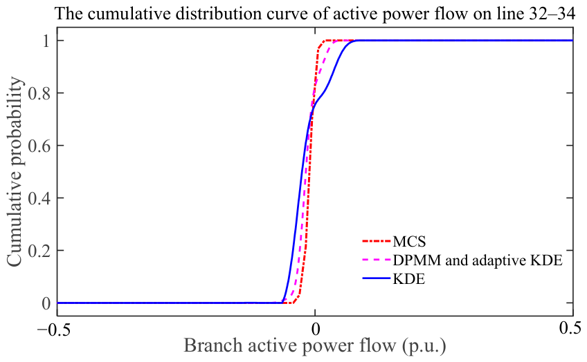
Line 32 to 34 is selected as the object of analysis. The results of different cases for the cumulative probability of active power flow on this line are shown in Figure 6. In Figure 6, the line power flow curve obtained by the probabilistic power flow method based on the DPMM and adaptive KDE is closer to the MCS result than that obtained by the KDE method.

Under the same computer configuration, the probabilistic power flow of the distribution network is calculated and compared using both the DPMM and adaptive KDE-based method and the traditional MCS method. The results show that the calculation time of the MCS method is 54.26 s, while the DPMM and adaptive KDE-based method only requires 14.86 s, improving the computational efficiency by approximately 3.6 times. Meanwhile, the probability distributions of node voltage and branch power flow obtained by the DPMM and adaptive KDE-based method are close to those from the MCS. In summary, the proposed method significantly reduces the computational cost while maintaining accuracy, ensuring the effectiveness of the distribution network risk assessment results.

In addition, to further evaluate the computational efficiency of the proposed method for a larger-scale system, the IEEE 118-bus system is also tested under the same computer configuration. The results show that the calculation time of the CM and Gram–Charlie method is 612.84 s, whereas the MCS method requires 2635.22 s. Although the computation times of both methods increase with system size, the CM and Gram–Charlie method remains faster because probabilistic characteristics are obtained through sensitivity-based cumulant propagation and distribution reconstruction, rather than through repeated full power flow calculations for a large number of random samples.

3.3. Analysis of the Validity of Risk Indices

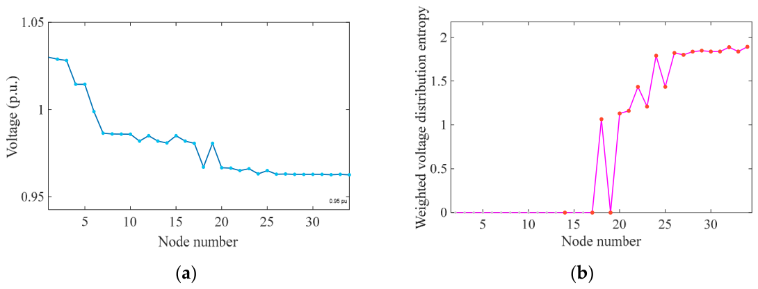
To study the effectiveness of the index based on distribution entropy theory, this section compares deterministic risk assessment with the weighted voltage distribution entropy and weighted power flow distribution entropy indices. The calculation results of the weighted voltage distribution entropy are shown in Figure 7.

In Figure 7, randomness in load and renewable energy output is not considered in the deterministic evaluation. Rather, power flow calculation is performed after the injected power at system nodes is averaged. As can be seen from Figure 7a, under the deterministic evaluation, the voltages of all nodes remain within the qualified interval from 0.95 to 1.05 p.u., and no limit violation is observed. However, when randomness is introduced and the weighted voltage distribution entropy is calculated, the results in Figure 7b show that voltage limit violation risk exists at Node 14 and Nodes 17 to 34, involving a total of 10 nodes. It can therefore be seen that, if the fluctuations of load and renewable energy are ignored, the potential risk of the distribution network is underestimated by the deterministic evaluation, and the actual risk state of the system cannot be truly reflected.

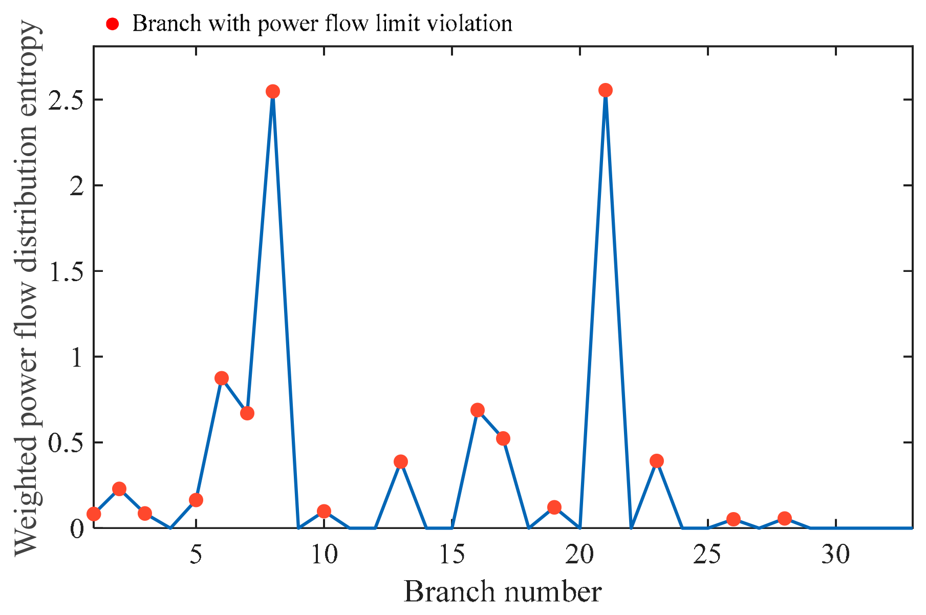
In addition, the calculated results of the power flow limit violation index are shown in Figure 8.

As can be seen from Figure 8, 16 branches are exposed to power flow limit violation risk, namely, Branches 1, 2, 3, 5, 6, 7, 8, 10, 13, 16, 17, 19, 21, 23, 26, and 28. Among these branches, Branches 6, 7, 8, 16, 17, and 21 exhibit more pronounced risk. This indicates larger power flow fluctuations, which may be associated with load variations and the instability of renewable energy output. Higher weighted power flow distribution entropy values are also observed on these branches, indicating a higher frequency of power flow exceeding the prescribed limits and a greater potential threat to grid stability. By contrast, although limit violation risk is also observed on the remaining branches, the severity remains relatively low and the risk is controllable.

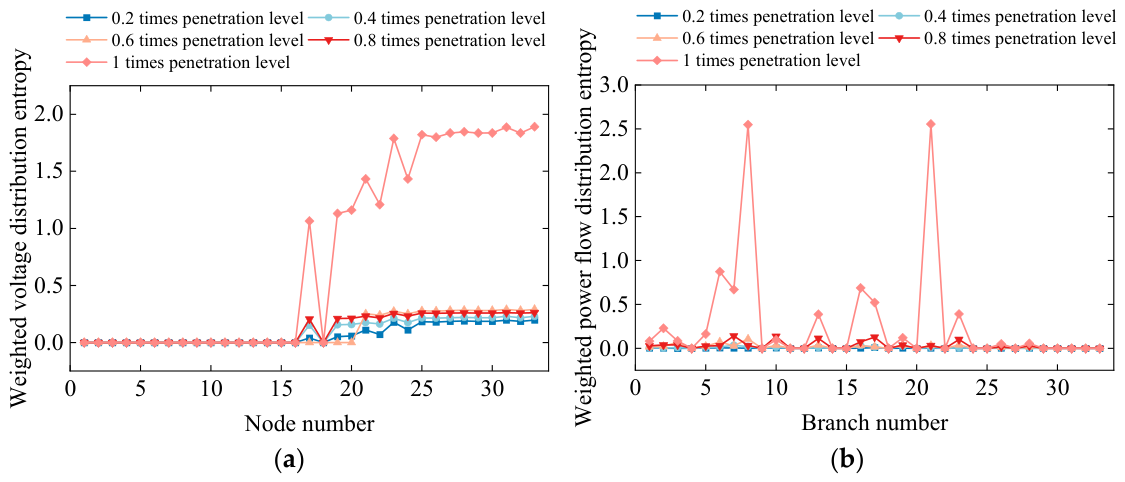
3.4. Risk Assessment Under Different Wind Power Penetration Levels

To analyze the influence of different wind power penetration levels on the risk of the distribution network, wind power penetration levels are set in this paper at 0.2, 0.4, 0.6, 0.8, and 1 times the wind power output data obtained by the DPMM and adaptive KDE method. The calculated results of weighted voltage distribution entropy and weighted power flow distribution entropy for all nodes and branches are shown in Figure 9.

As can be seen from Figure 9, significant differences are observed in the weighted voltage distribution entropy and weighted power flow distribution entropy of nodes and branches under different wind power penetration levels. In Figure 9a, regardless of the wind power penetration level, Nodes 2 to 16 are located far from the wind power node. The influence of wind power fluctuations on the system is therefore weak, and the distribution entropy values remain close to zero. The risk of voltage limit violations at these nodes can thus be regarded as negligible. As the penetration level increases, wind power fluctuations are gradually transmitted through the network. The voltages of buses close to the wind power node are more strongly affected, and both volatility and uncertainty increase significantly. When the penetration level reaches 1 times, a pronounced increase in distribution entropy is observed at several buses near the wind power node. This indicates that voltage randomness is enhanced and the risk of limit violations is aggravated at these nodes.

In Figure 9b, the weighted power flow distribution entropy of branches changes relatively smoothly when the penetration level ranges from 0.2 to 0.8 times. This indicates that line power flow fluctuations remain relatively controllable under low and medium penetration levels. However, when the penetration level increases to 1 times, the power flow distribution entropy of several critical branches rises sharply. In particular, Branches 8 and 21 exhibit evident entropy peaks, indicating that the power flow fluctuations borne by these two lines are the largest under high wind power penetration, and that the risk of limit violations is the most prominent. This is mainly because large wind power fluctuations are transmitted through adjacent branches, causing frequent changes in both power flow direction and magnitude, and significantly reducing the power flow security margin under high penetration operation.

In summary, as the wind power penetration level increases, both voltage and power flow fluctuations in the system are significantly intensified. The resulting risk exhibits concentrated and regional characteristics, which are particularly evident near the wind power integration point and adjacent branches.

In addition, since Equations (14) and (15) are based on a first-order linearization, an additional error assessment is carried out under the wind penetration level of 1.0 in order to evaluate the linearization error under the high-penetration condition. Bus 31 voltage and Branch 21 power flow are selected as representative variables, and the results obtained by the proposed method are compared with those from MCS. The compared indicators include the 95% quantile, the violation probability, and the relative error. The calculation methods for each index are as follows:

(i)

The 95% quantile

For a random variable X, the 95% quantile, denoted by Q_0.95(X), is defined as follows:

$$F_X\left(Q_{0.95}\left(X\right)\right)=0.95$$

(32)

where F_X(⋅) is the cumulative distribution function of X.

Therefore,

$$F_{V_{31}}\left(Q_{0.95}\left(V_{31}\right)\right)=0.95$$

(33)

$$F_{P_{\mathrm{line} 21–22}}\left(Q_{0.95}\left(P_{\mathrm{line} 21–22}\right)\right)=0.95$$

(34)

In the proposed method, the corresponding CDF is obtained from Equation (23) together with Equations (25) and (26). In the MCS method, the 95% quantile is extracted directly from the ordered samples.

(ii)

Violation probability

For the V₃₁, if the undervoltage risk is considered, the violation probability is defined as follows:

$$P_{\mathrm{vio}}\left(V_{31}\right)=P\left(V_{31}<V_{\min }\right)+P\left(V_{31}>V_{\max }\right)$$

(35)

For the P_{line 21–22}, the violation probability is defined as follows:

$$P_{\mathrm{vio}}\left(P_{\mathrm{line} 21–22}\right)=P\left(P_{\mathrm{line} 21–22}>P_{\max }\right)$$

(36)

$$P_{\max }=k\cdot \left|P_{\mathrm{line} 21–22}^0\right|$$

(37)

where $P_{\mathrm{line} 21–22}^0$ is the base-case active power flow; k is a preset margin coefficient.

In the MCS method, the violation probability is obtained from the sample frequency.

(iii)

Relative error

For any compared index X, the relative error is defined as follows:

$${\epsilon }_X={\displaystyle \frac{\left|X_{\mathrm{MCS}}-X_{\mathrm{CM}–\mathrm{GC}}\right|}{\left|X_{\mathrm{CM}–\mathrm{GC}}\right|}}\times 100\%$$

(38)

The results are shown in

Table 1. Calculated results for each indicator.

Variable	Indicator	CM and Gram–Charlier	MCS	Relative Error (%)
V31	95% quantile	0.9770	0.9756	0.1434
V31	Violation probability	0.7880	0.7879	0.0124
Pline 21–22	95% quantile	0.4230	0.3547	16.1371
Pline 21–22	Violation probability	0.0599	0	100

.

As shown in Table 1, good agreement is maintained for the 95% quantile and the violation probability of Bus 31 voltage V₃₁, which indicates that the proposed method still provides satisfactory accuracy for the voltage-related probabilistic indices at this bus. In contrast, the discrepancy becomes more evident for the tail-related indices of Branch 21 power flow $P_{\mathrm{line} 21–22}$. The relative error of its 95% quantile reaches 16.1371%, and a larger difference is also observed in the violation probability. This indicates that, under the high wind penetration condition, the first-order linearization becomes less effective in capturing branch-flow tail behavior, which is consistent with the increased linearization error near the operating limit.

4. Conclusions

In this paper, an uncertainty risk assessment method applicable to distribution network is proposed on the basis of the DPMM and CM. The effectiveness and feasibility of the proposed method are verified through case analysis. The main conclusions are given as follows.

(1)

The DPMM is employed in this paper to cluster wind power output data, and the bandwidth parameter of each category for wind power data is calculated on the basis of the adaptive non-parametric KDE method. Local features of wind power output data can be effectively captured by this method. In particular, in the medium and high power intervals, the fitting accuracy of the data is improved through adaptive bandwidth adjustment.

(2)

Considering the uncertainty of wind power and load, a probabilistic power flow model for distribution networks is proposed on the basis of CM and the Gram–Charlier series expansion. Compared with the KDE model, the proposed method can approximate the MCS results more accurately in the probability distributions of system state variables. In addition, compared with the MCS, the proposed method improves computational efficiency to a certain extent while ensuring calculation accuracy.

(3)

A weighted distribution entropy index is designed to quantify the risk impact of wind power and load uncertainty on voltage and power in the distribution network. Through comparative analysis under different wind power penetration levels, it is shown that the risk in system voltage and power distributions increases with wind power penetration. In particular, under high penetration conditions, the limit violation risk of some branches and nodes rises significantly, which further confirms the potential threat of uncertainty to distribution network security.

(4)

The proposed uncertainty risk assessment method enables the identification of high-risk nodes, high-risk branches, and high-risk periods in distribution networks, thereby providing support for real-time dispatch and preventive control. In addition, the proposed weighted distribution entropy index can be incorporated as a risk warning quantity, a dispatch-trigger signal, or a risk term in optimization.

References

1. Gruosso, G.; Gajani, G.S.; Maffezzoni, P. Nonlinear Power Injection Sensitivity Analysis in Power Systems: An Effective Strategy for Distributed Source Allocation. IEEE Trans. Circuits Syst. I Regul. Pap. 2025, 73, 696–706. [Google Scholar] [CrossRef]
2. Li, J.; He, M.; Huang, S.D.; Wu, X.; Fan, L.; Liu, Z.Y. Ground fault protection algorithm of active distribution network based on energy extremum direction. IET Gener. Transm. Distrib. 2024, 18, 4279–4290. [Google Scholar] [CrossRef]
3. Etanya, T.F.; Tsafack, P.; Ngwashi, D.K. Grid-connected distributed renewable energy generation systems: Power quality issues, and mitigation techniques—A review. Energy Rep. 2025, 13, 3181–3203. [Google Scholar] [CrossRef]
4. Li, Y.M.; Wang, J.J.; Cao, Y.H. Multi-objective distributed robust cooperative optimization model of multiple integrated energy systems considering uncertainty of renewable energy and participation of electric vehicles. Sustain. Cities Soc. 2024, 104, 105308. [Google Scholar] [CrossRef]
5. Chen, X.P.; Wang, L.; Jiang, Y.N.; Wang, J.X. A peer-to-peer joint energy and reserve market considering renewable generation uncertainty: A generalized Nash equilibrium approach. Energy Convers. Econ. 2024, 5, 179–192. [Google Scholar] [CrossRef]
6. Gandhi, O.; Kumar, D.S.; Rodríguez-Gallegos, C.D.; Srinivasan, D. Review of power system impacts at high PV penetration Part I: Factors limiting PV penetration. Sol. Energy 2020, 210, 181–201. [Google Scholar] [CrossRef]
7. Pan, L.R.; Yang, X.; Yuan, S.B.; Li, J.A.; Xue, H.W. Risk Assessment of New Distribution Network Dispatching Operations Considering Multiple Uncertain Factors. Electronics 2025, 14, 4012. [Google Scholar] [CrossRef]
8. Wang, H.; Sui, L.F.; Bian, J.; Yu, H.N.; Li, G.Q. Integrated operation risk assessment of distribution network based on improved subjective and objective combination weighting and ISODATA. Electr. Power Syst. Res. 2024, 233, 110469. [Google Scholar] [CrossRef]
9. Chen, L.J.; Liu, L.; Peng, Y.; Chen, W.J.; Huang, H.Y.; Wu, T.T.; Xu, X.H. Distribution network operational risk assessment and early warning considering multi-risk factors. IET Gener. Transm. Distrib. 2020, 14, 136–154. [Google Scholar] [CrossRef]
10. Lei, J.Z.; Gong, Q.W.; Gao, D.W.Z.; Wang, B.H.; Guan, X.Y. Operation risk assessment of active distribution networks considering probabilistic uncertainties of distributed generators-loads and power management of VRB ESSs. IET Renew. Power Gener. 2020, 14, 1764–1771. [Google Scholar] [CrossRef]
11. Yu, J.F.; Li, Q.Q.; Du, Y.; Wang, R.T.; Li, R.F.; Guo, D.B. Voltage over-limit risk assessment of wind power and photovoltaic access distribution system based on day-night segmentation and Gaussian mixture model. Energy Rep. 2024, 12, 2812–2823. [Google Scholar] [CrossRef]
12. Clavijo-Blanco, J.A.; González-Cagigal, M.A.; Rosendo-Macías, J.A. Statistical characterization of reliability indices in medium voltage networks using a Monte Carlo-based method. Electr. Power Syst. Res. 2024, 234, 110585. [Google Scholar] [CrossRef]
13. Morales, J.M.; Perez-Ruiz, J. Point estimate schemes to solve the probabilistic power flow. IEEE Trans. Power Syst. 2007, 22, 1594–1601. [Google Scholar] [CrossRef]
14. Verbic, G.; Canizares, C.A. Probabilistic optimal power flow in electricity markets based on a two-point estimate method. IEEE Trans. Power Syst. 2006, 21, 1883–1893. [Google Scholar] [CrossRef]
15. Fan, M.; Vittal, V.; Heydt, G.T.; Ayyanar, R. Probabilistic power flow studies for transmission systems with photovoltaic generation using cumulants. IEEE Trans. Power Syst. 2012, 27, 2251–2261. [Google Scholar] [CrossRef]
16. Huang, J.W.; Du, Z.Y.; Cai, H.W.; He, J.X.; Yue, G.H.; Li, G.; Zhao, H.; Chen, Y. Probabilistic load flow calculation and power system security analysis based on improved CGC-CM. Electr. Power Syst. Res. 2024, 237, 110995. [Google Scholar] [CrossRef]
17. Hu, W.; Yang, F.; Shen, Y.; Yang, Z.C.; Chen, H.C.; Lei, Y. Dynamic risk assessment of voltage violation in distribution networks with distributed generation. Entropy 2023, 25, 1662. [Google Scholar] [CrossRef]
18. Liu, S.; Ma, Y.M.; Pan, Y.T.; Zhao, W.C.; Gao, Q.Z.; Guan, X.K. Risk assessment of photovoltaic system based on cumulant method and mixed copula. Electr. Eng. 2025, 107, 5137–5148. [Google Scholar] [CrossRef]
19. Luo, Y.H.; Wang, X.; Yan, S.J. Risk assessment of photovoltaic distribution network based on adaptive kernel density estimation and cumulant method. Energy Rep. 2022, 8, 1152–1159. [Google Scholar] [CrossRef]
20. Cai, W.C.; Gao, Y.; Zhang, X.P.; Si, Q.; Jia, J.X.; Li, B.Z. Safety Assessment of Loop Closing in Active Distribution Networks Based on Probabilistic Power Flow. Energies 2025, 18, 2685. [Google Scholar] [CrossRef]
21. Chen, X.L.; Han, J.; Zheng, T.T.; Zhang, P.; Duan, S.M.; Miao, S.H. A vine-copula based voltage state assessment with wind power integration. Energies 2019, 12, 2019. [Google Scholar] [CrossRef]
22. Seguro, J.V.; Lambert, T.W. Modern estimation of the parameters of the Weibull wind speed distribution for wind energy analysis. J. Wind Eng. Ind. Aerodyn. 2000, 85, 75–84. [Google Scholar] [CrossRef]
23. Chang, T.P. Performance comparison of six numerical methods in estimating Weibull parameters for wind energy application. Appl. Energy 2011, 88, 272–282. [Google Scholar] [CrossRef]
24. Khan, M.G.M.; Ahmed, M.R. Bayesian method for estimating Weibull parameters for wind resource assessment in a tropical region: A comparison between two-parameter and three-parameter Weibull distributions. Wind Energy Sci. 2023, 8, 1277–1298. [Google Scholar] [CrossRef]
25. Fernandez-Jimenez, L.A.; Monteiro, C.; Ramirez-Rosado, I.J. Short-term probabilistic forecasting models using Beta distributions for photovoltaic plants. Energy Rep. 2023, 9, 495–502. [Google Scholar] [CrossRef]
26. Hu, B.; Li, Y.D.; Yang, H.J.; Wang, H. Wind speed model based on kernel density estimation and its application in reliability assessment of generating systems. J. Mod. Power Syst. Clean Energy 2017, 5, 220–227. [Google Scholar] [CrossRef]
27. Wang, S.; Sun, Y.H.; Zhang, W.J.; Srinivasan, D. Optimization of deterministic and probabilistic forecasting for wind power based on ensemble learning. Energy 2025, 319, 134884. [Google Scholar] [CrossRef]
28. Zhang, K.; Yu, X.D.; Liu, S.L.; Dong, X.; Li, D.Q.; Zang, H.Z.; Xu, R. Wind power interval prediction based on hybrid semi-cloud model and nonparametric kernel density estimation. Energy Rep. 2022, 8, 1068–1078. [Google Scholar] [CrossRef]
29. Gu, B.; Shen, H.Q.; Lei, X.H.; Hu, H.; Liu, X.Y. Forecasting and uncertainty analysis of day-ahead photovoltaic power using a novel forecasting method. Appl. Energy 2021, 299, 117291. [Google Scholar] [CrossRef]
30. Wu, Z.X.; Lin, S.F.; Tan, J.; Li, D.D. Multi-scenario stochastic assessment of operational risk of integrated energy system based on R-vine Copula. Electr. Power Syst. Res. 2025, 245, 111569. [Google Scholar] [CrossRef]
31. Lin, S.F.; Liu, C.T.; Shen, Y.W.; Li, F.X.; Li, D.D.; Fu, Y. Stochastic planning of integrated energy system via frank-copula function and scenario reduction. IEEE Trans. Smart Grid 2021, 13, 202–212. [Google Scholar] [CrossRef]
32. Yang, N.; Huang, Y.; Hou, D.X.; Liu, S.K.; Ye, D.; Dong, B.T.; Fan, Y.P. Adaptive nonparametric kernel density estimation approach for joint probability density function modeling of multiple wind farms. Energies 2019, 12, 1356. [Google Scholar] [CrossRef]
33. Li, L.Y.; Li, Z.B. A Hybrid Interval prediction framework for photovoltaic power prediction using BiLSTM—transformer and adaptive kernel density estimation. Appl. Sci. 2026, 16, 3023. [Google Scholar] [CrossRef]
34. Gao, Y.H.; Xu, X.Y.; Yan, Z.; Shahidehpour, M. Gaussian mixture model for multivariate wind power based on kernel density estimation and component number reduction. IEEE Trans. Sustain. Energy 2022, 13, 1853–1856. [Google Scholar] [CrossRef]
35. Zhang, X.X.; Dong, G.W.; Shi, J.; Zhang, Y.N.; Wang, Y.M.; Xu, R.J.; Chen, K.; Suslov, K.; Gu, B.; Ma, Y. Configuration Optimization of Hybrid Energy Storage System Based on Dynamic Weighted Power Prediction Error Distribution. IEEE Trans. Ind. Appl. 2025, 61, 7836–7846. [Google Scholar] [CrossRef]
36. Abramson, I.S. On bandwidth variation in kernel estimates—A square root law. Ann. Stat. 1982, 10, 1217–1223. [Google Scholar] [CrossRef]
37. Chau, T.T.; Nguyen, T.T.H.; Nguyen, L.; Ton, D.D. Wind speed probability distribution based on adaptive bandwidth kernel density Estimation model for wind farm application. Wind Energy 2025, 28, e2970. [Google Scholar] [CrossRef]
38. Zhang, Y.; Wang, C.; Hu, X. An adaptive importance sampling method based on improved MCMC simulation for structural reliability analysis. Appl. Sci. 2025, 15, 10438. [Google Scholar] [CrossRef]
39. Zhang, P.; Lee, S.T. Probabilistic load flow computation using the method of combined cumulants and Gram-Charlier expansion. IEEE Trans. Power Syst. 2004, 19, 676–682. [Google Scholar] [CrossRef]
40. Yang, J.X.; Yi, Y.Q.; Zhang, Y.J.; Mo, Y.F.; Huang, T.C.; Xie, X.Y. Operation risk analysis of elec-tric vehicle integrated to distribution network based on weighted distribution entropy. Autom. Electr. Power Syst. 2020, 44, 171–179. [Google Scholar]
Figure 1. Probability density of wind power output samples.
Inventions 11 00042 g001
Figure 2. Clustering results of the DPMM.
Inventions 11 00042 g002
Figure 3. Probability density distributions of various wind power samples.
Inventions 11 00042 g003
Figure 4. Comparison of probability density curves between original samples and samples from the proposed method.
Inventions 11 00042 g004
Figure 5. Node voltage probability density curve. (a) Probability density curve for the voltage at Node 4; (b) Probability density curve for the voltage at Node 14; (c) Probability density curve for the voltage at Node 34.
Inventions 11 00042 g005
Figure 6. Active power cumulative distribution for line l32–34.
Inventions 11 00042 g006
Figure 7. Voltage assessment results. (a) Nodal voltages by the deterministic evaluation method; (b) Nodal voltages by the weighted voltage distribution entropy method.
Inventions 11 00042 g007
Figure 8. Calculation results of weighted power flow distribution entropy.
Inventions 11 00042 g008
Figure 9. Weighted voltage and power flow distribution entropy under different penetration levels. (a) Weighted voltage distribution entropy under different penetration levels; (b) Weighted power flow distribution entropy under different penetration levels.
Inventions 11 00042 g009