Systematic Characterisation and Non-Linear Response Correction of SiPMs Using the Single-Step Method for High-Precision Calorimetry

Abstract

Silicon photomultipliers (SiPMs) are vital for calorimetric applications in high-energy physics and medical imaging due to their high gain, compactness, and insensitivity to magnetic fields. However, their finite pixel count induces non-linear response behaviour at high photon fluxes, affecting energy resolution and systematic accuracy. This work presents a comprehensive methodology to characterise SiPM response functions and derive correction curves using a single-step laser-based measurement approach. Three SiPMs with varying pixel sizes (15, 25 and 50 µm) are studied under controlled temperature conditions, with response functions extracted across different overvoltages and integration windows. The correction method, independent of precise light source calibration, effectively linearises the response up to saturation levels exceeding 100% of the pixel count, achieving deviations of the order of 3% across a broad operational parameter space, and outperforming the traditional calibration model. The analysis demonstrates minimal dependence of the correction on temperature, overvoltage, and pixel size, indicating universal applicability. These findings enhance SiPM performance in high-energy calorimetry and offer a practical framework for improving detector linearity and dynamic range extensions in large-scale applications.

1. Introduction

Silicon photomultipliers (SiPMs) are extensively applied in high-energy physics calorimeters for detecting scintillation light due to their high gain, compact size, and magnetic field immunity. Key applications include large-scale hadron calorimeters (HCALs) in CMS [1], high-granularity imaging calorimeters (CALICEs) [2], sampling calorimeters (SpaCals) [3], and future collider detectors (EICs) [4] to measure particle energy and shower shape. SiPMs are also widely used in Positron Emission Tomography (PET) calorimeters to detect gamma-ray scintillation [5].

SiPM’s non-linear response, a consequence of the finite number of pixels operated in Geiger mode, causes significant signal saturation at high photon rates, degrading calorimetric energy resolution and inducing systematic energy biases. Non-linearity reduces the measured signal below linear predictions, particularly in high-energy showers, requiring precise correction to recover energy linearity. As SiPMs reach saturation, the response becomes non-linear (onset typically already at 15% of pixels fired), thereby degrading the resolution at high energies. Ultimately, the limited number of pixels limits the maximum measurable energy (the detector’s dynamic range) before saturation occurs.

This effect is most relevant for calorimeters for high-energy particle detectors, but also for the measurements of $\mathrm{keV}$ photons in PET/SPECT detectors [6]. In [7], for example, the non-linearity of energy response for each channel of a PET detector is calibrated using multiple radioactive sources. Ref. [8] demonstrates how the channel-to-channel calibration of SiPM non-linear response is obtained and successfully applied to improve energy resolution for $511 \mathrm{keV}$ photons in a PET system. In these examples, channel-by-channel calibration of the non-linear response is performed on the assembled detector at its operating conditions, using known energy sources as references. This method is usually not applicable to highly granular calorimeters, where hundreds of thousands of channels must be calibrated. In addition, the detector may need to be operated under different temperature and voltage conditions during its lifetime, e.g., to compensate for the effects of radiation damage.

Non-linearity can be corrected by characterising the response curve against a known variable light source. The measurement of saturation effects in SiPMs with a light source and their phenomenological parametrisation have been discussed in detail in the literature, e.g., in [9,10]. In [11], SiPMs with 100, 400, 1600, and 2668 pixels with sub-nanosecond light pulses of different intensities were investigated; in [12], SiPMs were exposed to light pulses of different intensities and pulse lengths; and, in [13], saturation effects of a SiPM using UV light were investigated. Related approaches based on light superposition have also been proposed, e.g., in [14]. More measurements presented in the literature are summarised in [15,16]. The application of these correction curves assumes that they are independent of SiPM operation parameters, or that the dependence can be calibrated away. Additionally, it assumes that the illumination scheme used during calibration is the same as during data taking. The single-step approach differs from direct response-curve calibrations because it derives the correction function without requiring an absolute calibration of the light-intensity axis. In our study, we intend to critically analyse all these assumptions and factorise the various effects into separate parametrisations.

The simplest parametrisation of the SiPM response curve is given by [17]:

$$N_{\mathrm{fired}}=N_{\mathrm{pix}}·\left(1-e^{-{\displaystyle \frac{N_{\gamma }·\mathit{PDE}}{N_{\mathrm{pix}}}}}\right),$$

(1)

with $N_{\gamma }$ the number of incident photons, $N_{\mathrm{fired}}$ the number of fired pixels, and $N_{\mathrm{pix}}$ the number of pixels in the SiPM. The number of fired pixels is usually calculated in units of photoelectrons, removing the gain dependence of the SiPM response. This compensates for part of the temperature and voltage dependence of the response function, but the dependence of the photo-detection efficiency, $\mathit{PDE}(\mathit{V},\mathit{T})$, remains.

Our approach is to separate the understanding of the SiPM response function into two steps: the response function for instantaneous and homogeneous light distribution, and the response function considering the time and spatial distribution of light. In this work, we focus on the first step, the determination and systematic study of the response function to instantaneous and homogeneous light. The aim is to extract a correction function independent of the calibration of the light source and study its dependence on SiPM operation (temperature, voltage, and integration gate length) and design parameters (pixel capacitance). This paper completes and extends the study presented in [18] by reporting measurements with a modified and improved experimental setup, including SiPMs with different pixel sizes, and providing a systematic evaluation of the correction method as a function of overvoltage, temperature, and integration gate length.

The paper is organised as follows: Section 2 presents the setup for the non-linearity measurements of SiPMs based on the single-step method presented in [19]. This delivers a correction function that is independent of the light source calibration. In Section 3, three SiPMs with different pixel capacitances are characterised, and the response function is measured. This provides a generalised correction function for the experiment utilising these SiPMs. In Section 4, we study how the response function varies as a function of the operating parameters, and how the correction function extracted in Section 3 in laboratory conditions performs to linearise the response in these experimental conditions. In Section 5, the conclusions of the study are presented.

2. Materials and Methods

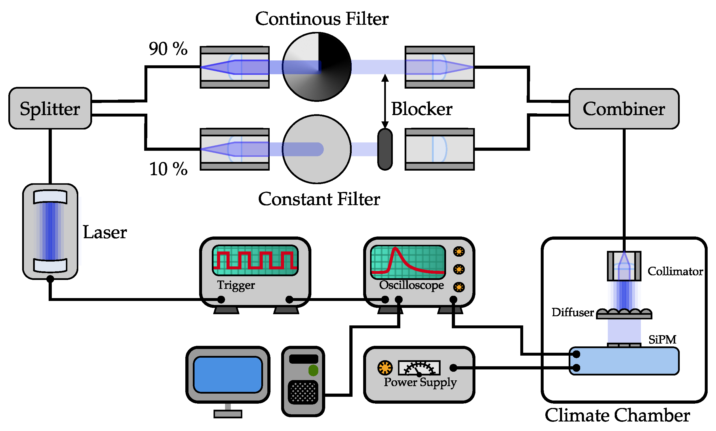
In this study, three $1.2\times 1.2$ mm² SiPM samples from KETEK [20] are characterised. Their pixel sizes are 15, 25 and 50 μm, corresponding, respectively, to the pixel capacitances $C_{\mathrm{pix}}$ of 8.7, 22.7 and 111.5 fF calculated with Equation (3). All other relevant properties are listed in

Table 1. Key parameters of the SiPMs used in this paper. The parameters were extracted from the gain scan described in Section 3.1. All SiPMs were produced by KETEK [20] and have a sensitive area of $1.2\times 1.2 {\mathrm{mm}}^2$.

SiPM Type	PM1150	PM1125	PM1115
Pixel size [$\mathrm{\mu }\mathrm{m}$]	50	25	15
Number of pixels, $N_{\mathrm{pix}}$	576	2304	4832
Gain × ${10}^5$ @ $\Delta V=5 \mathrm{V}$, $T=20 °\mathrm{C}$	34.8 ± 0.1	7.09 ± 0.02	2.73 ± 0.02
Pixel capacitance, $C_{\mathrm{pix}}$ [fF]	111.5 ± 0.4	22.72 ± 0.06	8.73 ± 0.06
Turn-off voltage [$\mathrm{V}$] @ $T=20 °\mathrm{C}$	27.58 ± 0.01	27.45 ± 0.01	26.66 ± 0.02
Temperature coefficient [$\mathrm{m}\mathrm{V} {\mathrm{K}}^{-1}$]	21.4 ± 0.2	20.9 ± 0.4	26.7 ± 0.7
Afterpulse probability @ $\Delta V=5 \mathrm{V}$ [%]	71	6.8 ± 0.4	2.6 ± 0.7
Crosstalk probability @ $\Delta V=5 \mathrm{V}$ [%]	7.2 ± 0.6	6.9 ± 0.4	7.2 ± 0.8

. During the preparation of this work, the setup described in [18] was upgraded. We verified that measurements taken with the upgraded configuration are consistent with those obtained with the original setup, and the results presented here include data from both. A sketch of the new setup is shown in Figure 1. The main change is the transition from two independent light sources to a single one. This ensures that the illumination schemes used in the single-step method, described in Section 2, share the same temporal profile, as they originate from the same laser source. The light source is a picosecond pulsed laser with a pulse width of $t_{\mathrm{P}}=50$ ps and a wavelength of ${\lambda }_{\mathrm{Laser}}=451$ nm. The laser pulse width is negligible compared to the recovery time of the three SiPM samples (on the order of tens of nanoseconds). The laser light is split using an optical splitter fibre into a main branch containing $90\%$ of the intensity and a minor branch containing 10%. The main branch provides a base pulse of variable intensity that can be adjusted across four orders of magnitude via a continuous optical neutral-density wheel. The minor branch provides a constant additional light intensity, set by fixed neutral-density filters. A mechanical light blocker is used to selectively block either one branch or to leave both branches unblocked. The two branches are then coupled into a single fibre combiner to illuminate the SiPM. The fibre output is shaped by an optical diffuser, providing a spatially uniform illumination of the SiPM. The sample is mounted inside a climate chamber on a micrometric stage to ensure stable and controlled temperature and humidity conditions during data taking. Further details on the setup calibration are given in [19,21]. The SiPM signal is read out with an oscilloscope, and the integrated pulse current from each waveform is stored on a computer for further analysis.

The main parameters relevant to this study are measured and monitored as follows:

• Temperature (T) and humidity inside the climate chamber are recorded via a DKRF4002 temperature humidity sensor [22], close to the SiPM. After each temperature adjustment, the system is allowed to thermalise for approximately one hour. Thermal stability is considered reached when the SiPM current stabilises and the temperature of the climate chamber T is taken as equal to the SiPM temperature.
• The SiPM overvoltage $\Delta V=V_{\mathrm{bias}}-V_{\mathrm{off}}$, is defined as the difference between the applied bias voltage and the turn-off voltage. The turn-off voltage is determined for every temperature with the procedure explained in Section 3.1.
• The SiPM gain (G) is the charge generated by the detection of a single photon in one pixel divided by the elementary charge $q_0$. It is a function of the operating conditions and the integration gate, $G(T,V_{\mathrm{bias}},t_{\mathrm{g}})$. The gain can be approximated with the capacitance of the pixels as [23]:

  $$G={\displaystyle \frac{1}{q_0}}\left(C_{\mathrm{pix}}\left(V_{\mathrm{bias}}\right)V_{\mathrm{bias}}-C_{\mathrm{pix}}(V_{\mathrm{off}}\right)V_{\mathrm{off}}).$$

  (2)
  If the pixel capacitance $C_{\mathrm{pix}}$ does not change for $V_{\mathrm{bias}}\ge V_{\mathrm{off}}$, Equation (2) simplifies to

  $$G={\displaystyle \frac{C_{\mathrm{pix}}(V_{\mathrm{bias}}-V_{\mathrm{off}})}{q_0}}.$$

  (3)
  Since G can be directly measured from charge spectra at low light intensity (Section 3.1), Equation (3) can be inverted to determine $C_{\mathrm{pix}}$.
• The signal integration gate ($t_{\mathrm{g}}$) is the window duration in which the recorded waveform is integrated. The gate starting time is adjusted to $5 \mathrm{n}\mathrm{s}$ before the rising edge of the signal. Integration gate lengths of $400 \mathrm{n}\mathrm{s}$ ($50 \mathrm{\mu }\mathrm{m}$), $120 \mathrm{n}\mathrm{s}$ ($25 \mathrm{\mu }\mathrm{m}$) and $200 \mathrm{n}\mathrm{s}$ ($15 \mathrm{\mu }\mathrm{m}$) were selected to include at least $95\%$ of the total charge while avoiding additional noise. For the $15 \mathrm{\mu }\mathrm{m}$ pitch SiPM, the gain measurements were performed with an AMP-0611 amplifier from Photonique SiPM [24]. The amplifier introduces a small time delay and a minor change in the pulse shape. With short integration gates, this could lead to different fractions of the signal being integrated with and without the amplifier. To ensure this effect is negligible, a gate length of $200 \mathrm{n}\mathrm{s}$ was chosen for this device, to integrate the full pulse in both cases. The amplification factor was determined from dedicated measurements with the $25 \mathrm{\mu }\mathrm{m}$ SiPM, for which the gain can be measured with and without the amplifier, and was found to be $A_{\mathrm{amplifier}}=46.73\pm 0.26$.

Single-Step Method

A method first introduced by Gatti and Piva in 1953 [25] to overcome the problems of differential non-linearity in pulse height encoding was later described by Wright [26] for the measurement of the non-linearity of photomultiplier tubes (PMTs). The so-called single-step method can be used to measure the non-linearity in DC and pulsed signals in PMTs. This section presents the concept of this method adapted to the present setup; additional details are explained in [18]. The single-step method allows for determining the non-linearity of the SiPM response by measuring the change in its output when a small, constant-intensity light pulse is added to a base pulse of variable intensity. The advantage of this method is that it does not require an absolute calibration of the base-light source, and the correction function is completely determined from the measured responses of the SiPM. The measured quantity is the charge, with the possibility of using the pulse height as an alternative.

The base-light pulse, with variable intensity $I_i$ spans the full dynamic range of the SiPM, with the number of impinging seed photons $N_{\mathrm{seed}}$ ranging from zero to exceeding the number of pixels of the SiPM $N_{\mathrm{pix}}$. The number of seed photons is the number of photons triggering a Geiger avalanche in the absence of saturation and it is defined as the number of impinging photons ($N_{\gamma }$) on the SiPM times the photo-detection efficiency ($\mathit{PDE}$):

$$N_{\mathrm{seed}}=N_{\gamma }·\mathit{PDE}.$$

(4)

The additional light pulse is provided by the second light source, ideally matched in wavelength and pulse length. The intensity of the additional light is set to be sufficient to produce a measurable difference at low intensity, while remaining within the SiPM’s linear regime. Typical values are between $3\%$ and $5\%$ of $N_{\mathrm{pix}}$.

In the setup of Figure 1, the base pulse is delivered by the $90\%$ branch and its intensity is scanned with the neutral-density wheel, while the additional pulse is provided by the $10\%$ branch and kept constant with fixed attenuation. Therefore, each step of the method corresponds to a specific angle of the neutral-density wheel. For each step, the mean charge of the SiPM is measured twice: first as the response to the base light only ($\mu \left(1^{\mathrm{st}}\right)$), and second as the response to the base light plus the additional light ($\mathit{\mu }\left(2^{\mathrm{nd}}\right)$). The local differential response of the SiPM to the constant additional light pulse (i.e., the local slope of the response curve) can be approximated with:

$$S\left(\mathit{\mu }\right)={\displaystyle \frac{\mathit{\mu }\left(2^{\mathrm{nd}}\right)-\mathit{\mu }\left(1^{\mathrm{st}}\right)}{{\mathit{\mu }}^{*}}},$$

(5)

where ${\mathit{\mu }}^{*}$ is the measured mean charge when the SiPM is illuminated by the additional light pulse only. Each step is associated with a single operating point by defining $\mathit{\mu }$ as the mean of the two measured charges:

$$\mathit{\mu }={\displaystyle \frac{1}{2}}\left(\mathit{\mu }\left(1^{\mathrm{st}}\right)+\mathit{\mu }\left(2^{\mathrm{nd}}\right)\right).$$

(6)

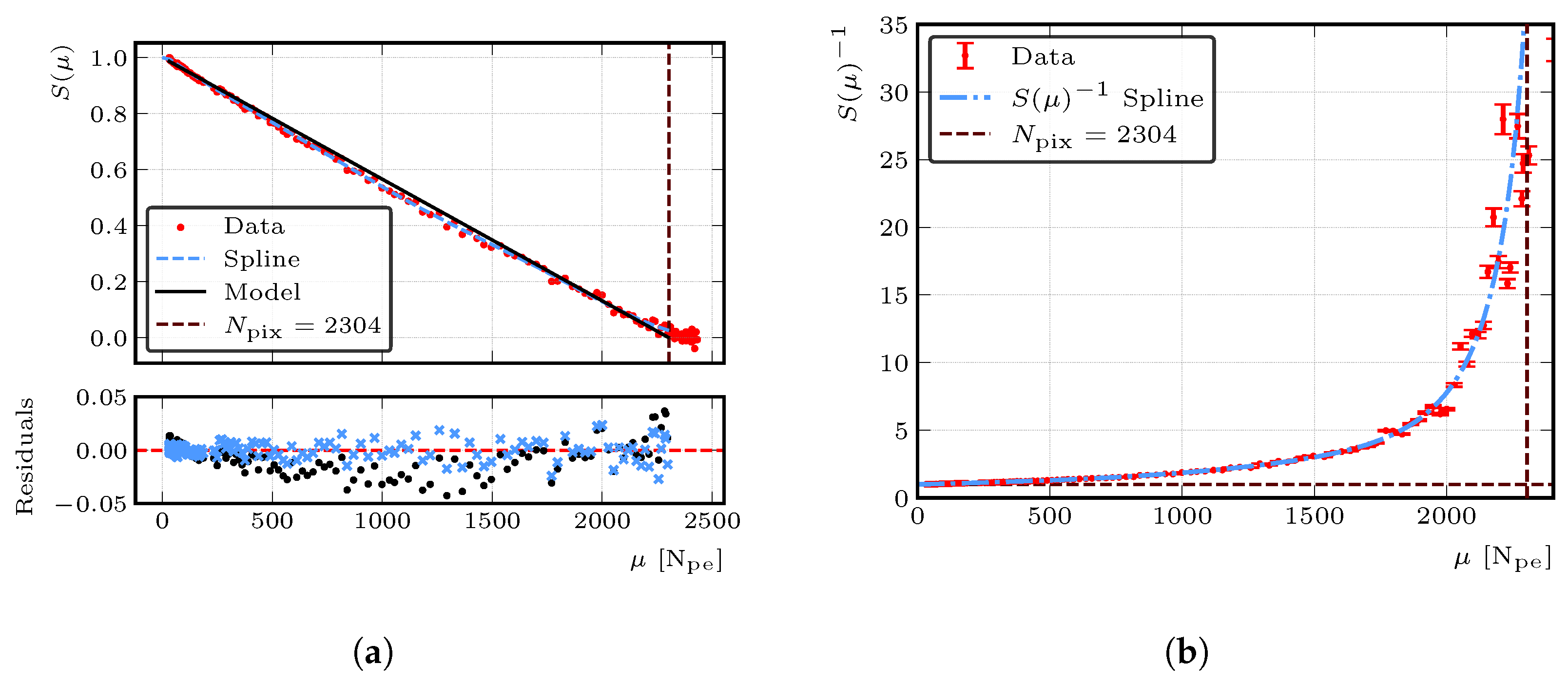
Figure 2a shows the measured slope $S\left(\mathit{\mu }\right)$ for the $25 \mathrm{\mu }\mathrm{m}$ SiPM as a function of $\mathit{\mu }$. In the linear regime, the additional light pulse is fully detected and the numerator in Equation (5) is approximately ${\mathit{\mu }}^{*}$; therefore, $S\left(\mathit{\mu }\right)\approx 1$.

Table 2. Range and step size of the scan parameters used in a measurement cycle. The end value for the gate length dependence is $200 \mathrm{n}\mathrm{s}$ for the $15 \mathrm{\mu }\mathrm{m}$ pixel pitch SiPM, $120 \mathrm{n}\mathrm{s}$ for the $25 \mathrm{\mu }\mathrm{m}$ pixel pitch SiPM and $400 \mathrm{n}\mathrm{s}$ for the $50 \mathrm{\mu }\mathrm{m}$ pixel pitch SiPM.

Scan Parameter	Starting Value	End Value	Step	Reference Value
				15 μm	25 μm	50 μm
Temperature, T [$°\mathrm{C}$]	20	−20	5	20	20	20
Overvoltage, $\Delta V$ [$\mathrm{V}$]	3	5	0.5	5	5	5
Gate length, $t_{\mathrm{g}}$ [$\mathrm{n}\mathrm{s}$]	10	see Ref.	10	200	120	400

Table 2. Range and step size of the scan parameters used in a measurement cycle. The end value for the gate length dependence is $200 \mathrm{n}\mathrm{s}$ for the $15 \mathrm{\mu }\mathrm{m}$ pixel pitch SiPM, $120 \mathrm{n}\mathrm{s}$ for the $25 \mathrm{\mu }\mathrm{m}$ pixel pitch SiPM and $400 \mathrm{n}\mathrm{s}$ for the $50 \mathrm{\mu }\mathrm{m}$ pixel pitch SiPM.

Scan Parameter	Starting Value	End Value	Step	Reference Value
				15 μm	25 μm	50 μm
Temperature, T [$°\mathrm{C}$]	20	−20	5	20	20	20
Overvoltage, $\Delta V$ [$\mathrm{V}$]	3	5	0.5	5	5	5
Gate length, $t_{\mathrm{g}}$ [$\mathrm{n}\mathrm{s}$]	10	see Ref.	10	200	120	400

As the base-light intensity increases, the detected fraction of the additional light decreases, and so does $S\left(\mathit{\mu }\right)$. In the saturation limit, no further additional light can be detected and $S\left(\mathit{\mu }\right)$ approaches zero. From the exponential model in Equation (1), the expected dependence of $S\left(\mathit{\mu }\right)$ on $\mathit{\mu }$ is linear:

$$S\left(\mathit{\mu }\right)=1-{\displaystyle \frac{\mathit{\mu }}{N_{\mathrm{pix}}}}.$$

(7)

This expectation is shown by the black line in Figure 2a. The residual plot at the bottom, defined as the difference between the data and the spline or model expectation, indicates that Equation (7) does not fully describe the data, as it systematically overestimates $S\left(\mathit{\mu }\right)$. Instead, to better reproduce the measured trend, a smoothing third-order B-spline is applied to the $S\left(\mathit{\mu }\right)$ vs. $\mathit{\mu }$ data (dashed blue line). Since $S\left(\mathit{\mu }\right)$ is the local derivative of the response curve, its reciprocal $S{\left(\mathit{\mu }\right)}^{-1}$ represents the local correction factor needed to restore linearity [26], and is evaluated for both the data and the spline. The result is shown in Figure 2b. For an ideal linear device, $S{\left(\mathit{\mu }\right)}^{-1}=1$ over the full range (dashed horizontal line). Deviations from 1 quantify the onset of saturation and non-linearity, especially as $\mathit{\mu }$ approaches $N_{\mathrm{pix}}$. The correction can then be applied to any measured charge $\mathit{\mu }$ by evaluating the following integral:

$${\mathit{\mu }}_{\mathrm{corr}}={\int }_0^{\mathit{\mu }}S{\left({\mathit{\mu }}^{\prime }\right)}^{-1}\mathrm{d}{\mathit{\mu }}^{\prime }.$$

(8)

The additional area between the constant value 1 and the spline accounts for the non-linearity of the SiPM. This correction operates directly on the measured charge of each individual event without any assumption on the ensemble mean, making it naturally applicable on an event-by-event basis. This is a key advantage over the analytical correction from Equation (1), which is derived from Poisson statistics and, by construction, gives the expectation value of the number of fired pixels over an ensemble of events; applying it to recover the number of incident photons from a single charge measurement implicitly requires the measured charge to equal the ensemble mean, which only holds when averaging over many events. Finally, we define the correction factor $f_{\mathrm{corr}}$ as the ratio between the corrected and the measured charge:

$$f_{\mathrm{corr}}={\displaystyle \frac{{\mathit{\mu }}_{\mathrm{corr}}}{\mathit{\mu }}},$$

(9)

where ${\mathit{\mu }}_{\mathrm{corr}}$ is obtained from Equation (8).

3. Measurements

For each SiPM, two types of measurement are performed. First, dedicated gain scans are performed under low light intensity to characterise the gain dependence on temperature (T), bias voltage ($V_{\mathrm{bias}}$), and integration gate length ($t_{\mathrm{g}}$) for each SiPM. The resulting dependencies, $\frac{\mathsf{\partial }G}{\mathsf{\partial }{V}_{\mathrm{bias}}}$, $\frac{\mathrm{d}{V}_{\mathrm{off}}}{\mathrm{d}T}$, and $\frac{\mathsf{\partial }G}{\mathsf{\partial }{t}_{\mathrm{g}}}$, are parametrised by fit functions and applied either analytically or on a point-by-point basis in subsequent analyses. The turn-off voltage at each temperature is extracted from the gain-vs-voltage fits and used to define the bias settings for the following light-intensity scans.

In the second step, light-intensity scans are performed across a matrix of temperature and overvoltage values. For each acquisition of N events, the waveforms recorded with the oscilloscope are processed online during the measurement. Storing the full waveforms for every event would require substantial disk space; instead the pulse current is integrated, and only the resulting charge is stored. The integration is performed in $10 \mathrm{n}\mathrm{s}$ intervals, which allows the charge to be reconstructed offline for arbitrary gate lengths that are multiples of $10 \mathrm{n}\mathrm{s}$. This approach greatly reduces the data volume while retaining enough timing information for offline studies, without the need to repeat measurements. The chosen reference operating conditions for which the correction function is obtained are $T_{\mathrm{ref}}=20 °\mathrm{C}$, overvoltage $\Delta V_{\mathrm{ref}}=5 \mathrm{V}$, and integration gate lengths reported in Table 2.

3.1. Gain Scans

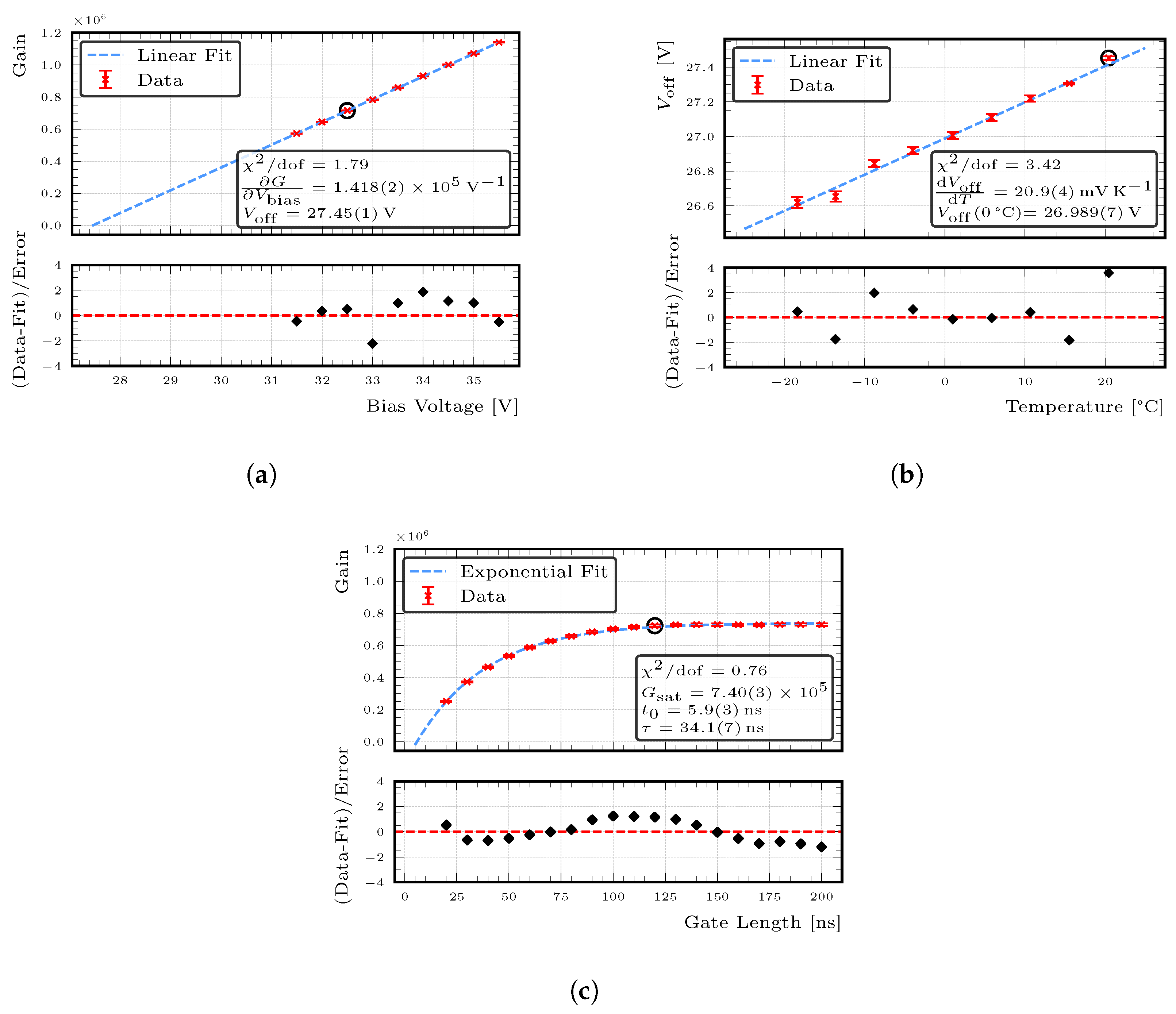
The gain scan consists of a sequence of measurements in which the SiPM is illuminated with only a few photons for different bias voltages and temperatures. The charge spectra are analysed using the PeakOTron [27] Python module, which fits a dedicated SiPM detector response model to extract the gain as the distance between adjacent photoelectron peaks, along with other relevant SiPM parameters. The key quantities extracted from this measurement are the gain dependence on the bias voltage $\frac{\mathsf{\partial }G}{\mathsf{\partial }{V}_{\mathrm{bias}}}$, the turn-off voltage dependence on the temperature $\frac{\mathrm{d}{V}_{\mathrm{off}}}{\mathrm{d}T}$ and the gain dependence on the integration gate length $\frac{\mathsf{\partial }G}{\mathsf{\partial }{t}_{\mathrm{g}}}$. Figure 3 presents the result of the gain scan for the $25 \mathrm{\mu }\mathrm{m}$ pixel pitch SiPM starting from the reference operating condition and varying one parameter at a time.

Table 3. Parameters of the fit functions to the gain dependence on bias voltage, the turn-off voltage dependence on the temperature and the gain dependence on the integration gate length for the three investigated SiPMs.

Function	$\mathit{G}=\frac{\mathsf{\partial }\mathit{G}}{{\mathsf{\partial }\mathit{V}}_{\mathbf{bias}}}({\mathit{V}}_{\mathbf{bias}}-{\mathit{V}}_{\mathbf{off}})$		${\mathit{V}}_{\mathbf{off}}=\left(\frac{\mathbf{d}{\mathit{V}}_{\mathbf{off}}}{\mathbf{d}\mathit{T}}\right)\mathit{·}\mathit{T}+{\mathit{V}}_{\mathbf{off}}\left(0 °\mathbf{C}\right)$		$\mathit{G}={\mathit{G}}_{\mathbf{sat}}\left(1-exp\left(-\frac{\mathit{t}-{\mathit{t}}_0}{\mathit{\tau }}\right)\right)$
Parameters	$\frac{\mathsf{\partial }\mathit{G}}{\mathsf{\partial }{\mathit{V}}_{\mathbf{bias}}}\times {\mathbf{10}}^{\mathbf{5}}$ $[{\mathbf{V}}^{\mathbf{-}\mathbf{1}}]$	${\mathit{V}}_{\mathbf{off}}$ $\mathbf{[}\mathbf{V}\mathbf{]}$	$\frac{\mathbf{d}{\mathit{V}}_{\mathbf{off}}}{\mathbf{d}\mathit{T}}$ $\mathbf{[}\mathbf{m}\mathbf{V} {\mathbf{K}}^{\mathbf{-}\mathbf{1}}\mathbf{]}$	${\mathit{V}}_{\mathbf{off}}\mathbf{\left(}\mathbf{0} \mathbf{°}\mathbf{C}\mathbf{\right)}$ $\mathbf{[}\mathbf{V}\mathbf{]}$	${\mathit{G}}_{\mathbf{sat}}\mathbf{\times }{\mathbf{10}}^{\mathbf{5}}$	${\mathit{t}}_{\mathbf{0}}$ $\mathbf{[}\mathbf{n}\mathbf{s}\mathbf{]}$	$\mathit{\tau }$ $\mathbf{[}\mathbf{n}\mathbf{s}\mathbf{]}$
PM1115	$0.545\pm 0.003$	$26.66\pm 0.02$	$26.7\pm 0.7$	$26.110\pm 0.010$	$4.084\pm 0.004$	$4.82\pm 0.02$	$18.4\pm 0.1$
PM1125	$1.418\pm 0.002$	$27.45\pm 0.01$	$20.9\pm 0.4$	$26.989\pm 0.007$	$7.400\pm 0.028$	$5.92\pm 0.34$	$34.1\pm 0.7$
PM1150	$6.955\pm 0.024$	$27.58\pm 0.01$	$21.4\pm 0.2$	$27.151\pm 0.003$	$36.485\pm 0.058$	$2.35\pm 0.11$	$126.2\pm 0.6$

Table 3. Parameters of the fit functions to the gain dependence on bias voltage, the turn-off voltage dependence on the temperature and the gain dependence on the integration gate length for the three investigated SiPMs.

Function	$\mathit{G}=\frac{\mathsf{\partial }\mathit{G}}{{\mathsf{\partial }\mathit{V}}_{\mathbf{bias}}}({\mathit{V}}_{\mathbf{bias}}-{\mathit{V}}_{\mathbf{off}})$		${\mathit{V}}_{\mathbf{off}}=\left(\frac{\mathbf{d}{\mathit{V}}_{\mathbf{off}}}{\mathbf{d}\mathit{T}}\right)\mathit{·}\mathit{T}+{\mathit{V}}_{\mathbf{off}}\left(0 °\mathbf{C}\right)$		$\mathit{G}={\mathit{G}}_{\mathbf{sat}}\left(1-exp\left(-\frac{\mathit{t}-{\mathit{t}}_0}{\mathit{\tau }}\right)\right)$
Parameters	$\frac{\mathsf{\partial }\mathit{G}}{\mathsf{\partial }{\mathit{V}}_{\mathbf{bias}}}\times {\mathbf{10}}^{\mathbf{5}}$ $[{\mathbf{V}}^{\mathbf{-}\mathbf{1}}]$	${\mathit{V}}_{\mathbf{off}}$ $\mathbf{[}\mathbf{V}\mathbf{]}$	$\frac{\mathbf{d}{\mathit{V}}_{\mathbf{off}}}{\mathbf{d}\mathit{T}}$ $\mathbf{[}\mathbf{m}\mathbf{V} {\mathbf{K}}^{\mathbf{-}\mathbf{1}}\mathbf{]}$	${\mathit{V}}_{\mathbf{off}}\mathbf{\left(}\mathbf{0} \mathbf{°}\mathbf{C}\mathbf{\right)}$ $\mathbf{[}\mathbf{V}\mathbf{]}$	${\mathit{G}}_{\mathbf{sat}}\mathbf{\times }{\mathbf{10}}^{\mathbf{5}}$	${\mathit{t}}_{\mathbf{0}}$ $\mathbf{[}\mathbf{n}\mathbf{s}\mathbf{]}$	$\mathit{\tau }$ $\mathbf{[}\mathbf{n}\mathbf{s}\mathbf{]}$
PM1115	$0.545\pm 0.003$	$26.66\pm 0.02$	$26.7\pm 0.7$	$26.110\pm 0.010$	$4.084\pm 0.004$	$4.82\pm 0.02$	$18.4\pm 0.1$
PM1125	$1.418\pm 0.002$	$27.45\pm 0.01$	$20.9\pm 0.4$	$26.989\pm 0.007$	$7.400\pm 0.028$	$5.92\pm 0.34$	$34.1\pm 0.7$
PM1150	$6.955\pm 0.024$	$27.58\pm 0.01$	$21.4\pm 0.2$	$27.151\pm 0.003$	$36.485\pm 0.058$	$2.35\pm 0.11$	$126.2\pm 0.6$

The scan parameters that are not varied in each plot are fixed at their respective reference values as defined in Table 2.

First, the turn-off voltage is extracted by fitting the gain as a function of bias voltage with a linear fit function $G=\frac{\mathsf{\partial }G}{\mathsf{\partial }{V}_{\mathrm{bias}}}(V_{\mathrm{bias}}-V_{\mathrm{off}})$. This is shown in Figure 3a. The turn-off voltage $V_{\mathrm{off}}$ is defined as the voltage at which the gain is equal to 1. In this analysis, it is taken as the x-axis intercept of the linear fit. This is repeated for each temperature. Now, the dependence of the turn-off voltage on the temperature is studied. For this, a linear fit $V_{\mathrm{off}}=\left(\frac{\mathrm{d}{V}_{\mathrm{off}}}{\mathrm{d}T}\right)·T+V_{\mathrm{off}}\left(0 °\mathrm{C}\right)$ is performed, and the slope $\frac{\mathrm{d}{V}_{\mathrm{off}}}{\mathrm{d}T}$ of this function characterises the change of turn-off voltage with changing temperature as shown in Figure 3b. Finally, an appropriate gate length for each SiPM can be derived by analysing the gate length dependence of the gain. In Figure 3c the gain dependence on the gate length is fitted with the fit function $G=G_{\mathrm{sat}}\left(1-exp\left(-{\displaystyle \frac{t-t_0}{\tau }}\right)\right)$. We choose an appropriate gate length as the point where at least $95\%$ of the full gain is reached, which ensures that the majority of the signal is integrated without too much additional noise that will negatively impact the gain determination. Changing the gate length does not affect the results, as shown in Section 4.

3.2. Light-Intensity Scans

For each SiPM, two types of light-intensity scans are performed. The first scan is performed under reference conditions, following the procedure described in Section 2, and is used to determine the correction function. Each measurement consists of 50,000 events, providing an optimal trade-off between statistical precision and acquisition time.

The second scan involves varying parameters to assess the applicability of the correction function under different conditions. For this we perform a scan over temperature and overvoltage in the range of 20 °C to −20 °C in steps of $5 °\mathrm{C}$ and 3 V to 5 V in steps of $0.5 \mathrm{V}$ respectively. During this scan, only the SiPM’s response to the laser light is measured. Additionally, we reduce the number of events per point from 50,000 to 10,000 to shorten measurement time and reduce data volume.

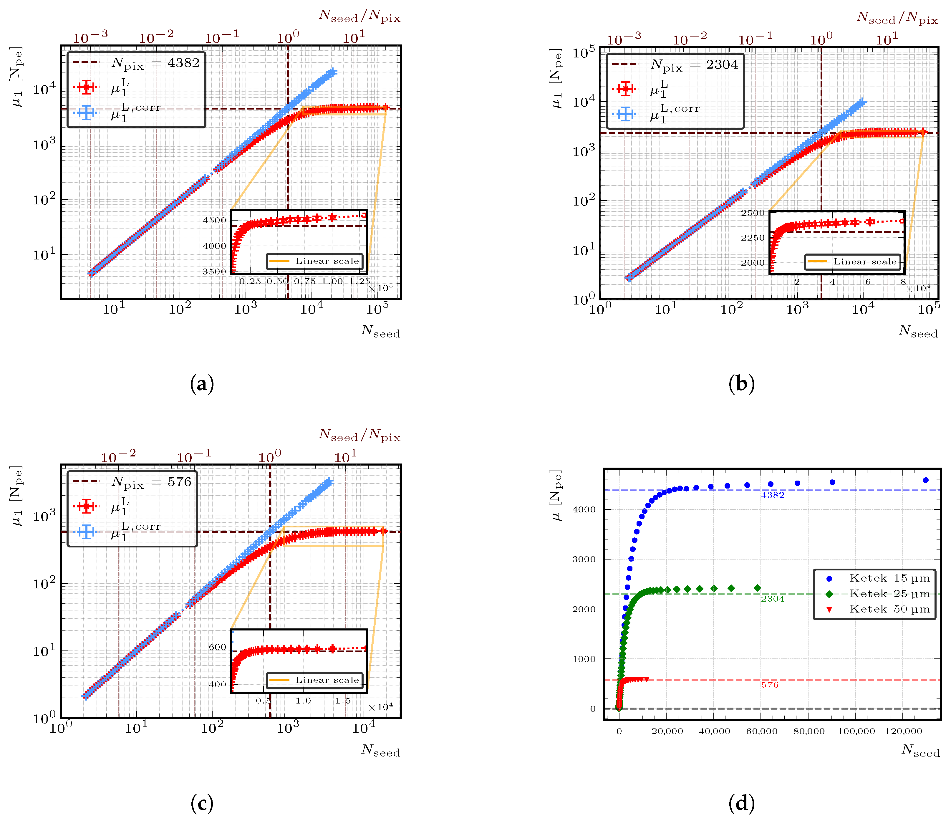
In Figure 4, the response functions of the three SiPMs with different pixel pitches, each operated under the reference conditions, are presented. The response function shows the mean of the charge, under laser light only, as a function of the number of seed photons $N_{\mathrm{seed}}$ as defined in Section 2. At low intensities, this quantity can be calibrated using the method described in [18], neglecting correlated noise. The calibration is only used for plotting and validation purposes; the correction function itself does not rely on it.

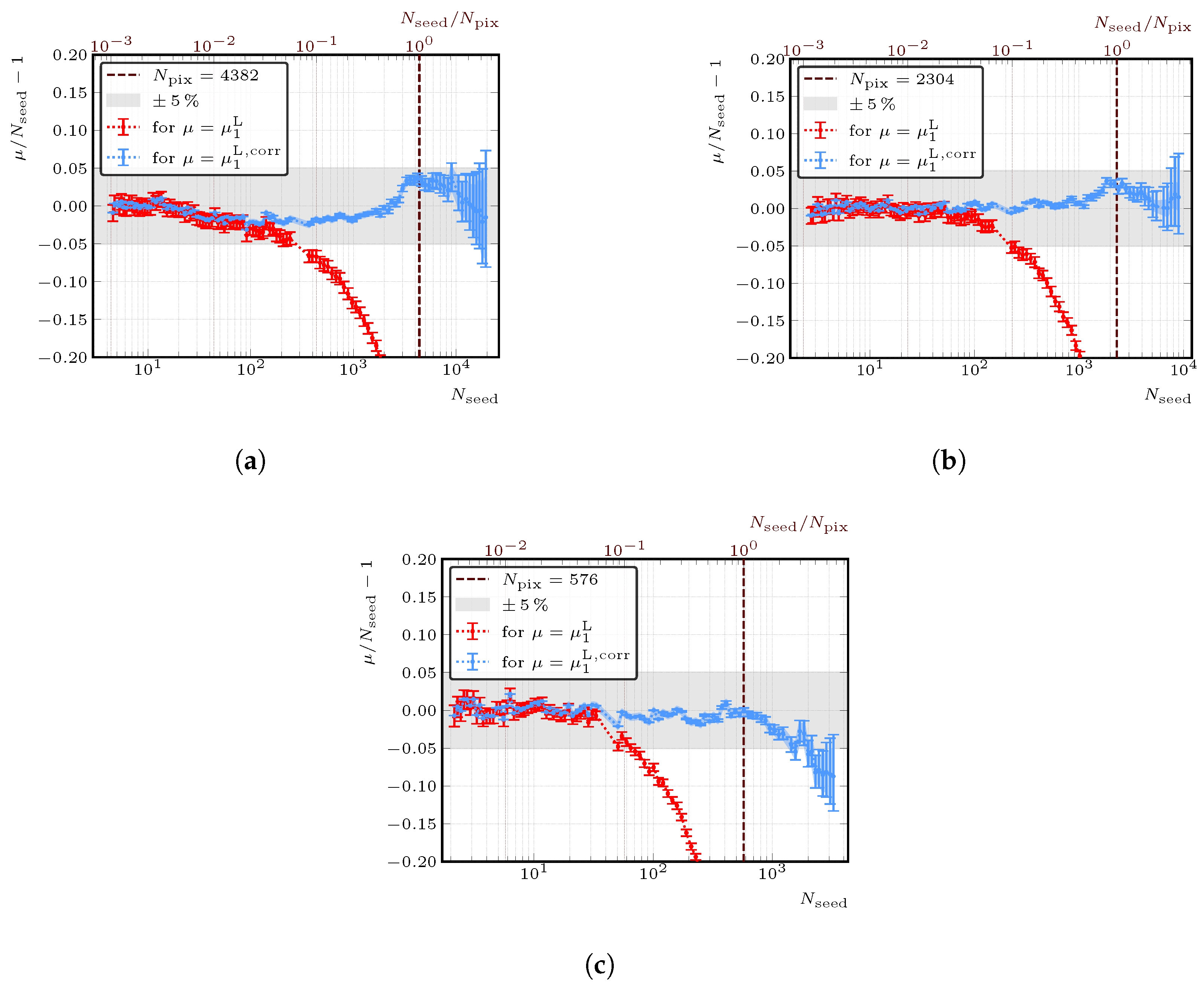
The measured SiPM response (red curve ${\mathit{\mu }}_1^{\mathrm{L}}=\mathit{\mu }\left(1^{\mathrm{st}}\right)$) is linear at low light intensities, where the number of seed photons is small compared to the number of pixels $N_{\mathrm{pix}}$ (below $5\%$ of $N_{\mathrm{pix}}$). At higher light intensities, the response becomes non-linear and approaches saturation, with a maximum signal exceeding the pixel count for all three devices: about $5\%$ above $N_{\mathrm{pix}}$ for the $15 \mathrm{\mu }\mathrm{m}$ and $25 \mathrm{\mu }\mathrm{m}$ pitch SiPMs, and $3\%$ for the $50 \mathrm{\mu }\mathrm{m}$ one. The origin of this over-saturation effect is not yet understood. The degree of over-saturation observed with our sub-nanosecond light pulse ($50 \mathrm{p}\mathrm{s}$) is smaller than what has been reported in previous studies. For example, Gruber et al. [9], found saturation levels reaching up to twice the pixel count when using short light pulses of $\approx 30 \mathrm{p}\mathrm{s}\mathrm{FWHM}$ and a Hamamatsu MPPC (S10362-11-050U), which also features a pixel size of $50 \mathrm{\mu }\mathrm{m}$.

The correction function derived from the first scan at the reference condition is then applied to the data on an event-by-event basis, with an upper bound of $\mathit{\mu }<N_{\mathrm{pix}}$ to ensure comparability across devices with different pixel counts. The corrected SiPM response (blue curve ${\mathit{\mu }}_1^{\mathrm{L},\mathrm{corr}}$) is linear over the full application range.

To evaluate the quality of correction, the deviation from a linear response is analysed and shown in Figure 5 as the percentage difference from a linear response. The percentage difference is shown on the y-axis and calculated as follows:

$${\displaystyle \frac{{\mathit{\mu }}_1}{N_{\mathrm{seed}}}}-1,$$

(10)

where either the uncorrected ${\mathit{\mu }}_1^{\mathrm{L}}$ or corrected ${\mathit{\mu }}_1^{\mathrm{L},\mathrm{corr}}$ data is used and $N_{\mathrm{seed}}$ is the number of seed photons.

A linear response corresponds to a horizontal line at zero, i.e., ${\mathit{\mu }}_{\mathrm{corr}}=N_{\mathrm{seed}}$. The corrected and uncorrected data are shown again in blue and red, respectively, for the measurements shown in Figure 4 at the reference conditions.

The three SiPMs show similar behaviour for the uncorrected data. The uncorrected response deviates by more than $5\%$ from linearity already at $N_{\mathrm{seed}}\approx 0.1N_{\mathrm{pix}}$.

For all three SiPMs, the corrected response remains within $5\%$ linearity for light intensities up to $N_{\mathrm{pix}}$. The light blue band indicates the uncertainty range of the correction function. The error bars indicate the uncertainty on the response, which is dominated by the uncertainty on the gain determination.

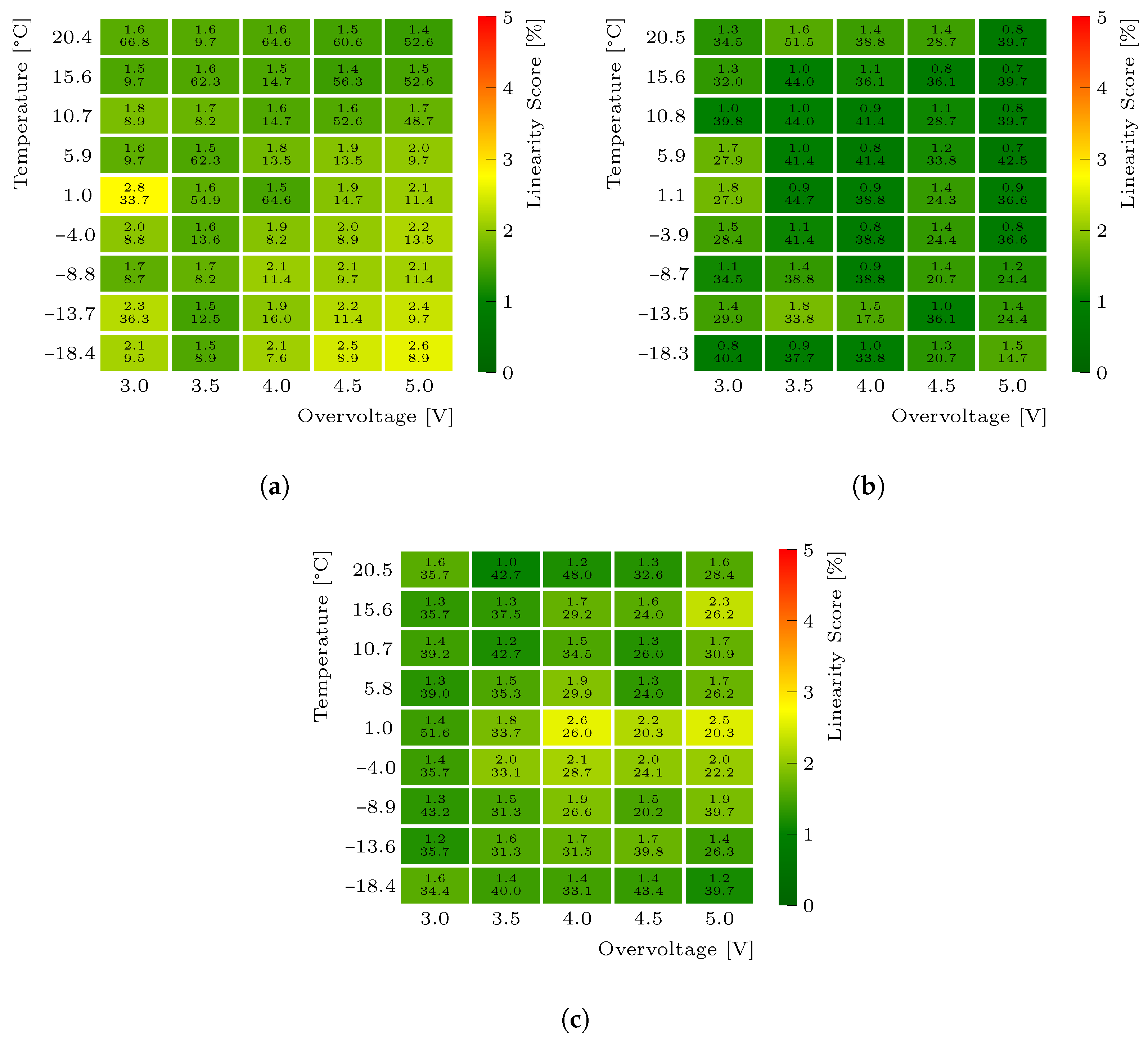
The quality of the correction is assessed based on two criteria. The first is the average absolute deviation from linearity, called the linearity score and defined as:

$$\mathcal{L}={\displaystyle \frac{{\displaystyle {\displaystyle \sum _{k=1}^{N_{\mathrm{tot}}}}\left|\frac{{\mathit{\mu }}_1^{\mathrm{L},\mathrm{corr}}}{N_{\mathrm{seed}}}-1\right|}}{N_{\mathrm{tot}}}},$$

(11)

where ${\mathit{\mu }}_1^{\mathrm{L},\mathrm{corr}}$ is the corrected response, and we sum over all measurement points $N_{\mathrm{tot}}$. The second one, called the dynamic range extension factor, is defined as:

$$\kappa ={\displaystyle \frac{N_{\mathrm{seed}}^{\mathrm{outlier},\mathrm{corr}}}{N_{\mathrm{seed}}^{\mathrm{outlier}}}},$$

(12)

$N_{\mathrm{seed}}^{\mathrm{outlier},\mathrm{corr}}$ and $N_{\mathrm{seed}}^{\mathrm{outlier}}$ are the number of seed photons at which the deviation from linearity crosses the $5\%$ level.

To verify the application range of the correction function, which was determined for the reference conditions $T=20 °\mathrm{C}$ and $\Delta V=5 \mathrm{V}$, we apply it to the measurements taken over the range of $T=-20 °\mathrm{C} \mathrm{to} 20 °\mathrm{C}$ and $\Delta V=3 \mathrm{V} \mathrm{to} 5 \mathrm{V}$. This procedure mimics a realistic application where SiPMs are first calibrated in the laboratory at room temperature and stable conditions, and then are operated inside a detector at different and possibly varying conditions.

After correction, the results are evaluated using the defined criteria, with the results summarised in the matrices shown in Figure 6.

Each cell in the matrix reports the outcome of the two metrics after applying the correction function: the linearity score (top, also represented by the colourmap) and the dynamic range extension factor (bottom).

For all three SiPMs, the correction determined at the reference conditions can be applied across the full parameter space, with no or only minor dependence on temperature and overvoltage. Figure 6b presents the $25 \mathrm{\mu }\mathrm{m}$ device as an example: the corrected response shows deviations from linearity below $2\%$ and an average dynamic range extension factor of 34 ($20-45$). Across all devices, linearity is recovered to within $3\%$ throughout the parameter space. The spread in the extension factor is mainly due to uncertainties in the gain calibration, which become significant at high intensities and dominate the variation observed at high light intensities.

4. Comparison of the Correction Factors

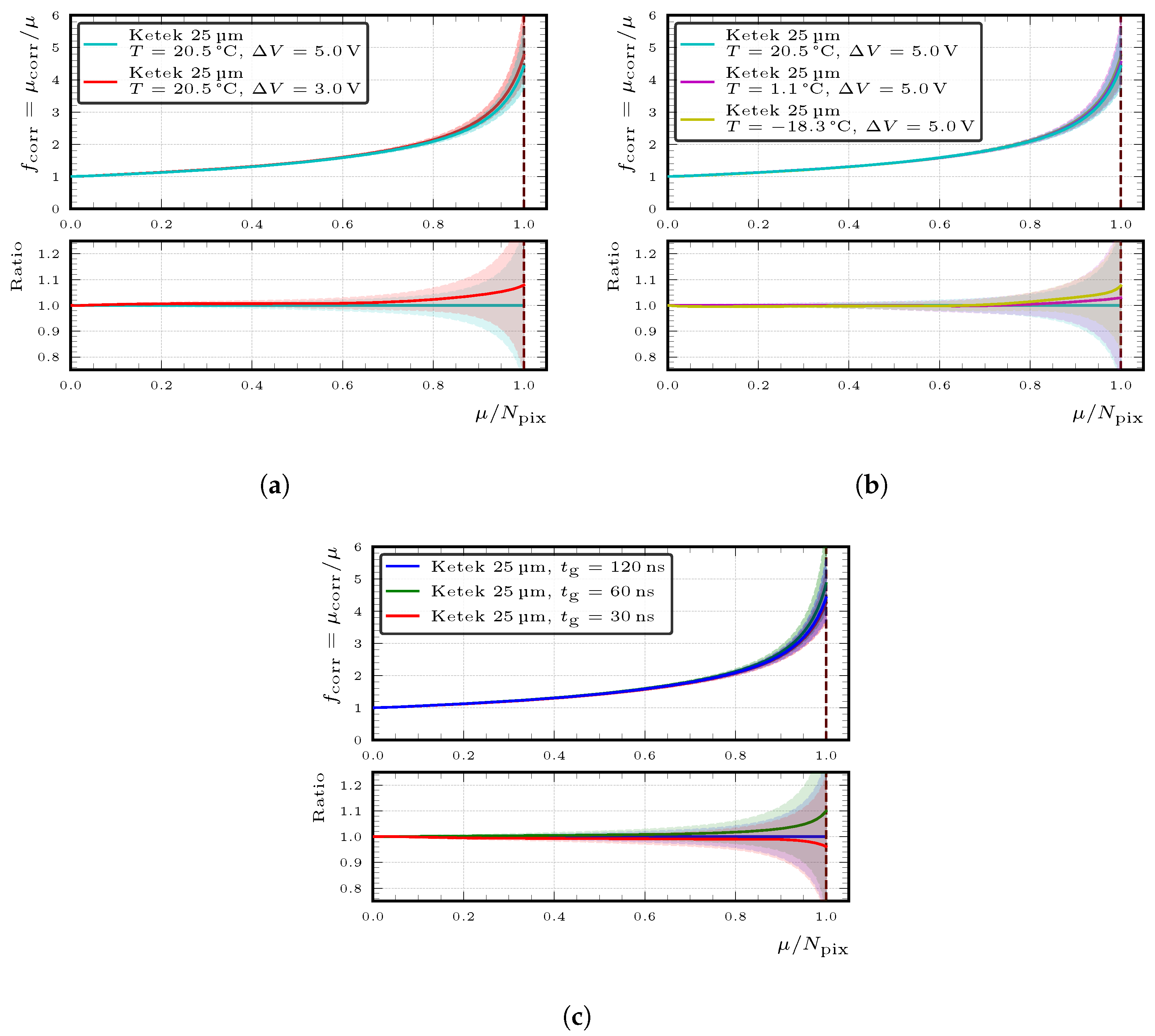
Once the effectiveness of the correction under varying conditions has been established, the variation of the correction function itself across the parameter space is examined. For the reference function to remain applicable, it must exhibit minimal variation when re-evaluated at different conditions. Figure 7 shows the correction factor introduced in Section 2 for the $25 \mathrm{\mu }\mathrm{m}$ SiPM determined at the reference point and the other extremes of the parameter space. The shaded bands represent the effect of a $2\%$ gain variation. The x-axis is normalised to the pixel count to enable cross-comparison between devices. The lower part of the plots shows the ratio to the reference curve ($T=20.5 °\mathrm{C}$, $\Delta V=5 \mathrm{V}$, $t_{\mathrm{g}}=120 \mathrm{n}\mathrm{s}$).

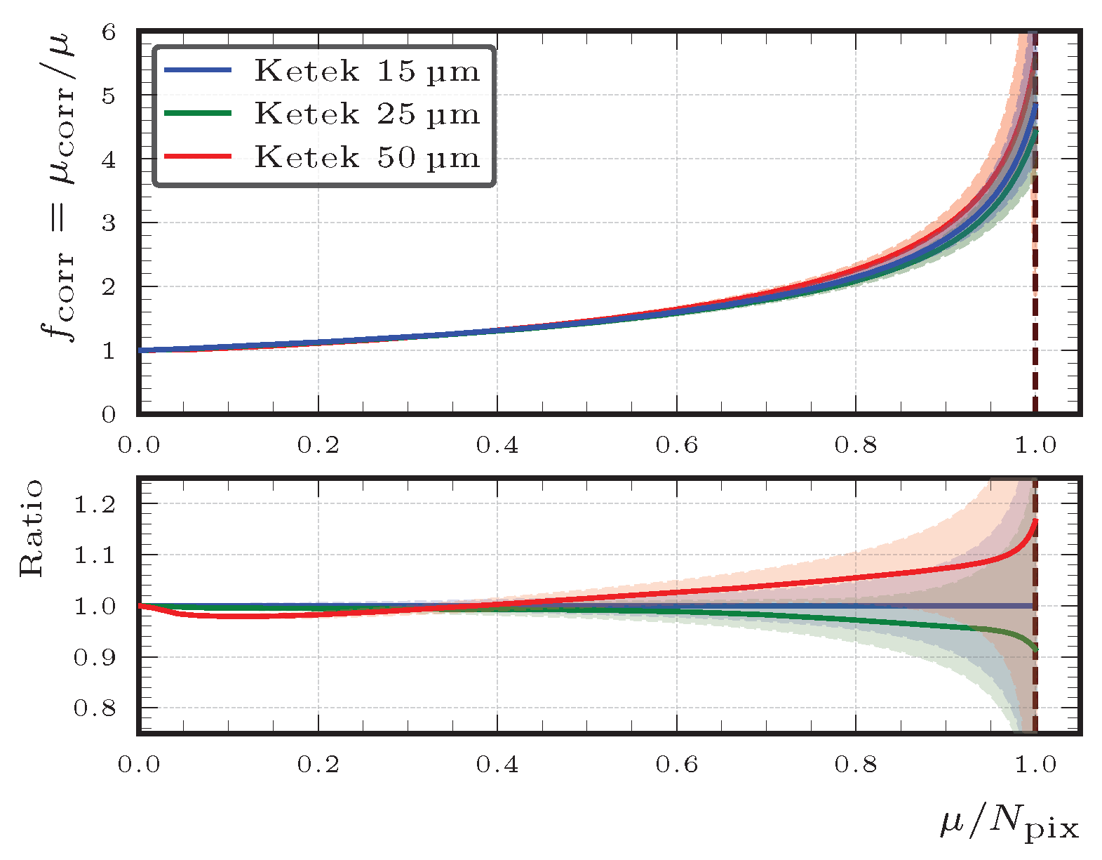
In Figure 7a, no significant dependence on the overvoltage at $T=20.5 °\mathrm{C}$ is observed, while Figure 7b shows no temperature dependence at a fixed overvoltage of $\Delta V=5 \mathrm{V}$. A factor of 2 is reached when the measured charge corresponds to $\approx 78\%$ of $N_{\mathrm{pix}}$ being hit. The last parameter we analysed to validate the correction factor is the integral gate length $t_{\mathrm{g}}$. Figure 7c shows the correction factor for the $25 \mathrm{\mu }\mathrm{m}$ SiPM taken at the reference condition, analysed with three different gate lengths $t_{\mathrm{g}}$ = 30, 60 and 120 ns. The gate length of $120 \mathrm{n}\mathrm{s}$ corresponds to an integration window that includes $96\%$ of the full gain, while the shorter gates of $60 \mathrm{n}\mathrm{s}$ and $30 \mathrm{n}\mathrm{s}$ include $78\%$ and $49\%$, respectively. Each time, the appropriate gain for that gate length was used. For the three chosen gate lengths, we do not observe a significant variation in the correction factor. Figure 8 shows the correction factor for each of the three SiPMs extracted at the reference conditions. For a correction factor smaller than 2, the difference between the different SiPMs is below $10\%$ and no ordering on pixel size is observed.

5. Conclusions

This work introduces a novel application of the single-step laser method for characterising and correcting the non-linear response of SiPMs at the event level. The correction curve, derived from measurements of three SiPMs with varying pixel sizes, demonstrates a high degree of universality, exhibiting minimal dependence on pixel size, overvoltage, temperature, and integration window. Importantly, the method effectively linearises the SiPM response across the entire operational range, including saturation levels exceeding $100\%$ pixel occupancy, with deviations below $3\%$. The correction improves upon the conventional correction based on a single-exponential model. Unlike most correction functions presented in the literature, this method can be applied on an event-by-event basis, for charges up to $q_0·G$ times the total number of pixels.

It is worth noting that the gain is not required for obtaining the correction function itself. For practical applications of the correction function, such as its use under different experimental conditions, knowledge of the gain at these conditions is nevertheless required. Deviations of around $2\%$ already have a significant impact at light intensities exceeding $N_{\mathrm{pix}}$.

The primary advantages of this approach are its independence from absolute light source calibration and its applicability under diverse operational conditions, simplifying large-scale detector calibration and enhancing their dynamic range. Consequently, this method could improve energy resolution and systematic accuracy of calorimetric detectors used in high-energy physics and medical imaging.

Future validations focus on validating the method across various SiPM types and vendors; results for one Hamamatsu Photonics device have already been published, confirming the validity of the method [19]. Future investigations will address the sensitivity of the correction to light source properties (time spread, wavelength, spatial distribution, and scintillator coupling) as well as the impact of radiation damage.

References

1. Laudrain, A. The SiPM-on-tile system of the CMS HGCAL. EPJ Web Conf. 2025, 320, 00041. [Google Scholar] [CrossRef]
2. CALICE Collaboration. Design, Construction and Commissioning of a Technological Prototype of a Highly Granular SiPM-on-tile Scintillator-Steel Hadronic Calorimeter. arXiv 2022, arXiv:2209.15327. [Google Scholar] [CrossRef]
3. Terragni, G.; Roux, L.; Delenne, J.; Bordelius, A.; Martinazzoli, L.; Pizzichemi, M.; Salomoni, M.; Roloff, P.; Gerasymov, I.; Viahin, O.; et al. Investigating the Application of Silicon Photomultipliers in Calorimetry: The Case Study of Spacal. In Proceedings of the 2025 IEEE Nuclear Science Symposium (NSS), Medical Imaging Conference (MIC) and Room Temperature Semiconductor Detector Conference (RTSD); IEEE: Piscataway, NJ, USA, 2025; pp. 1–2. [Google Scholar] [CrossRef]
4. Rubini, N.; Achari, B.R.; Agrawal, N.; Alexeev, M.; Alice, C.; Antonioli, P.; Baldanza, C.; Barion, L.; Calivà, A.; Capua, M.; et al. The SiPM readout plane for the ePIC-dRICH detector at the EIC: Overview and beam test results. Nucl. Instrum. Methods Phys. Res. Sect. A Accel. Spectrometers Detect. Assoc. Equip. 2026, 1082, 170890. [Google Scholar] [CrossRef]
5. Bisogni, M.G.; Del Guerra, A.; Belcari, N. Medical applications of silicon photomultipliers. Nucl. Instrum. Methods Phys. Res. Sect. A Accel. Spectrometers Detect. Assoc. Equip. 2019, 926, 118–128. [Google Scholar] [CrossRef]
6. Gundacker, S.; Heering, A. The silicon photomultiplier: Fundamentals and applications of a modern solid-state photon detector. Phys. Med. Biol. 2020, 65, 17TR01. [Google Scholar] [CrossRef] [PubMed]
7. Wang, L.; Wang, Y.; Wang, M. Energy calibration using scintillator background radiation for high-resolution PET detectors. Nucl. Instrum. Methods Phys. Res. Sect. A Accel. Spectrometers Detect. Assoc. Equip. 2020, 974, 164202. [Google Scholar] [CrossRef]
8. Auffray, E.; Hadj, F.B.M.B.; Cortinovis, D.; Doroud, K.; Garutti, E.; Lecoq, P.; Liu, Z.; Martinez, R.; Paganoni, M.; Pizzichemi, M.; et al. Characterization studies of silicon photomultipliers and crystals matrices for a novel time of flight PET detector. J. Instrum. 2015, 10, P06009. [Google Scholar] [CrossRef]
9. Gruber, L.; Brunner, S.; Marton, J.; Suzuki, K. Over saturation behavior of SiPMs at high photon exposure. Nucl. Instrum. Methods Phys. Res. A 2014, 737, 11–18. [Google Scholar] [CrossRef]
10. Kotera, K.; Choi, W.; Takeshita, T. Describing the response of saturated SiPMs. arXiv 2015, arXiv:1510.01102v4. [Google Scholar]
11. Bretz, T.; Hebbeker, T.; Lauscher, M.; Middendorf, L.; Niggemann, T.; Schumacher, J.; Stephan, M.; Bueno, A.; Navas, S.; Ruiz, A. Dynamic range measurement and calibration of SiPMs. J. Instrum. 2016, 11, P03009. [Google Scholar] [CrossRef]
12. Weitzel, Q.; Bernhard, P.; Brogna, A.; Degele, R.; Krause, S.; Schäfer, U.; Tapprogge, S. Measurement of the response of Silicon Photomultipliers from single photon detection to saturation. Nucl. Instrum. Methods Phys. Res. A 2019, 936, 558–560. [Google Scholar] [CrossRef]
13. Tsuji, N.; Ootani, W.; Liu, L.; Yoshioka, K.; Morita, Y.; Gonokami, M. Study on saturation of SiPM for scintillator calorimeter using UV laser. J. Instrum. 2020, 15, C05052. [Google Scholar] [CrossRef]
14. Han, D.; Liu, J.; Liang, K.; Dai, L.; Yang, R.; Cheng, W.; Peng, Y. Dynamic Range Characterization of SiPM with a Double Light Superposition (DLS) Method. Available online: https://indico.gsi.de/event/6990/contributions/31533/contribution.pdf (accessed on 3 February 2026).
15. Klanner, R. Characterisation of SiPMs. Nucl. Instrum. Methods Phys. Res. A 2019, 926, 36–56. [Google Scholar] [CrossRef]
16. Klanner, R. Simulation of the response of SiPMs Part II: With saturation effects. Nucl. Instrum. Methods Phys. Res. Sect. A Accel. Spectrometers Detect. Assoc. Equip. 2024, 1059, 169018. [Google Scholar] [CrossRef]
17. Renker, D.; Lorenz, E. Advances in solid state photon detectors. J. Instrum. 2009, 4, P04004. [Google Scholar] [CrossRef]
18. Antonello, M.; Brinkmann, L.; Freund, T.; Garutti, E.; Neumann, K.; Schwandt, J. Extending SiPM dynamic range with non-linear response correction: The single-step method. J. Instrum. 2025, 20, C08030. [Google Scholar] [CrossRef]
19. Brinkmann, L.; Garutti, E.; Martens, S.; Schwandt, J. Correcting the Non-Linear Response of Silicon Photomultipliers. Sensors 2024, 24, 1671. [Google Scholar] [CrossRef] [PubMed]
20. KETEK GmbH. Available online: https://www.ketek.net/ (accessed on 22 January 2024).
21. Brinkmann, L. Non-Linear Response of Silicon Photomultipliers. Master’s Thesis, Universität Hamburg, Hamburg, Germany, 2023. [Google Scholar]
22. Driesen+Kern GmbH. Available online: https://www.driesen-kern.de (accessed on 7 April 2025).
23. Antonello, M.; Brinkmann, L.; Garutti, E.; Klanner, R.; Schwandt, J. Is the gain–voltage dependence of SiPMs linear? Nucl. Instrum. Methods Phys. Res. Sect. A Accel. Spectrometers Detect. Assoc. Equip. 2025, 1076, 170444. [Google Scholar] [CrossRef]
24. Preamplifiers SiPM-High Performance | Advatech UK. Available online: https://www.advatech-uk.co.uk/preamps_sipm.html (accessed on 2 February 2025).
25. Gatti, E.; Piva, F. A new single channel elementary amplitude discriminator. Il Nuovo C. (1943–1954) 1953, 10, 984–985. [Google Scholar] [CrossRef]
26. Wright, A.G. The Photomultiplier Handbook; Oxford University Press: Oxford, UK, 2017. [Google Scholar]
27. Rolph, J.; Garutti, E.; Klanner, R.; Quadfasel, T.; Schwandt, J. PeakOTron: A Python module for fitting charge spectra of Silicon Photomultipliers. Nucl. Instrum. Methods Phys. Res. A 2023, 1056, 168544. [Google Scholar] [CrossRef]
28. Brinkmann, L.; Antonello, M. Dataset for Paper: Systematic Characterisation and Non-Linear Response Correction of SiPMs Using the Single-Step Method for High-Precision Calorimetry; University of Hamburg: Hamburg, Germany, 2026. [Google Scholar] [CrossRef]
Figure 1. Non-linear response measurement setup schematics.
Instruments 10 00024 g001
Figure 2. (a) The measured S ( μ ) as a function of the average μ . The blue dashed line is the fitted spline. The expectation from the simple exponential model Equation (1) is shown as the black line. The bottom part shows the residuals defined as the difference between the data and the spline or model, respectively. (b) The reciprocal of the measured S ( μ ) data and the spline from (a) as a function of μ . The horizontal dashed line represents a constant 1. Both for the 25   μ m SiPM at reference conditions defined in Table 2.
Instruments 10 00024 g002
Figure 3. Results of the gain scans for the 25   μ m sample, KETEK PM1125. (a) Gain versus bias voltage, (b) turn-off voltage versus temperature, and (c) gain versus gate length. The parameters of the fit functions to G V bias , d V off d T , and G t g are reported in Table 3 for all SiPMs investigated. The black circle marker in (a,c) indicates the reference conditions from which the parameter plotted on the x-axis is varied. In (b), the black circle represents the turn-off voltage determined in (a).
Instruments 10 00024 g003
Figure 4. Response functions of the three investigated SiPMs at the reference operating condition: T ref = 20   ° C , overvoltage Δ V ref = 5   V , and integration gate length t g , ref . (ac) correspond to 15, 25 and 50 μm pitch. The red curve ( μ 1 L ) is the uncorrected response, and the blue one ( μ 1 L , corr ) shows the linearised response after correction. The inset plots at the bottom right show the region of the response curve above the number of pixels in the devices, indicating that a small over-saturation is reached. (d) Comparison of the results from all three SiPMs shows that for high N seed values, responses slightly exceed the corresponding number of pixels.
Instruments 10 00024 g004
Figure 5. Deviations of the response function from the ideal linear response of the three investigated SiPMs at the reference operating condition: T ref = 20   ° C , overvoltage Δ V ref = 5   V , and integration gate length t g , ref . (ac) correspond to 15, 25 and 50 μm pitch. The red and blue data points show the deviation from a linear response before and after correction, respectively. The light blue band indicates the uncertainty from the correction function and the calculation of the deviation from linearity. The error bars indicate the uncertainty from the gain determination.
Instruments 10 00024 g005
Figure 6. Linearity score and dynamic range extension factor when the correction taken at reference operating condition: T ref = 20   ° C and overvoltage Δ V ref = 5   V , is applied to data taken within the parameter space. (ac) correspond to 15, 25 and 50 μm pitch. The upper number in each cell shows the linearity score, the bottom number the dynamic range extension factor. The colour indicates the linearity score.
Instruments 10 00024 g006
Figure 7. Comparison of the correction factor, defined in Equation (9), for the 25   μ m pitch SiPM. The colour band shows the impact of a 2 % change of the gain. (a) Correction factor at reference temperature T set = 20   ° C for overvoltages ΔV = 3, 5 V. (b) Correction factor at fixed overvoltage Δ V = 5   V for set temperatures T set = −20, 0, 20 °C. (c) Correction factor at the reference condition analysed with different gate lengths t g = 30, 60 and 120 ns. The lower panel shows the ratio of each curve to the reference curve at T = 20.5   ° C , Δ V = 5   V , and t g = 120   n s .
Instruments 10 00024 g007
Figure 8. Comparison of the correction determined at the reference condition for all three SiPMs with different pixel pitches 15, 25 and 50 μm. The lower plot shows the ratio with respect to the 15   μ m SiPM.
Instruments 10 00024 g008