Application of Machine Learning for Predicting the Abundance of Russian Sturgeon in the Sea of Azov Based on Historical Annual Ecosystem Dataset

Abstract

A new approach was applied for forecasting purposes of Russian sturgeon abundance in the Sea of Azov. Different types of supervised machine learning models were tested based on long-term data of Russian sturgeon abundance and ecosystem parameters of the Sea of Azov during the period 1970–2024. The best determination and the smallest mean average error were achieved by a random forest model. Among the neural networks, the Bayesian regularized neural network model showed good fitting, but it lost in accuracy against the random forest. Boosting-type models did not show a significant advantage in comparison with classic additive models. The reliability of the obtained solution using the random forest model surpassed the previously obtained results of the production model and was at the level of a cohort solution. The use of the random forest model made it possible to describe the period of depletion of the Russian sturgeon population in 2000–2024, in contrast to analytical models. Based on the results of the model type selection, a few sub-models were fitted for each ecosystem sector (or predictor selection technique): Full, Toppred, Hydro, and Food models to make predictions possible in the theoretical case of missing data. The best fitting and most accurate diagnostics were achieved by the Full (R² = 0.84, Adj.R² = 0.79) and Toppred (R² = 0.75, Adj.R² = 0.73) models. The Hydro sub-model also seems suitable (R² = 0.68, Adj.R² = 0.65) to predict Russian sturgeon abundance. Short-term forecasts were performed after the introduction of lags between ecosystem predictor factors and predictable sturgeon numbers (lag = 4 years). The Full, Toppred, and Food models predict a significant increase in the number of Russian sturgeons during 2025–2026 (up to ~5 M specimens), whereas the Hydro model predicts a decrease (sturgeon numbers in the range of 0.2–1.4 M specimens).

1. Introduction

The Russian sturgeon (Acipenser gueldenstaedtii) in the Sea of Azov is a long-living fish species, with life expectancy in some historical periods reaching 60–100 years. The history of Russian sturgeon in the Sea of Azov can be described in terms of various periods that impacted the abundance of population and reproduction conditions [1,2]. Before the 1950s, the Russian sturgeon was the most numerous species in the Sea of Azov [3]. The main drivers of population changes in this species throughout history have been fishing and the construction of hydroelectric complexes on the Don River, which is the main spawning area for this species. The first decline occurred after the construction of the Tsimlyansk Hydroelectric Complex in 1952, which led to the near-complete loss of natural reproduction opportunities by the 1970s and 1980s. Overfishing and high levels of illegal, unreported, and unregulated (IUU) fishing during the mid-1990s led to a second decline in the population abundance of the Russian sturgeon. Since the 2000s, commercial fishing for this species has been completely banned due to extremely low population numbers [4,5,6,7]. However, there have been some indications of a slight recovery in the sturgeon population since 2020 [2,7].

The stock assessment of Russian sturgeon has been assessed in various ways through time. Traditionally, these estimates were performed using the swept area method (SA), and forecasting was done using the Baranov equation based on assumptions about mortality, recruitment process, and population structure [7,8,9]. Subsequently, approaches of surplus production [10] and cohort modeling [11] of Russian sturgeon population dynamics were proposed in the period when the population had a commercial status (1980–2000). Recently, some kind of modified SA, including trap-nets data, has been used to assess the stock, taking into account the by-catches of Russian sturgeon in coastal fishing gear [12]. Despite the diversity of methods for estimating the stock of Russian sturgeon, currently, in the absence of fishing and catch statistics after 2000, only the SA of direct accounting has been applicable to forecasting.

However, the SA method has some accuracy restrictions [13,14]. The main one relates to the ability to catch and count fish using fishing gear. Due to low abundance, non-uniform spatial distribution, and spatial distribution uncertainty, the application of SA since the 2000s has had significant accuracy issues. Additionally, the low abundance and uneven spatial distribution make it difficult to perform short-term forecasts. Additionally, the use of modified surplus and cohort models continued to present challenges during the modern non-fishing period between 2000 and 2025. For this reason, it is difficult to build any forecasts without tuning relevant population parameters during this modern period. The transition from natural to artificial reproduction in fish hatcheries further complicates this task.

In such conditions, it is necessary to develop a fisheries-independent method based on long-term observations from the historical period in order to estimate the abundance of Russian sturgeon. This method would be beneficial in situations where it is impossible to conduct surveys to calculate swept area estimates due to weather conditions, fishing gear, or other factors. It would allow for a more accurate assessment of sturgeon populations and provide reliable information for decision-making.

The objective of this research was to develop models based on long-term ecosystem observations in order to predict the number of Russian sturgeons. The main hypothesis was that regression models, fitted on retrospective ecosystem data, such as analytical or machine learning approaches, would be able to adequately describe population abundance dynamics. To test this hypothesis, the following tasks were performed:

-

Prepare a long-term dataset of available annual data on the demersal species in the Sea of Azov;

-

Test linear, non-linear, and machine learning regression models using the full dataset to predict Russian sturgeon abundance based on retrospective data;

-

Select the model with the best accuracy metrics and perform statistical diagnostics on it;

-

Reduce the number of available factors in the model by ecosystem sectors to make predictions available in cases where data are lacking;

-

Introduce shifts between ecosystem factors and predicted Russian sturgeon numbers based on retrospective data to create a short-term forecast.

2. Materials and Methods

2.1. Study Area

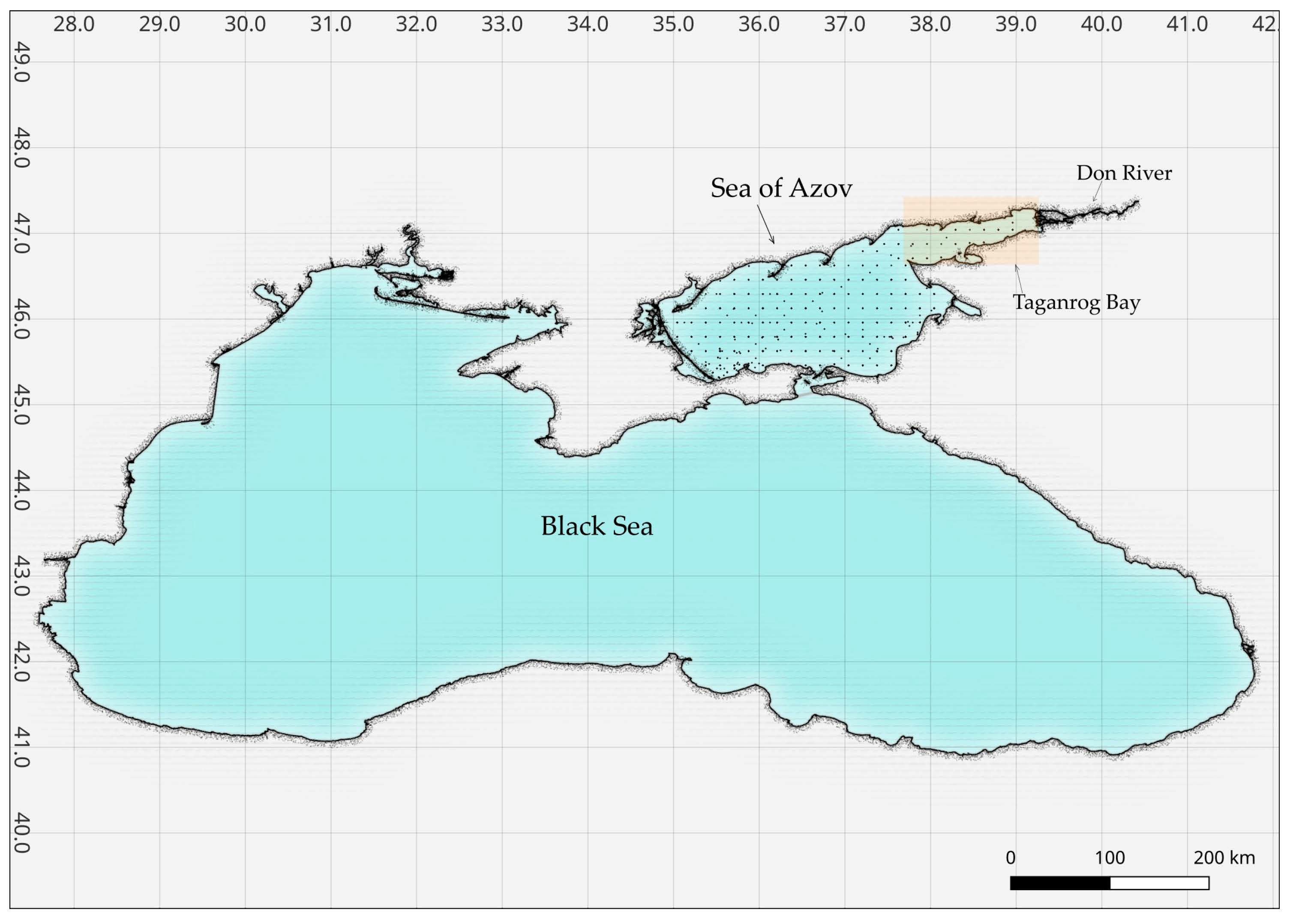
The study area was located between south-west part of Europe and the peninsula of Asia Minor. The reservoir of the Azov Sea is connected to the Black Sea by the narrow isthmus of the Kerch Strait (34.5 W ~ 39.5 W, 45.0 N ~ 47.5 N, Figure 1). The Sea of Azov is a native Russian sturgeon habitat.

2.2. Data

The Azov Sea ecosystem dataset used in this research was previously published [15] and described in a manuscript [16]. The published retrospective data were average annual estimates of biotic and abiotic indicators of the Sea of Azov for the period 1925–2024. The dataset contains annual evaluated factors related to the Russian sturgeon ecosystem: hydrology (total annual Don River flow volume, average summer sea surface temperature in summer from in situ observations, average annual water salinity in the Taganrog Bay and Sea of Azov), food chains (relative zooplankton biomass during the summer period, relative zoobenthos biomass and forage fraction biomass in autumn), demersal fishes biomass and catches (sander, gobies, rutilus biomass and catches), and hatchery production (Russian sturgeon hatchery annual release numbers for the Don and Kuban Rivers). As predictable variable, the numbers of Russian sturgeon were used to train our models.

In order to fit various machine learning models, taking into account the completeness and omissions in the dataset, the period 1970–2024 was chosen. The period selection was also determined by the biological meanings of the Russian sturgeon reproduction shift: after 1970, there was low or absent natural spawning detected and the main replenishment was due to artificial reproduction. Before 1970, natural spawning in limited areas existed, and for modelling these can involve misfitting on parameter weight evaluation [2].

The complete dataset for the period 1970–2024 contains only 55 variables for each ecosystem factor. From the machine learning side this dataset is tiny, and special tuning should be applied to avoid overfitting issues. However, the machine learning approach has previously been applied in similar tiny dataset conditions for marine ecosystems, starting from 10 variables [17,18,19].

2.3. Data Pre-Processing

Preprocessing of data was carried out when implementing the machine learning models and classic regression models. Data series were smoothed, centered, and transformed using the Yeo–Johnson method [20,21].

2.4. Model Selection

The model selection process and model fitting were performed in the R environment(version 4.5.2) using the caret package (version 7.0.1) [22,23].

One model for each different type of supervised learning was selected as the candidate model. The classic regression solution was trained. Next, several models were tested: a random forest (RF), a classical neural network (NNET), a Bayesian regularized neural network (BRNN), a generalized model boosting (GLMBoost), and a Bayesian implementation of generalized linear models (BayesGLM).

When training the models, the regression of all available ecosystem factors (predictors) was used to predict the number of Russian sturgeon (predictable). During the training process, a retrospective dataset was split into training and validation subsets. The training subset comprised 80% of the data, while the validation subset comprised 20%. The model’s validation was performed on an independent validation dataset that was not used for training.

The training was performed using the repeated cross-validation (repeatedcv) method with the technique of selecting validation subsamples (1/5 of dataset, numbers = 5, repeats = 5) using the folding knife method. When training the models, parameterization was performed, which made it impossible to overfit (overlearning problem) the models taking into account the small size of the dataset (ntrees < 50; neurons < 20) [24].

In order to compare machine learning and classic models, three regression models were implemented: a linear regression model (LM), a generalized linear regression model (GLM), and a generalized additive model (GAM) [25].

The selection of the best fitting model was based on a combination of three main metrics for diagnosing regression models: the coefficient of determination (R²) of a test subsample of data, the lowest mean average error (MAE) values, and the lowest root mean squared error (RMSE) values.

In the case of model comparison, the adjusted R² was calculated based on the number of predictors and the length of the dataset:

$$\mathrm{A}\mathrm{d}\mathrm{j}.{\mathrm{R}}^2=1-(1-{\mathrm{R}}^2){\displaystyle \frac{\mathrm{n}-1}{\mathrm{n}-\mathrm{p}-1}}$$

where:

R²—the determination coefficient of model fit,

n—the number of observations,

p—the number of predictors.

The interpretation of R² values in human-friendly rankings is a complicated statistical issue that requires providing clear advice on model performance [26]. Currently, there is no unified ranking scale available for stock assessment research. In this case we used the following: high rank at R² > 0.75, moderate rank at R² = [0.5; 0.75], and low rank at R² < 0.5. However, all R² model metrics in this paper emphasize a significant parameter fit from a statistical perspective (t-test at significance level a = 0.05). The decision about model performance was always based on RMSE and MAE.

2.5. Time-Series Time-Block Model Validation

In the case of time-series assessment, a common approach is the rolling forecasting origin technique. Instead of cross-validation with repeatedcv, this approach is based on non-independent assumptions about data series over the time vector. Using this approach, training and validation subsamples are continuously separated over the time vector, with each next value x_t depending on the previous value x_t−1. Due to the nature of this approach, there is a significant connection between subsequent values in the time vector that may be lost through random re-sampling or lead to false validation through random subsets [27].

To verify this assumption and avoid misfitting or mis-validation by repeated cross-validation, the time-series dependent approach was tested for the random forest model. Time-series slices were prepared using the caret package with two main parameters: the initial window size (the number of consecutive values in the training sample) and the forecast horizon (the test sample size). The forecast horizon was set at 3 years (short-term forecasting requirements), and the initial window size was calculated iteratively in a range from 10 to 50 values.

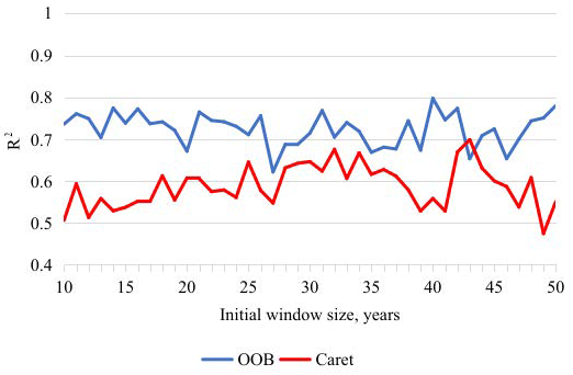
In trainControl, the timeslice method was used. Two metrics were calculated: the R² from the OOB (out-of-box) single random forest trained model and an independent caret estimate of R². The OOB R² represents an error calculation internally during the forecast construction process, while the caret R² evaluates a “past predict feature” strategy based on average errors across the forecast horizon.

2.6. Sub-Model Tuning

The following sub-models were developed to fit different sets of habitat parameters, depending on the part of the ecosystem they describe (

Table 1. The stack of predictors by different ecosystem parts for modeling Russian sturgeon abundance numbers.

Model	Full	Hydro	Food	Toppred
Predictors set	Don River flow volume, Azov Sea & Taganrog Bay salinity, Avg sea summer water surface temperature, Relative biomass of zoobenthos & zooplankton, sander, gobies, rutilus biomass, Russian sturgeon hatchery annual release numbers	Don River flow volume, Azov Sea & Taganrog Bay salinity, Avg sea summer water surface temperature	Relative biomass of zoobenthos & zooplankton	Gobies stock biomass, Avg sea summer water surface temperature, Russian sturgeon hatchery annual release numbers

). The top predictors (Toppred) model, which was developed after training, highlights the most significant factors from the full model.

2.7. Models Diagnostics

Traditional summary diagnostics were calculated for each model: classic and adjusted determination (R²), mean root squared error (RMSE) and mean average error (MAE). The final decision about the best fitting was taken based on maximizing R² and minimizing RMSE and MAE.

For each sub-model in the dataset, there were differences in the swept area estimates based on the predictor stack. In this case, “diffs” was a deviation from the estimates of Russian sturgeon numbers by the SA method (N_sa) in each year (t) of the dataset and the numbers fitted by the model (N_m):

diff_(t) = N_m(t) − N_sa(t)

(1)

Indeed, this “diffs” is actually a measure of difference between the swept area sturgeon numbers estimates and this value fitted by the models. However, this simple metric can provide valuable information about model discrepancies between the number of Russian sturgeons and the traditional SA. Some meanings can be investigated based on the patterns of this diffs distribution by the time vector. Finally, the absolute sum of diffs regarding to the length of time series can provide simple weight metrics of mean estimation error (in addition to MAE metrics):

error_N = sum(abs(diff_(t)))/count(diff_(t))

(2)

2.8. Lags and Forecast

A feature of models based on learning from historical data is the requirement for the values of all predictors to produce a forecast. However, it was impossible to predict the average annual temperature or Don River flow volume and other ecosystem parameters with high accuracy. Nevertheless, the long-term relationship between the numbers of Russian sturgeon and environmental indicators was obvious.

Considering the long-term impact of habitat parameters on sturgeon populations and the availability of predictive models, the lags between predictors (ecosystem factors) and predicted values (sturgeon numbers) was introduced. As shown in our research on gobies in the Sea of Azov using a random forest model, a lag of up to 4 years did not significantly reduce R² or other metrics [28].

3. Results

3.1. Model Testing and Selection

A summary of the main metrics of model type selection is presented in

Table 2. Model type selection of Russian sturgeon numbers based on the parameters of the ecosystem of the Sea of Azov for the period 1970–2024.

Model	R2	Adj.R2	MAE	RMSE
LM	0.47	0.33	3147	3883
GLM	0.46	0.32	3194	4126
GAM	0.53	0.41	3123	4278
RF	0.84	0.79	1852	2258
NNET	0.39	0.24	4953	6689
BRNN	0.75	0.68	2130	2772
GLMBoost	0.59	0.48	2711	3145
BayesGLM	0.59	0.48	2733	3314

. The most reliable classic regression models (LM, GLM, GAM) were additive GAM models with a low determination of Adj.R² = 0.41. Among the models of machine learning, the best results were found in the RF model, Adj.R² = 0.79. At the same time, the BRNN model demonstrated a moderate determination, Adj.R² = 0.68.

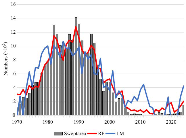
Visualization of the Russian sturgeon number estimates based on the swept area method and RF and LM models are shown in Figure 2. When comparing two models, it is clear that the RF model provided more accurate results for describing population dynamics than the LM model (Table 2). In addition to its high accuracy, the RF model also showed smaller discrepancies compared to the multiple linear regression model.

When comparing estimates of the number of Russian sturgeons made by the LM and RF models, it is worth noting the low reliability of the LM in the 1990–2005 period. During this time, its estimates had an incorrect trend and, biologically speaking, were meaningless in some years (2014–2018), falling below 0. At the same time, the RF model showed no significant anomalies or discrepancies with previous estimates even during these periods.

As expected, the machine learning models showed higher decision accuracy than the classic regression models. The high determination of the RF model has already been shown in solving a similar problem of predicting the biomass of the stock of gobies in the Sea of Azov [28].

In this regard, the RF model was chosen as the basis for the forecast and sub-model tuning to investigate ecosystem impact separately by sector.

3.2. RF Model Diagnostics

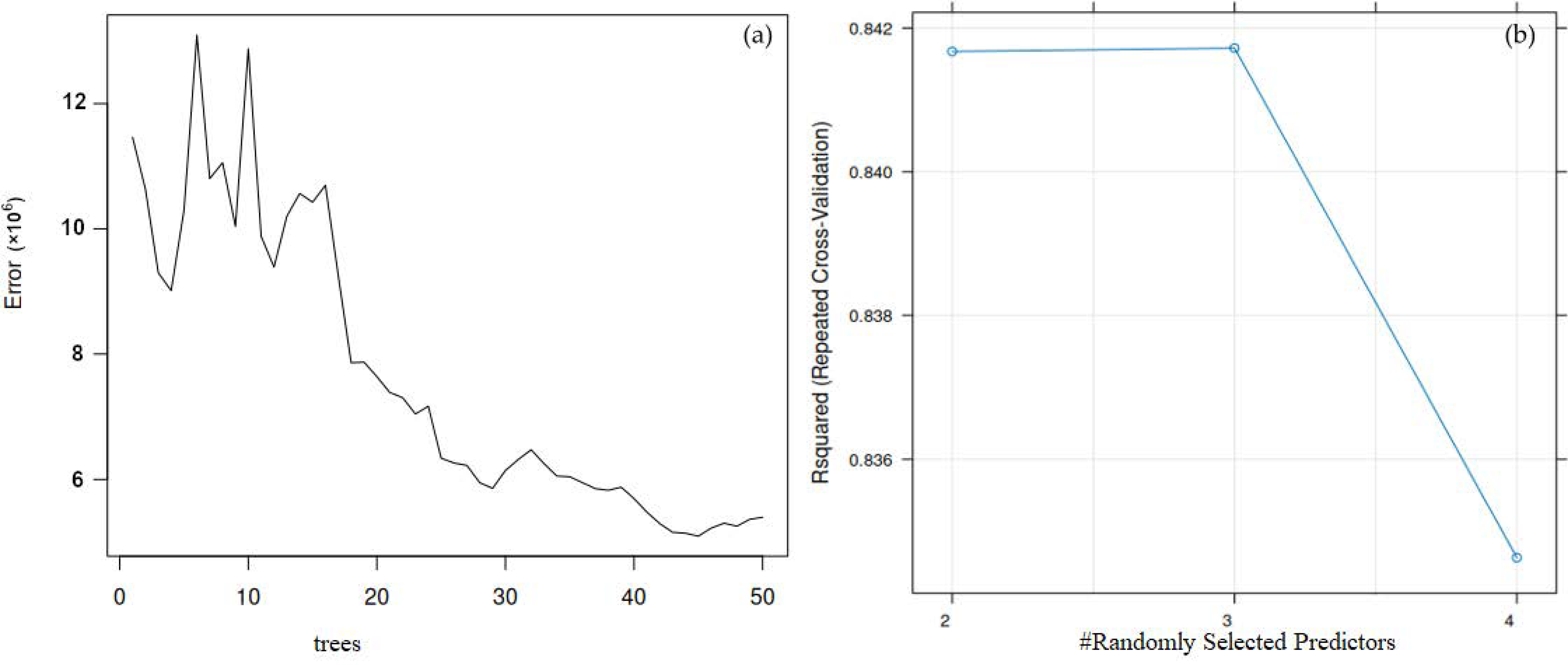
The basic RF model diagnostic, process error analysis by tree numbers, and the selection of the optimal number of predictors are shown in Figure 3. Process error diagnostics show high error values only when the number of trees was lower than 30. After 30 trees, there was no significant difference in process error. R² changes in cross-validation, depending on the randomly selected number of predictors, show a slight decrease in determination after 3 randomly selected predictors in the forest building process from trees.

The main metrics of the full model show suitable accuracy and high determination to predict the numbers of Russian sturgeon across the historical period (Adj.R² = 0.79, MAE = 1852, RMSE = 2258). The “top predictors” among the full ecosystem factors, with regression weights scaled to 0 … 100, are presented in

Table 3. Top predictors (weights scaled to 0 … 100, variable importance of RF) of full RF model by Sea of Azov ecosystem predictors to predict Russian sturgeon numbers.

Predictor	Importance
Gobies annual stock fishery biomass	100.0
Azov Sea summer average surface water temperature	57.5
Russian sturgeon hatchery annual release numbers	48.1
Sander annual stock total biomass	30.8
Annual average water salinity of the Azov Sea	26.8
Annual average Taganrog Bay water salinity	13.6
Relative biomass of zoobenthos forage fractions	12.4
Relative biomass of zooplankton	10.4

.

The obtained results indicate no evidence to reject the RF model for the full set of predictors. In this case, future investigation and splitting ecosystem predictors by sector was performed.

3.3. Time-Block Model Validation

In assumption of time-depended data validation, time-block tuning was applied instead of repeatedcv in Section 3.1 and Section 3.2 to the random forest model with the full dataset. The R² estimates by OOB and caret’s “past predict feature” presented in Figure 4.

As can be seen in Figure 4, time-block tuning results in a decrease in the model’s determination to a moderate level. However, the maximum observed determination, depending on the choice of the initial window size, in some cases reaches the levels indicated in Table 2. Maximum OOB R² = 0.80, Adj.R² = 0.72 (at initial window = 40); for caret’s “past predict feature” maximum R² was 0.70, Adj.R² = 0.60 (initial window = 43). Such determination indicates a decrease in performance relative to the repeatedcv method (Table 2), while parameterization of this approach significantly complicates the final solution and the number of varying parameters in it.

However, no significant evidence of the unreliability of the considered approach was found. For this reason, we decided to use the repeatedcv method to build models with the introduction of lags and sub-model tuning.

3.4. Sub-Model Tuning

As described in Section 2.6, to evaluate the opportunity to predict Russian sturgeon numbers by different sectors of the ecosystem, hydrology (Hydro), food-chain (Food) and top predictors (Toppred) sub-models were fitted by RF. The main metrics of fitting these models are presented in

Table 4. The full model and sub-models by ecosystem sector diagnostics comparison.

Model (or Sub-Model)	R2	Adj.R2	RMSE	MAE
Full	0.84	0.79	2258	1852
Hydro	0.68	0.65	2760	2215
Food	0.45	0.41	3628	3029
Toppred	0.75	0.73	2355	1776

.

The full model shows high determination and the lowest RMSE and MAE metrics, which include all ecosystem factors in order to explain the dynamics of Russian sturgeon numbers. The model based on the top predictors from the full model achieved high determination, according to the full model, with an R² = 0.75. Nevertheless, with close Adj.R² values, the MAE was lower than that of the full model, which was likely due to the reduction in noise caused by reducing the number of significant predictors.

The hydrology model showed sufficient accuracy and moderate determination (Adj.R² = 0.65), but its MAE was slightly higher than that of the full model and the Toppred sub-model. The model based solely on food chain components of the ecosystem was outside of this range, with a low determination, Adj.R² = 0.41.

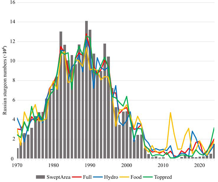
The prediction of historical numbers of Russian sturgeon by each of the RF sub-models is summarized in Figure 5. As can be seen, all models have a satisfactory explanation of Russian sturgeon population dynamics over the period 1970–2024. A detailed review of the estimates from the fitted models reveals some patterns:

•

For the period 1970–1975, all models gave higher estimates of Russian sturgeon numbers compared to the SA evaluation;

•

For the period 1976–1996, all of the models gave lower values of Russian sturgeon numbers estimate than the SA did;

•

For the period since 2005, all of fitted models produced overestimates compared to the SA;

•

For the period 2005–2024, the Food and Hydro sub-models showed the worst precision compared to the SA values.

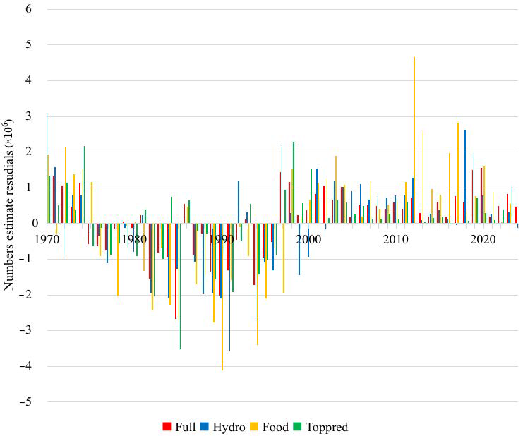
To provide detailed investigation of detected mis-fitting patterns, diffs diagnostics (base line—SA estimates) was performed using Equations (1) and (2). A diffs visualization is presented in Figure 6.

The patterns that were previously noted were fully supported by the diffs diagnostics. All RF sub-models showed three periods with different pattern of diffs: positive during 1970–1975, negative diffs during 1976–1996, and positive diffs during 1997–2024.

3.5. Lags and Forecast

After the introduction of lags between predictors (ecosystem factors) and predictable factors (Russian sturgeon numbers), the sub-models were fitted again, with the general diagnostics shown in

Table 5. The full model and sub-models by ecosystem sector diagnostics comparison with a lag of 4 years.

Model (or Sub-Model)	R2	Adj.R2	RMSE	MAE
Full	0.83	0.78	2401	1999
Hydro	0.68	0.65	2810	2326
Food	0.48	0.43	3633	2955
Toppred	0.71	0.69	2582	1951

. As expected, there was no significant reduction in performance against the models without lags: determination was still at a high level for the full model, at a moderate level for Hydro and Toppred, and at a low level for Food (compare Table 4).

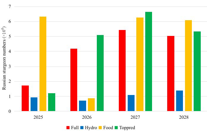
A short-term forecast of Russian sturgeon numbers based on the introduction of lags was performed, as shown in Figure 7. The obtained results differ significantly in the numbers of sturgeon forecast.

The Food sub-model provided the most optimistic forecast among the models. According to the Food model, the number of Russian sturgeons might reach 6.2–6.3 M specimens. That seems to be a realistic estimate based on the food source of sturgeon. The available benthic feed base is currently significantly underutilized because of the low stock biomass of benthic fishes. The unconsumed part of the forage fraction of zoobenthos was around 85 g/m² average during the last 20 years (for total zoobenthos biomass—more than 600 g/m²).

The Hydro sub-model offered a pessimistic scenario for the future trend of Russian sturgeon population abundance. The model, based on hydrological conditions, predicted sturgeon numbers of between 0.72–1.4 M specimens. This prediction contradicts the Food sub-model forecast.

Finally, the full model and the Toppred sub-model showed the closest predictions and highest determination of all. The full model predicted a strong increasing trend for the numbers of Russian sturgeon, from 1.7 M in 2025 to 5.0 M specimens in 2028. The same trend appears in the Toppred sub-model, with the numbers of Russian sturgeon increasing from 1.2 M in 2025 to 5.3 M in 2028.

4. Discussion

The objective of this research was to develop models based on long-term ecosystem observations in order to predict the number of Russian sturgeons. The main hypothesis was that regression models, fitted on retrospective ecosystem data, such as analytical or machine learning approaches, can adequately describe population abundance dynamics. Based on this we have obtained certain results, the discussion of which is given in this section.

4.1. Model Selection and Diagnostics

The RF model was shown to outperform classic regression models such as linear regression, generalized linear models, and general additive models in solving regression tasks, and other machine learning models such as neural networks, Bayesian GLMs and boosting techniques.

It should be noted that when trying to apply the model approach earlier (production and cohort models), modeling was applicable only for the well-studied period of the Russian sturgeon population, 1980–2000. The choice of this period was due to the non-commercial status of the population since 2000 (lack of catch statistics), high IUU fishing, and fluctuations in the survival rate of juveniles released from hatcheries. Under such conditions, production and cohort models did not allow us to describe the dynamics of the population during the period 2001–2024 and made it difficult to predict the population number due to the large gap in the data [10,11].

The RF model allowed us to obtain representative estimates of the sturgeon population for the period 2001–2024 (Figure 2), which was undoubtedly a significant advantage over the previously presented analytical solutions.

Previously, when implementing analytical models for the limited retrospective period of 1980–2000, the following determination parameters were obtained: for the modified surplus production model—R² = 0.73, MAE = 2776, and for the cohort—R² = 0.83, MAE = 1908 [11]. The obtained diagnostics for the RF model in this work surpass the production solution and are close to the reliability parameters of the cohort solution. Moreover, the RF model describes a much longer historical period of 1970–2024 than previously performed analytical solutions (modified surplus production model—1980–2000, cohort model—1985–2004).

The RF diagnostics (Figure 3) indicate suitable ecosystem parameters selection, which minimizes process errors and finds the optimums for tree builds. Despite the small sample size and limited model tuning to avoid overfitting issues, the determination of the full model was high (R² = 0.84), indicating sufficient model accuracy.

4.2. Model Variable Importance

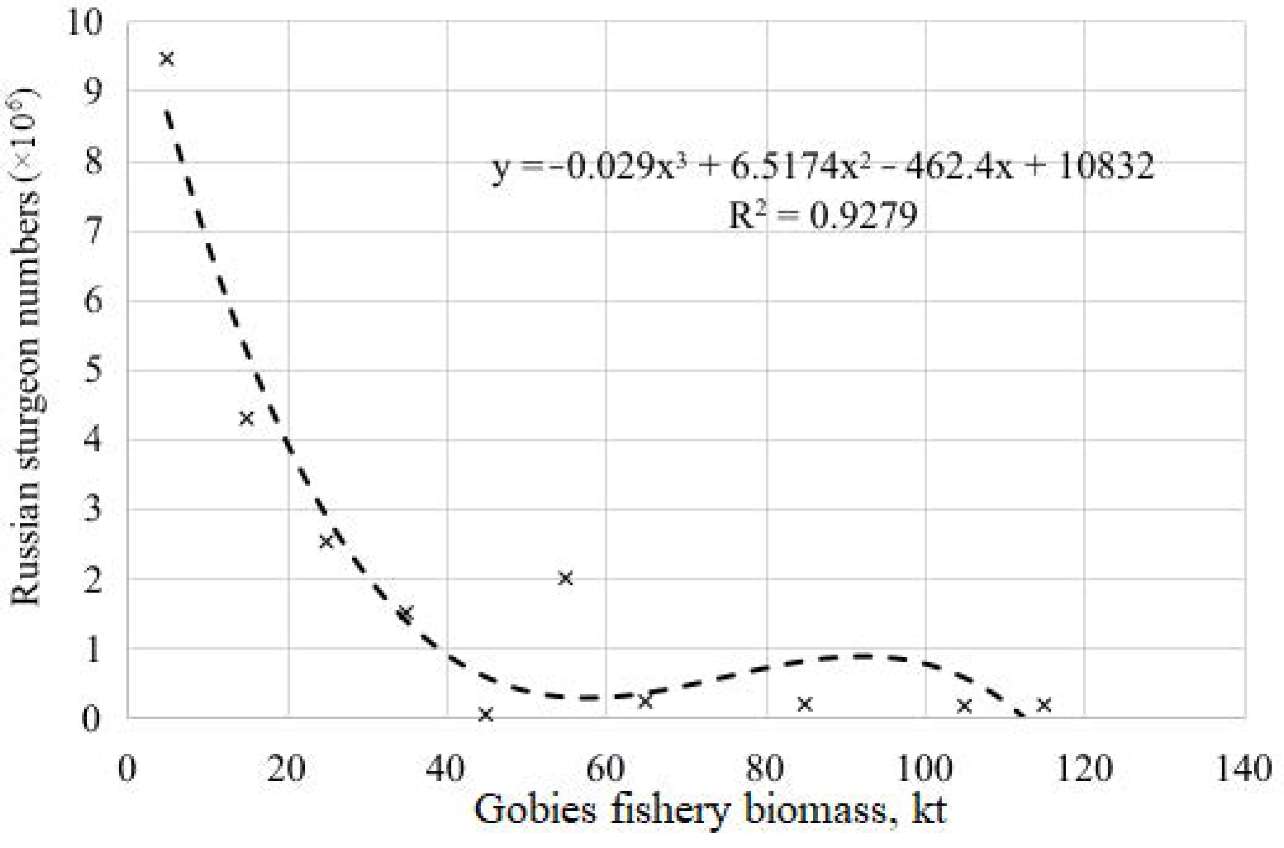
The variable importance of the full model (top predictor factors, Table 3) requires detailed discussion. The most important predictor was the gobies fishery stock biomass. Research about Russian sturgeon diet has been carried out during the past century [29,30,31]. One study noted that gobies make up more than 20% of the diet of Russian sturgeon. In shelf areas close to shoreline and in the Taganrog Bay, this figure can rise to 57%. Studies indicate that small gobies are important for feeding sturgeons in the early life cycle (2–4 years). The ad-hoc regression analysis (Figure 8) revealed a significant relationship between these ecosystem components and high determination.

Figure 8. Russian sturgeon numbers and gobies fishery stock biomass (grouped by 10 kt), polynomial regression (3rd order).

Figure 8. Russian sturgeon numbers and gobies fishery stock biomass (grouped by 10 kt), polynomial regression (3rd order).

In this way, the biomass dynamics of gobies seems to be a good predictor of Russian sturgeon abundance, as it reflects some aspects of their predator–prey relationship. However, it should be noted that a spurious correlation may occur in the case of the secondary status of gobies in the sturgeon’s diet.

The general diet of Russian sturgeons is very varied. During different stages of their life cycle, they can feed on mysids, worms, crabs, shrimps, small mussels, and zooplankton. This means that when the biomass of gobies is low, it may not be easy to predict or explain the number of sturgeons. Perhaps there is another factor that affects the dynamics of both sturgeon and goby populations during periods with low goby biomass.

The other top predictors of variable importance in our full model are easier to explain. The average sea summer surface water temperature indicates not only warmer years, but also the length of the growing season. Higher values usually indicate a longer growing season. The hatchery releases of Russian sturgeon have a direct impact on the population of sturgeons in the Sea of Azov due to the lack of natural spawning.

4.3. Sub-Model Discussion

The performance of sub-models and models with shift diagnostics (Table 4 and Table 5) look biologically and logically correct. Reduction in predictor numbers decreased determination and increased MAE and RMSE. Likewise, the accuracy and determination of the Food sub-model was low. This is not surprising, as throughout the history of research, no evidence of a lack of food for Russian sturgeon in the Azov Sea has been reported [2]. In other words, the food supply has never been a limiting factor for Russian sturgeon in the Sea of Azov.

In contrast to the Food model, the Hydro model, based on hydrological ecosystem factors, seems to be sufficient to explain sturgeon numbers with moderate determination. This is surprising, because Russian sturgeons can grow in waters with salinity up to 18 ‰ and a wide range of temperature fluctuations. Only natural spawning occurs in fresh waters, but during the 1970–2024 period, sturgeon populations saw no natural spawning. Hydrological conditions seem to be secondary to a stack of other ecosystem factors. However, water salinity and temperature act as intermediate factors in the duration of the growing season and the composition of zooplankton and zoobenthic species.

Ultimately, the full model and the Toppred sub-model exhibited good fit with high accuracy and high and moderate determination respectively, even when there were lags introduced. However, the accuracy of the Toppred sub-model decreased when the number of available ecosystem factors was reduced. However, this decrease is not essential, and the model can still be used in situations where data are limited.

Another point worth noting is the significant discrepancy between the estimates from all RF sub-models and those from the SA method during the period 2008–2019. During this period, the abundance of Russian sturgeon was very low. Under such conditions (extreme low and extreme high values), all models performed poorly, and the swept area method significantly underestimated the population abundance.

An interesting pattern was discovered during analysis of the sub-model estimates of sturgeon numbers compared to SA estimates (and their diffs, Figure 5 and Figure 6). The diffs show three periods with different patterns of diffs distribution. For 1970–1975, the models predicted higher numbers than SA, while for 1976–1996 the opposite was true, and for 1997–2024 the models again predicted higher numbers than SA. The explanation may be due to inaccuracies in the SA method or the impact of IUU fisheries. For the first period (1970–1975), there may have been higher sturgeon numbers at the beginning of the period, leading to a smoother trend in sturgeon numbers as measured by SA. During the second period (1976–1996), there was probably overestimation of sturgeon numbers by SA due to high abundance. In the last period (1997–2024), the RF sub-models may have produced higher estimates due to issues in spatial distribution uncertainty resulting from a rapid decrease in population abundance caused by IUU fisheries, which started in the mid-1990s [32].

4.4. Short-Term Forecast

When reviewing the forecast results (Figure 7), it has been already noted that almost all sub-models produced positive predictions, namely Full, Toppred, and Food. However, the Hydro sub-model forecast a negative trend during 2025–2028.

This result at the hypothesis level can be interpreted as follows: the current hydrological conditions seem to be negative drivers for the abundance of the Russian sturgeon population.

A discrepancy in the estimates for the model fit and the short-term forecast was also noted by the modified surplus production and cohort models [10,11]. The accuracy of the full model trained in this study (R² = 0.84, Adj.R² = 0.79) was close to the cohort solution (R² = 0.83) and showed higher determination than the modified surplus production model (R² = 0.73).

4.5. Limitations

Despite the diagnostics of the models performed and the confirmation of their determination obtained, it should be understood that the presented models can only describe the current state of the ecosystem and, probably, a short-term forecast of its condition. In case of significant changes in the structure of the ecosystem of the Azov Sea, the predictive reliability of this approach will be lost.

As mentioned previously, the main predictor in the random forest models was goby biomass. However, the diet of the Russian sturgeon is diverse, and a low goby biomass may not always lead to a decrease in sturgeon abundance.

The sub-models developed on the split dataset by ecosystem sectors seem to be suitable for prediction in cases where data are lacking. However, the Food sub-model shows a low determination and can lead to inaccurate prediction.

5. Conclusions

The results obtained from testing various models in the field of classic regression and machine learning indicate the prospects of using the latest to predict the number of Russian sturgeons in the Sea of Azov. The most reliable solution was based on the random forest model, the reliability parameters of which were close to a full cohort model. The hypothesis of the study, which involved the possibility of using regression methods to describe the abundance of Russian sturgeon based on ecosystem parameters, has been confirmed.

The application of machine learning made it possible to describe the dynamics of the number of Russian sturgeons in the depleted, non-commercial historical period of 2000–2024, which previously could not be described using any other analytical models.

The trained RF models presented in the paper based on machine learning technology have shown sufficient accuracy in predicting the number of Russian sturgeons. The most accurate model was based on all available ecosystem factors with high determination (R² = 0.84, Adj.R² = 0.79). The model based on the top predictors from the full model also led to good accuracy and high determination (R² = 0.75, Adj.R² = 0.73). The sub-model based on the hydrological part of the ecosystem also seems suitable with moderate determination (R² = 0.68, Adj.R² = 0.65).

During the investigation of the RF model estimates against the swept area method estimates, three diffs patterns were detected: 1970–1975, 1976–1996, and 1997–2024. These patterns may have been caused by mis-evaluations using the swept area method, as well as IUU impacts that were not evaluated in this research.

The forecasts from the trained RF models show different predictions for the Russian sturgeon abundance in the years 2025–2026. The Food, Full and Toppred models predicted increases in the Russian sturgeon abundance to around 5 M specimens. The Hydro sub-model, on the other hand, predicted no significant increase in the number during the same period (predicts between 0.2–1.4 M specimen).

Our study combines tightly both the theoretical and practical importance of fish biodiversity, marine fisheries, and monitoring, presenting rare and deep analysis of the data on the abundance of a commercially important fish species in a certain area. Thus, the results could be considered as scientific advice for fisheries decision-making or as references for fishery management. The presented approach might be applied to other fish species and areas of study as an example of the productive use of machine learning.

References

- Diripasko, O.A.; Bogutskaya, N.G.; Dem’yanenko, K.V.; Izergin, I.V. Sea of Azov: A brief review of the environment and fishery. Aquat. Ecosyst. Health Manag. 2015, 18, 184–194. [Google Scholar] [CrossRef]
- Luzhniak, V.A. Population dynamics of sturgeon fish (Acipenseridae, Acipenseriformes) in the Sea of Azov. J. Ichthyol. 2022, 62, 1404–1418. [Google Scholar] [CrossRef]
- Danilevskyi, N.J. Fisheries of the Black and Azov seas. Biological Principles of Fishery Management; Publishing House of the Academy of Sciences of the USSR: Moscow, Russia, 1961; pp. 53–56. (In Russian) [Google Scholar]
- Kazanskii, B.N. Intraspecific biological heterogeneity and its significance for sturgeon reproduction under conditions of hydroconstruction. In Reports of TzNIORKh; Central Research Institute of Sturgeon Fisheries: Astrakhan, Russia, 1973; pp. 38–40. (In Russian) [Google Scholar]
- Chebanov, M.S.; Karnaukhov, G.I.; Galich, E.V.; Chmir, Y.N. Hatchery stock enhancement and conservation of sturgeon, with an emphasis on the Azov Sea populations. J. Appl. Ichthyol. 2002, 18, 463–469. [Google Scholar] [CrossRef]
- Gorbacheva, L.T.; Gorbenko, E.V.; Panchenko, M.G.; Vorob’eva, O.A.; Pavlyuk, A.A. On the development of Azov Sturgeon breeding on the occasion of the 150th anniversary of sturgeon culture in Russia. Aquat. Bioresour. Environ. 2020, 3, 111–119. (In Russian) [Google Scholar] [CrossRef]
- Rekov, Y.I.; Chepurnaya, T.A. The main directions of restoration of commercial stocks of Azov sturgeons. In Proceedings of the Conference: Current Issues of Fishing, Fish Farming (Aquaculture) and Environmental Monitoring of Aquatic Ecosystems, Rostov-on-Don, Russia, 11–12 December 2018; pp. 211–214. (In Russian) [Google Scholar]
- Shlyakhov, V.A. The summary of long-term study in fisheries research of stock assessments and fishes population parameters estimation in the Black and Azov Seas. Tr. YugNIRO 1997, 43, 48–59. (In Russian) [Google Scholar]
- Dudkin, S.I.; Leontiev, S.Y.; Mirzoyan, A.V. The state of stocks and catches of commercial fish species of the Azov and Black Seas for the period 2000–2020: Dynamics and trends. Tr. VNIRO 2024, 195, 35–44. (In Russian) [Google Scholar] [CrossRef]
- Bulgakova, T.I.; Kulba, S.N.; Piatinskii, M.M. Modeling for scenarios for stock recovery of Russian sturgeon Acipenser gueldenstaedtii in the Sea of Azov in the absence of natural reproduction. J. Ichthyol. 2022, 62, 254–265. [Google Scholar] [CrossRef]
- Kulba, S.N.; Pyatinsky, M.M.; Mirzoyan, A.V.; Bizikov, V.A.; Afanasiev, D.F.; Luzhnyak, V.A.; Bityutsky, D.G. Application of a cohort model of the population dynamics based on reservoir carrying capacity on the example of the Russian sturgeon of the Sea of Azov. Vopr. Rybolov. (Fish. Issues Rus) 2025, 25, 141–152. (In Russian) [Google Scholar] [CrossRef]
- Luzhnyak, V.A.; Pyatinskiy, M.M.; Bityutskiy, D.G.; Vasev, A.B.; Kozobrod, I.D. Some features of sturgeon species by-catch during coastal fisheries kuban shelf of Azov Sea in autumn 2023—Early spring 2024. In Vestnik of Astrakhan State Technical University. Series: Fishing Industry; Astrakhan State Technical University: Astrakhan, Russia, 2025; Volume 1, pp. 15–22. (In Russian) [Google Scholar]
- Aksutina, Z.M. Elements of Mathematical Evaluation of the Results of Observations in Biological and Fisheries Research; Food Industry Publishing House: Moscow, Russia, 1968; 288p. (In Russian) [Google Scholar]
- Aglen, A. Impact of fish distribution and species composition on the relationship between acoustic and swept-area estimates of fish density. ICES J. Mar. Sci. 1996, 53, 501–505. [Google Scholar] [CrossRef]
- Russian Federal Research Institute of Fisheries and Oceanography (VNIRO). The Azov Sea Basin Ecosystem Long-Term Annual Dataset for 1925–2024 and Russian Sturgeon Occurrence in 2000–2024 (1.0.0); [Data set]. Zenodo 2025. [Google Scholar] [CrossRef]
- Piatinskii, M.M.; Bitiutskii, D.G.; Mirzoyan, A.V.; Luzhniak, V.A.; Belousov, V.N.; Afanasyev, D.F.; Zhukova, S.V.; Kulba, S.N.; Zhivoglyadova, L.A.; Hrenkin, D.F.; et al. The long-term annual datasets for Azov Sea basin ecosystems for 1925–2024 and Russian sturgeon occurrences in 2000–2024. Data 2025, 10, 57. [Google Scholar] [CrossRef]
- Qi, Y. Random forest for bioinformatics. In Ensemble machine learning; Springer: Berlin/Heidelberg, Germany, 2012; pp. 307–323. [Google Scholar] [CrossRef]
- Luan, J.; Zhang, C.; Xu, B.; Xue, Y.; Ren, Y. The predictive performances of random forest models with limited sample size and different species traits. Fish. Res. 2020, 227, 105534. [Google Scholar] [CrossRef]
- Iyiola, A.O.; Izah, S.C.; Ogwu, M.C. Fish Stock Assessment Using AI Algorithms. In Artificial Intelligence in Fisheries; CRC Press: Boca Raton, FL, USA, 2025; pp. 61–75. [Google Scholar] [CrossRef]
- Yeo, I.K.; Johnson, R.A. A new family of power transformations to improve normality or symmetry. Biometrika 2000, 87, 954–959. [Google Scholar] [CrossRef]
- Jadhav, A.; Dhaulakhandi, D.; Shandilya, S.K.; Malviya, L.; Mewada, A. Data transformation: A preprocessing stage in machine learning regression problems. In Artificial Intelligence Techniques in Power Systems Operations and Analysis; CRC Press: Boca Raton, FL, USA, 2023; pp. 183–194. [Google Scholar]
- Kuhn, M. Building Predictive Models in R Using the caret Package. J. Stat. Softw. 2008, 28, 1–26. [Google Scholar] [CrossRef]
- Nukui, T.; Onogi, A. An R package for ensemble learning stacking. Bioinform. Adv. 2023, 3, vbad139. [Google Scholar] [CrossRef]
- Lumumba, V.W.; Kiprotich, D.; Mpaine, M.L.; Makena, N.G.; Kavita, D.M. Comparative analysis of Cross-Validation techniques: LOOCV, K-folds Cross-Validation, and repeated K-folds Cross-Validation in machine learning models. Am. J. Theor. Appl. Stat. 2024, 13, 127–137. [Google Scholar] [CrossRef]
- Venables, W.N.; Dichmont, C.M. GLMs, GAMs and GLMMs: An overview of theory for applications in fisheries research. Fish. Res. 2004, 70, 319–337. [Google Scholar] [CrossRef]
- Ash, A.; Shwartz, M. R2: A useful measure of model performance when predicting a dichotomous outcome. Stat. Med. 1999, 18, 375–384. [Google Scholar] [CrossRef]
- Hyndman, R.J.; Athanasopoulos, G. Forecasting: Principles & Practice, Which Uses the Forecast Package in R; OTexts: Melbourne, Australia, 2018; 379p. [Google Scholar]
- Piatinskii, M.M.; Kulba, S.N.; Afanasyev, D.F.; Bitiutskii, D.G.; Aleksandrova, U.N. Azov Sea gobies (Gobiidae) stock assessment using artificial intelligence approach trained on benthic ecosystem Data. J. Ichthyol. 2024, 64, 1074–1081. [Google Scholar] [CrossRef]
- Kostuchenko, V.A. Biology and state of sturgeon fishery in the Sea of Azov before river flow regulation. Tr. VNIRO 1995, 31, 174–187. (In Russian) [Google Scholar]
- Jeltenkova, M.V. Diet of sturgeon fish of the South Seas. Tr. VNIRO 1964, 56, 9–47. (In Russian) [Google Scholar]
- Savchuk, M.Y. Diet of sturgeon fish under the modern regime of the Sea of Azov. Tr. VNIRO 1975, 109, 164–181. (In Russian) [Google Scholar]
- Vilkova, O.Y.; Vasiov, A.B. Current state of sturgeon fish off the eastern coast of the Sea of Azov. Tr. VNIRO 2024, 197, 25–35. (In Russian) [Google Scholar] [CrossRef]