1. Introduction
The Northwest Pacific Ocean is characterized by a highly dynamic oceanographic system, where the confluence of the Kuroshio Current, pro-tidal currents, and the warm coastal currents of China generate nutrient-rich and diverse salinity conditions. This complex hydrographic environment fosters a wide range of habitats, making the region an important spawning ground, feeding area, and migratory corridor for numerous fish species. Consequently, it ranks among the most significant marine fishing grounds globally [
1]. Chub Mackerel (
Scomber japonicus) is a typical warm-temperate, oceanic migratory species in the Northwest Pacific, with significant ecological and economic value, supporting offshore fisheries in countries such as China, Japan, and South Korea [
2]. From an economic perspective, the catch volume of this species in the region is substantial, with the average annual catch over the past five years ranging from 100,000 to 200,000 tons [
3]. This scale of fishing not only provides significant economic benefits to the fishing industries of these countries but also supplies a large amount of marine products to global markets. From an ecological perspective, Chub Mackerel plays a crucial role in the aquatic food web. As an important component of energy transfer and trophic connections, Chub Mackerel plays a key role in the functioning of marine ecosystems. As a highly migratory species, the lifecycle of Chub Mackerel includes spawning in warmer seas, juvenile growth in higher-temperature areas, and adult feeding and reproduction in colder waters [
4]. This migratory behavior is strongly influenced by environmental factors leading to significant seasonal and spatial distribution changes. As an important target species in fisheries, Chub Mackerel plays a vital role in the sustainable use of fishery resources, fisheries management, and the balance of marine ecosystems.
In previous studies, Chen et al. [
5] used the Habitat Suitability Index (HSI) model to analyze the relationship between Chub Mackerel catch in the East China Sea in summer and environmental factors such as SST, SSS, Chl-a, and sea surface height anomaly. Xu et al. [
6] applied a Generalized Additive Model (GAM) to examine the relationship between catch per unit effort (CPUE) of Chub Mackerel in the North Pacific high-seas, purse-seine fishery and environmental variables, including SST and Chl-a. Their research demonstrated that SST and Chl-a had significant effects on CPUE, highlighting the crucial role of environmental factors in the formation of fishing grounds. Chl-a reflects primary productivity and is commonly used as an indicator of phytoplankton biomass. Higher Chl-a levels generally indicate increased food availability for higher trophic levels, thereby indirectly influencing the distribution of Chub Mackerel.
However, the dramatic fluctuations in the marine environment driven by global climate change in recent years have further intensified the uncertainty in the assessment of mackerel resources and the prediction of fisheries in Japan. Traditional fisheries prediction methods, such as the Generalized Additive Model (GAM) [
7], exhibit significant limitations in applications involving high-dimensional heterogeneous data, such as fishing vessel trajectories [
8] and multi-source remote sensing data [
9]. More specifically, they often fail to effectively capture the complex nonlinear interactions and dynamic associations between marine environmental factors and fish distribution. At the same time, issues of data quality—such as data gaps, noise, and inconsistent resolutions—along with potential biases introduced during preprocessing, also limit the effectiveness of these traditional methods in handling high-dimensional heterogeneous data.
In recent years, with the rapid advancement of artificial intelligence, machine learning techniques have been increasingly applied to fishery resource assessment and prediction. Models such as Random Forest (RF) [
10] and Light Gradient Boosting Machine (LightGBM) [
11] have demonstrated promising performance in fisheries-related prediction. For example, Han et al. [
12] examined the prediction of Chub Mackerel fisheries in the Northwest Pacific Ocean and found that incorporating operational characteristics of light fishing vessels, such as the sensitivity of catches to lunar illumination, significantly enhanced the predictive performance of the LightGBM model. Although machine learning (ML) models often achieve superior accuracy, their “black-box” nature (i.e., the internal decision-making process of the model is opaque, making it difficult to easily interpret its predictions) constrains interpretability, thereby limiting their widespread adoption in domains where transparency and decision traceability are crucial.
To address this challenge, SHAP (SHapley Additive exPlanations) has emerged as a powerful interpretability tool [
13]. SHAP, grounded in Shapley values from game theory, quantifies the marginal contribution of each input variable to the model output, thereby enabling both local and global interpretability of complex ML models.
At present, SHAP has been widely employed across multiple domains, including climate change modeling [
14], and fishery resource prediction [
15]. For instance, Lu et al. [
16] integrated SHAP with diverse ML algorithms to analyze the influence of environmental variables on classification outcomes. Their results showed that SHAP not only enhanced model interpretability but also offered refined insights into variable importance ranking and sensitivity analysis, thereby deepening understanding of model-based decision processes.
Despite numerous studies investigating the relationship between Chub Mackerel (
Scomber japonicus) and marine environmental factors [
17,
18], and the increasing application of machine learning methods in fishing ground prediction, several limitations remain. On the one hand, most studies mainly focus on improving predictive accuracy, while lacking an interpretation of the internal mechanisms of the models. On the other hand, differences in datasets and evaluation metrics across studies make it difficult to conduct systematic comparisons under a unified framework. To address the above limitations, this study develops an interpretable machine learning framework to predict high-abundance fishing grounds of Chub Mackerel in the Northwest Pacific and to explore the relationships between environmental factors and fish distribution. Using a long-term dataset (2014–2022) that integrates multiple marine environmental variables across a broad spatial extent, four mainstream ensemble learning models (Extreme Gradient Boosting (XGBoost), LightGBM, RF, and Categorical Boosting (CatBoost)) are systematically compared under a unified dataset and evaluation framework, ensuring robust and comparable performance assessment. High-abundance fishing grounds are defined as areas with daily catch greater than or equal to the median. Compared with directly predicting continuous catch values, identifying high-abundance fishing grounds is more effective for highlighting areas of resource aggregation and is more consistent with practical needs in fishing ground forecasting and fishery operation decision-making. After identifying the optimal model, SHAP (SHapley Additive exPlanations) is applied to interpret model outputs from both global and local perspectives, quantifying the contributions of environmental variables and revealing their relative importance and directional effects. This study enhances both predictive performance and interpretability, providing a more comprehensive understanding of the factors associated with the distribution of Chub Mackerel fishing grounds and offering scientific support for spatial fishery management.
2. Materials and Methods
2.1. Data Sources
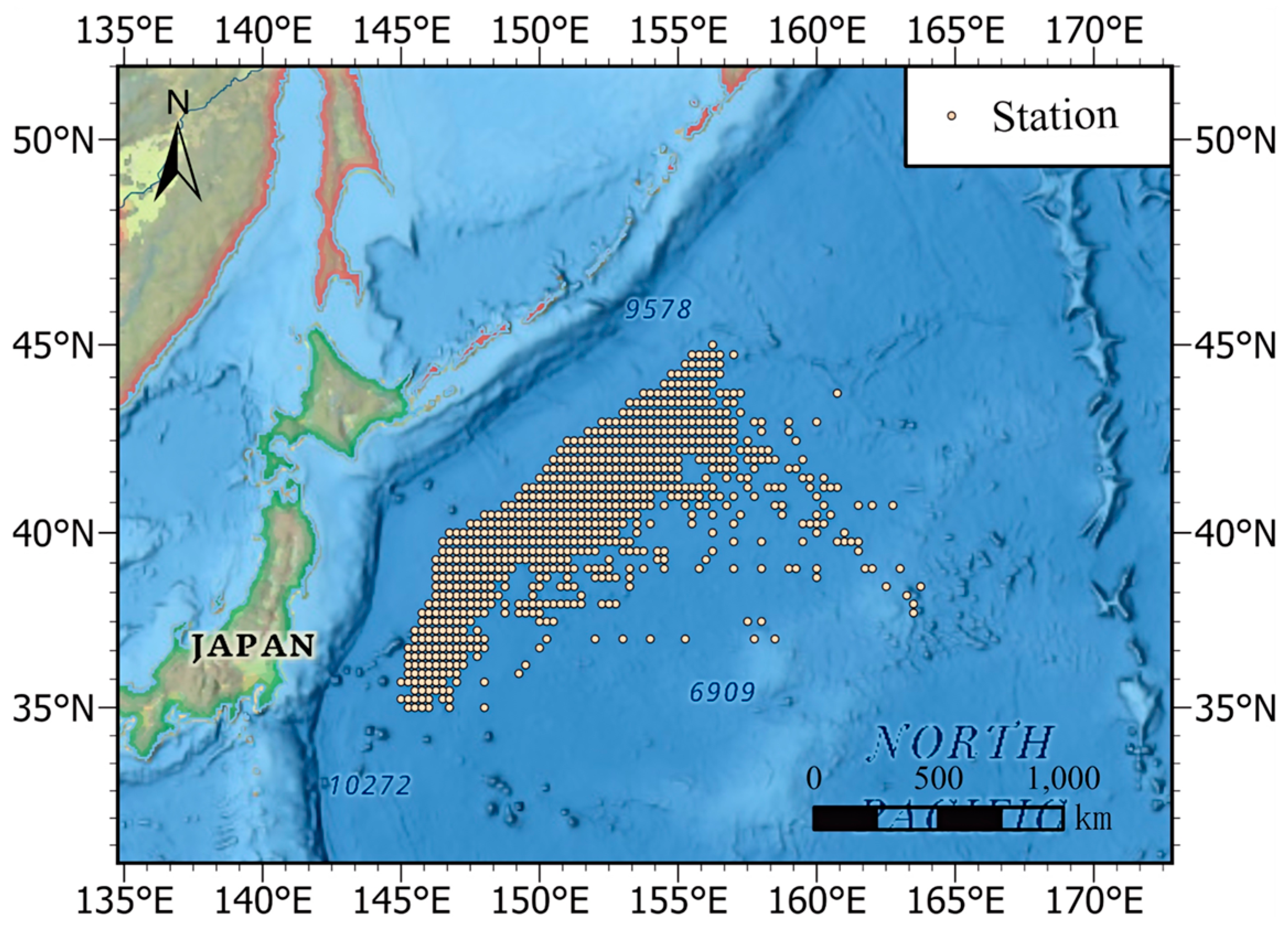
The fishery data for Chub Mackerel used in this study were obtained from the fishing logbooks of Chinese lighted purse seine vessels, covering the period from April to December during 2014–2022. The data are based on raw catch records, specifically the actual weight of Chub Mackerel caught by fishing vessels during their operations. The study area extends approximately between 145 and 163° E longitude and 35–45° N latitude, with fishing activities conducted in the high seas of the Northwest Pacific Ocean, as illustrated in
Figure 1. The dataset comprises 70,147 fishing records. These records include the catch amount for each fishing operation, the operation time, latitude and longitude information, as well as the corresponding environmental variables. The temporal resolution is daily, and the spatial resolution is 0.25° × 0.25°.
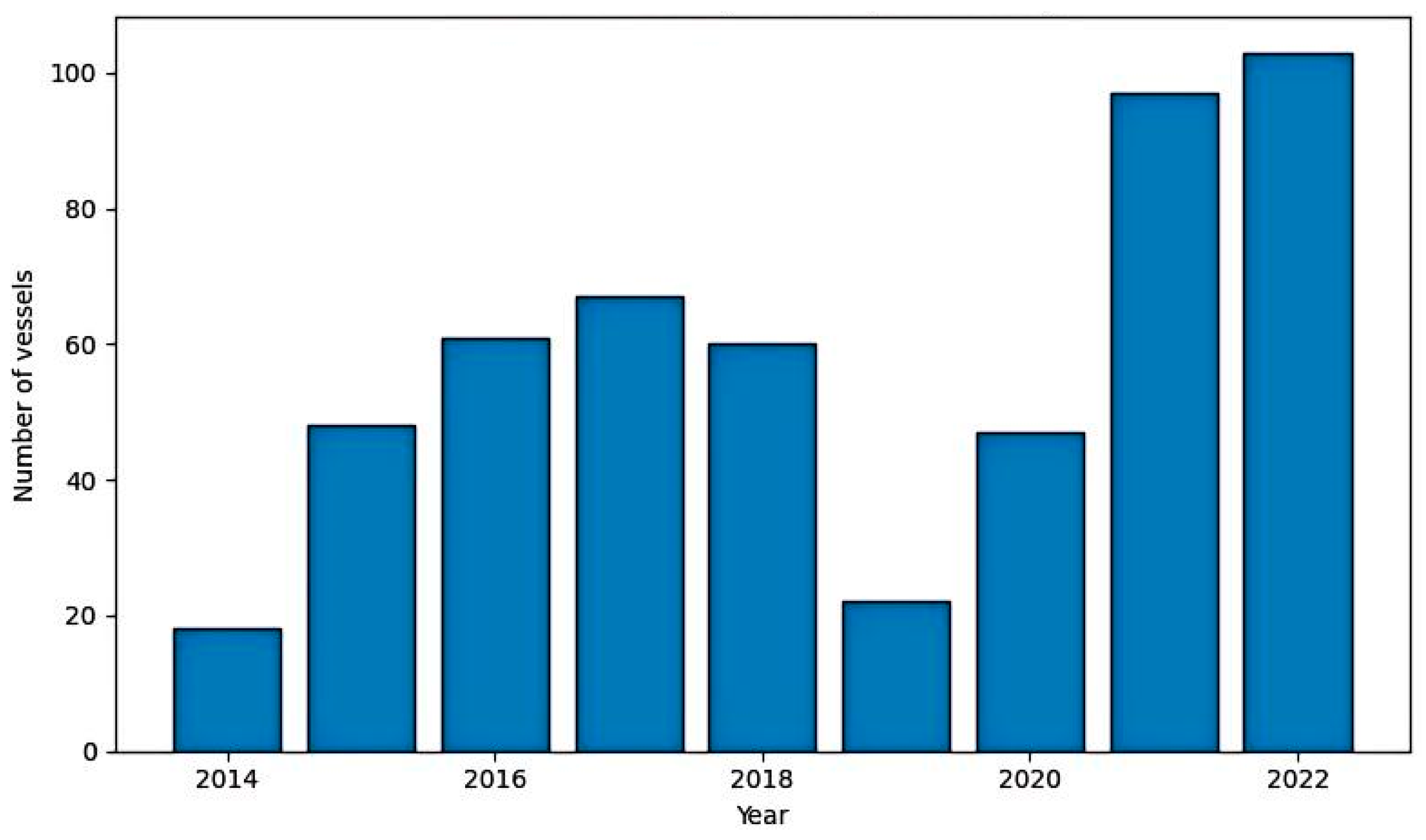
Figure 2 illustrates the variation in the number of Chinese lighted purse seine vessels from 2014 to 2022. Overall, the number of vessels exhibits a pattern of initial increase followed by fluctuations. Vessel numbers increased rapidly during 2014–2017, declined markedly in 2018–2019, and then rose again from 2020 onward. This temporal pattern directly reflects the stage-dependent fluctuations in fishing intensity over the study period.
Marine environmental variables were obtained from the Copernicus Marine Service Platform (
https://resources.marine.copernicus.eu/products, accessed on 3 May 2025). These data were extracted at the same temporal and spatial resolutions as the fishing logbooks and included sea surface temperature (SST), sea surface salinity (SSS), chlorophyll-a concentration (Chl-a), current velocity (CV), dissolved oxygen (DO), sea level anomaly (SLA), and mixed layer depth (MLD).
In particular,
is derived from the zonal (
) and meridional (
) geostrophic current velocities using the following formula. These two velocity components represent the flow speed along the latitude and longitude directions, respectively. By combining the velocity components from both directions, CV provides a simplified parameter that describes the overall intensity of water flow, suitable for ocean circulation studies and fishing ground distribution models. In research conducted on larger spatial scales, this combined approach helps simplify the model and enhances its practical applicability, while avoiding excessive refinement of directional flow velocities. This makes the results more concise and easier to interpret.
This study adopts a binary classification approach by calculating the median value of daily catch. Fishing areas with daily catches equal to or exceeding this median are defined as “high-abundance fishing grounds,” while the remaining areas are classified as “low-abundance fishing grounds.” In our dataset, the number of high-abundance samples is 35,075, and the number of low-abundance samples is 35,072, indicating a nearly balanced distribution between the two categories. To comprehensively evaluate model performance, multiple commonly used metrics were calculated, among which the F1-score, integrating both precision and recall, was selected as an important evaluation metric.
2.2. Data Types
For spatiotemporal variables, year, month, and latitude/longitude were selected as the basic indicators to analyze changes in the distribution of fishing grounds, thereby reflecting the temporal evolution and spatial characteristics of Chub Mackerel fishing grounds. For environmental variables, a set of physical and biological factors closely associated with fishery formation was considered, including SST (°C), SSS (‰), Chl-a (mg/m3), CV (m/s), DO (mmol/m3), MLD (m), and SLA (m).
The results indicated that SST, Chl-a concentration, and SSS were the core environmental factors influencing the distribution of Chub Mackerel fisheries in the Northwest Pacific Ocean. Specifically, SST strongly affects feeding activity and migration pathways [
19]; Chl-a, as an indicator of phytoplankton biomass, is associated with primary productivity and influences the availability of zooplankton and small pelagic prey, thereby indirectly affecting the distribution of Chub Mackerel [
20,
21,
22] and SSS represents water mass structure, exerting a regulatory effect on the stability of fish habitats [
23].
Although relatively few studies have examined the impacts of CV, DO, and MLD on Chub Mackerel fisheries, the literature suggests that these variables may play a significant role in regulating fish behavior and ecosystem processes.
DO [
24] concentration directly influences respiratory metabolism and vertical habitat selection; hypoxic zones may constrain the spatial range available to fish. CV [
25] not only provides the physical basis for migratory movements but also significantly affects the spatial distribution and aggregation of zooplankton, may influence fish feeding behavior. Interannual fluctuations in MLD [
26] regulate the efficiency of nutrient upwelling, which in turn impacts primary productivity in the upper water column and the survival conditions and recruitment success of migratory fish larvae.
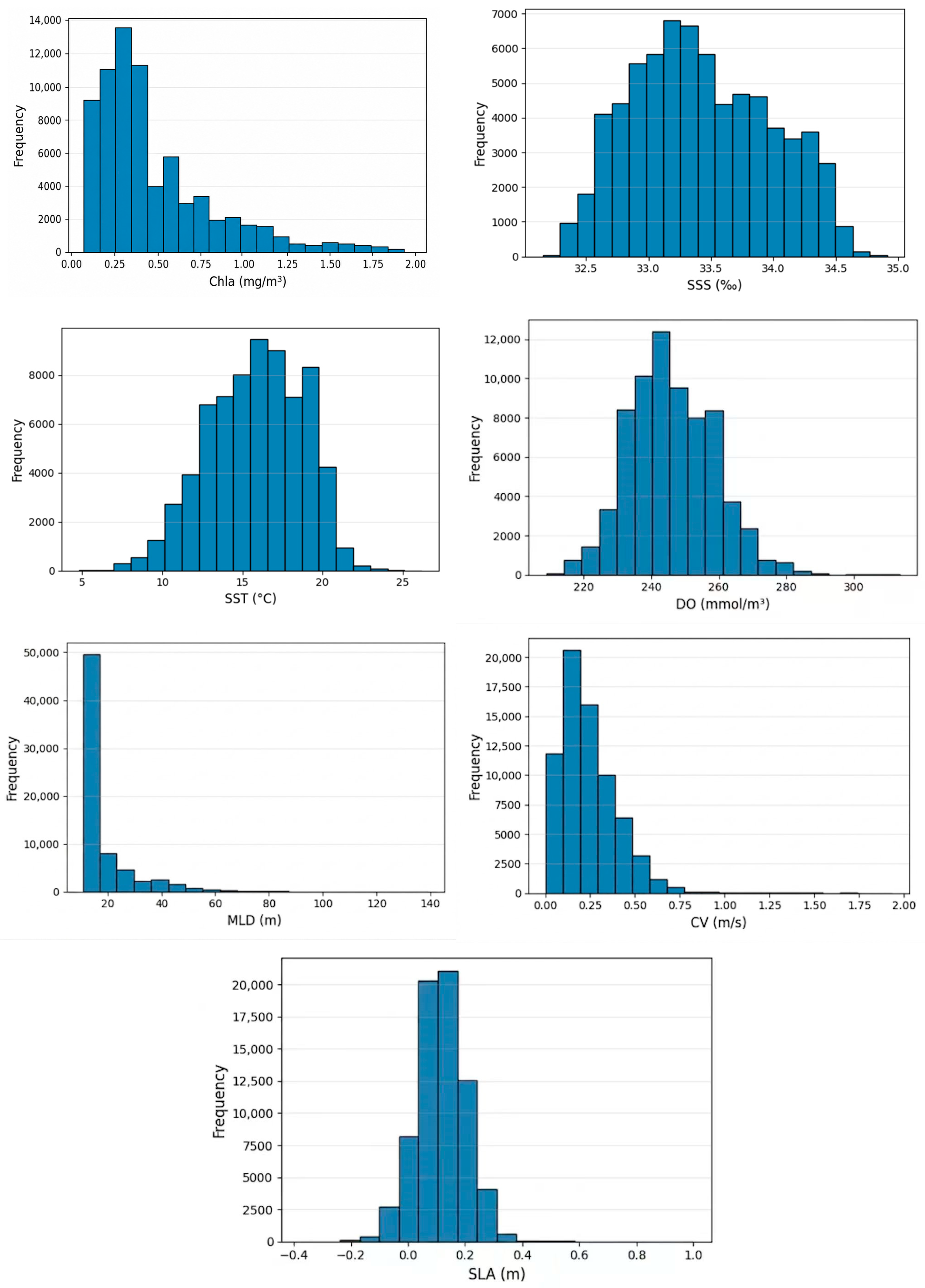
Figure 3 presents the histograms of potential marine environmental factors, while
Table 1 summarizes their basic statistics (mean, minimum, maximum, and skewness).
2.3. Normalization Process
To eliminate the influence of different measurement scales among environmental variables, all continuous variables were normalized prior to model construction. In this study, Min–Max normalization was applied to rescale the original data to the range of 0–1. The transformation can be expressed as:
where
represents the normalized value, and
denotes the original value of the variables, including fishing catch and environmental variables.
and
denote the minimum and maximum values of the corresponding variable, respectively. The environmental variables employed in this study exhibit considerable variation in their numerical ranges. Applying standardization is therefore crucial to alleviate potential biases introduced by these scale differences and to enhance the stability and overall performance of the machine learning models.
2.4. Machine Learning Algorithms
All machine learning models were implemented in Python version 3.10. In this study, four widely used machine learning models were selected: XGBoost (xgboost v3.1.3), LightGBM (lightgbm v4.6.0), RF (scikit-learn v1.7.2), and CatBoost (catboost v1.2.8).These models represent the most commonly applied ensemble learning approaches in structured data modeling. RF, proposed by Breiman in 2001, is based on bagging and random feature selection, offering stability and ease of use [
27]. XGBoost, officially released in 2016, has gained popularity in data science competitions due to its sparsity awareness, efficient regularization, and parallelization capabilities [
28]. LightGBM, also introduced in 2016 by Microsoft, is a gradient boosting decision tree (GBDT) framework that employs a leaf-wise growth strategy along with techniques such as Gradient-based One-Side Sampling (GOSS) and Exclusive Feature Bundling (EFB), making it particularly suitable for large-scale data processing. CatBoost, developed by Yandex in 2017, emphasizes efficient encoding of categorical features and mitigates the risk of information leakage [
29]. Collectively, these models are widely applied in domains such as financial risk control, recommender systems, click-through rate (CTR) estimation, and healthcare, and are considered indispensable benchmark methods in contemporary machine learning practice.
2.5. SHAP Interpretation Methods
SHapley Additive exPlanations (SHAP) has emerged as an important method for interpreting machine learning models [
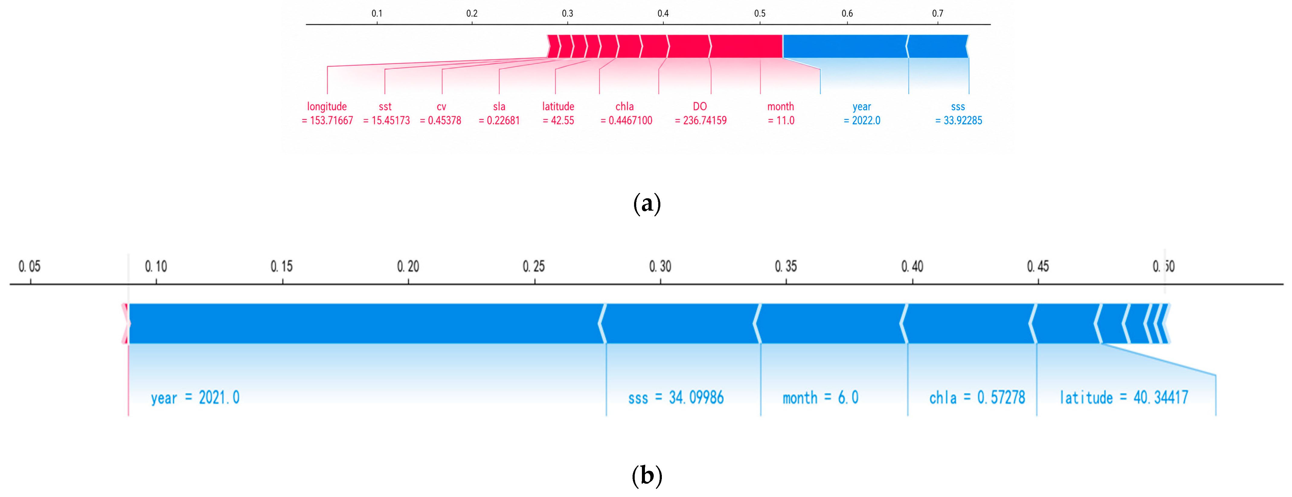
30], particularly tree-based models such as XGBoost, LightGBM, RF, and CatBoost, since its introduction in 2017. In this study, SHAP analysis was implemented using the Python package shap v0.44.1. It is grounded in the Shapley value from game theory and is characterized by theoretical fairness and local accuracy. Through the TreeSHAP and FastTreeSHAP algorithms, SHAP enables efficient interpretation of complex tree models, providing clear explanations of single-sample prediction processes while also revealing global feature importance and feature interactions. In practice, SHAP not only enhances model interpretability but is also widely applied in feature selection and model optimization, making it a cornerstone of explainable AI. The core formulation of SHAP is derived from the Shapley value equation in game theory, which quantifies the “average marginal contribution” of each feature to the model output. For a model f, the SHAP value of feature i is defined as follows.
where
N denotes the set of all features;
S denotes any subset that does not contain feature
i;
denotes the number of features in subset
S;
represents the model prediction using only the feature subset
S.
denotes the SHAP value of feature
i, its average marginal contribution to the model output.
2.6. Variable Selection and Predictive Performance Evaluation
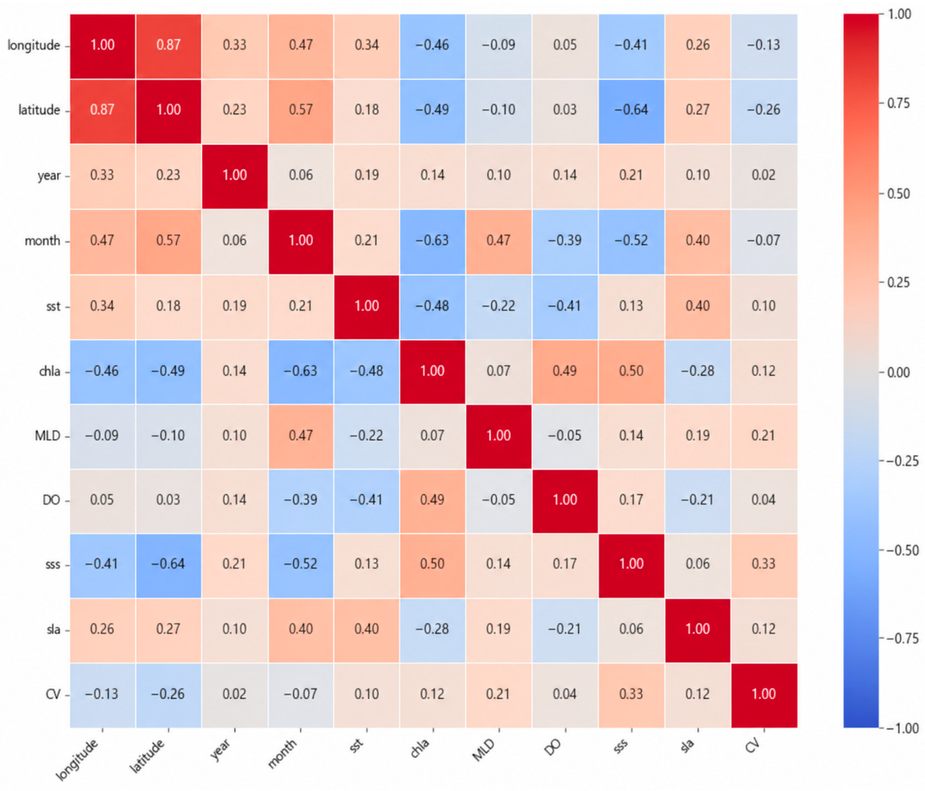
Feature selection is a critical step in machine learning, as it helps reduce training time, decrease model complexity, and enhance prediction performance. A Pearson correlation coefficient close to ±1 suggests potential redundancy between variables, which may diminish the effective contribution of certain variables during model training [
31]. In this study, Pearson correlation coefficients were calculated among all variables, as shown in
Figure 4. The results indicate generally weak correlations between most variables, with a maximum absolute value not exceeding 0.87, which is below the common collinearity exclusion threshold of 0.9.
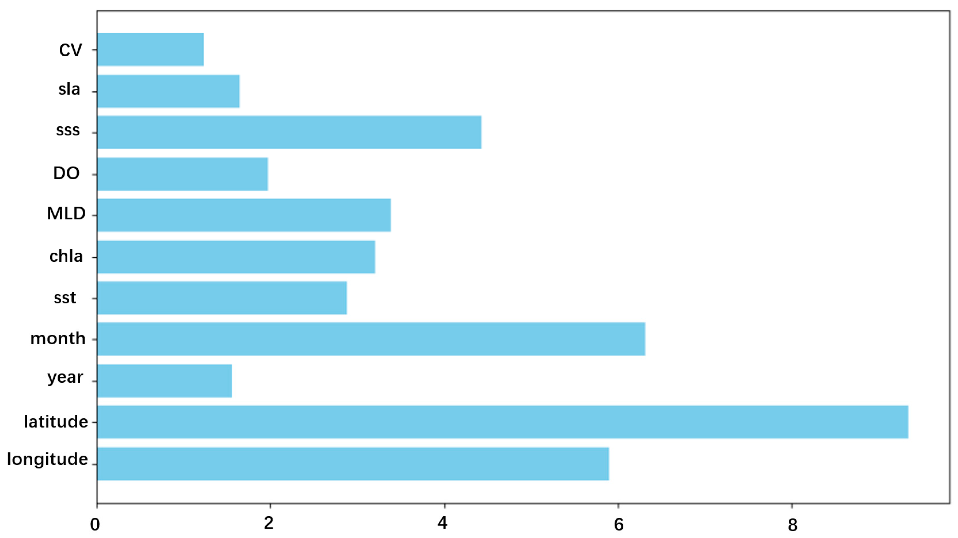
The variance inflation factor (VIF) is a key method for detecting multicollinearity among variables, quantifying the extent to which the variance of a variable is inflated due to its linear dependence on other predictors, and is regarded as a robust metric for assessing collinearity in regression models. The VIF values of the variables are shown in
Figure 5. Specifically, the VIF values for latitude, longitude, and month are 9.3, 5.9, and 6.2, respectively.
Referring to the study [
32], which advises caution regarding rigid rules of thumb for VIF thresholds, although the VIF values for month, longitude, and latitude are relatively high, they are all below 10, indicating no severe multicollinearity. Moreover, these three variables represent important spatiotemporal factors influencing the distribution of Chub Mackerel (
Scomber japonicus) fishing grounds and are therefore retained in the modeling process. The VIF values for other environmental variables are all relatively low, confirming their suitability for inclusion in subsequent model construction.
The dataset was divided into a training set (70%) and a testing set (30%) using a stratified random splitting approach, ensuring that the proportions of the “high-abundance” and “low-abundance” classes in both subsets remained consistent with those in the original dataset, thereby avoiding potential biases in model training and evaluation caused by class imbalance.
In binary classification tasks such as fishing ground prediction, model performance is commonly assessed using four basic statistics derived from the confusion matrix: true positives (TP), false positives (FP), true negatives (TN), and false negatives (FN) [
33]. These values are then used to calculate key performance metrics, including accuracy, precision, recall, and the F1-score, which are essential for model tuning and result interpretation.
Among them, TP represents the number of samples correctly predicted by the model to be in the positive category; TN represents the number of samples correctly predicted by the model to be in the negative category; FP represents the number of samples incorrectly predicted by the model to be in the positive category; and FN represents the number of samples incorrectly predicted by the model to be in the negative category. Accuracy represents the proportion of overall correct predictions made by the model; precision reflects how many of the classes predicted as positive are truly positive; recall measures the ability of the model to identify all samples in the positive class; and the F1-score is the harmonic mean of precision and recall, which is used to comprehensively evaluate the performance of the model on imbalanced datasets. Additionally, to examine the trend variations in annual and monthly production, we conducted the Mann–Kendall trend test. This method is a non-parametric statistical approach used to detect monotonic trends (either increasing or decreasing) in time series data. The test was performed using the “Kendall” package in R software (version 4.0.3).
4. Discussion
4.1. Analysis of Changes in Chub Mackerel Catch from 2014 to 2022
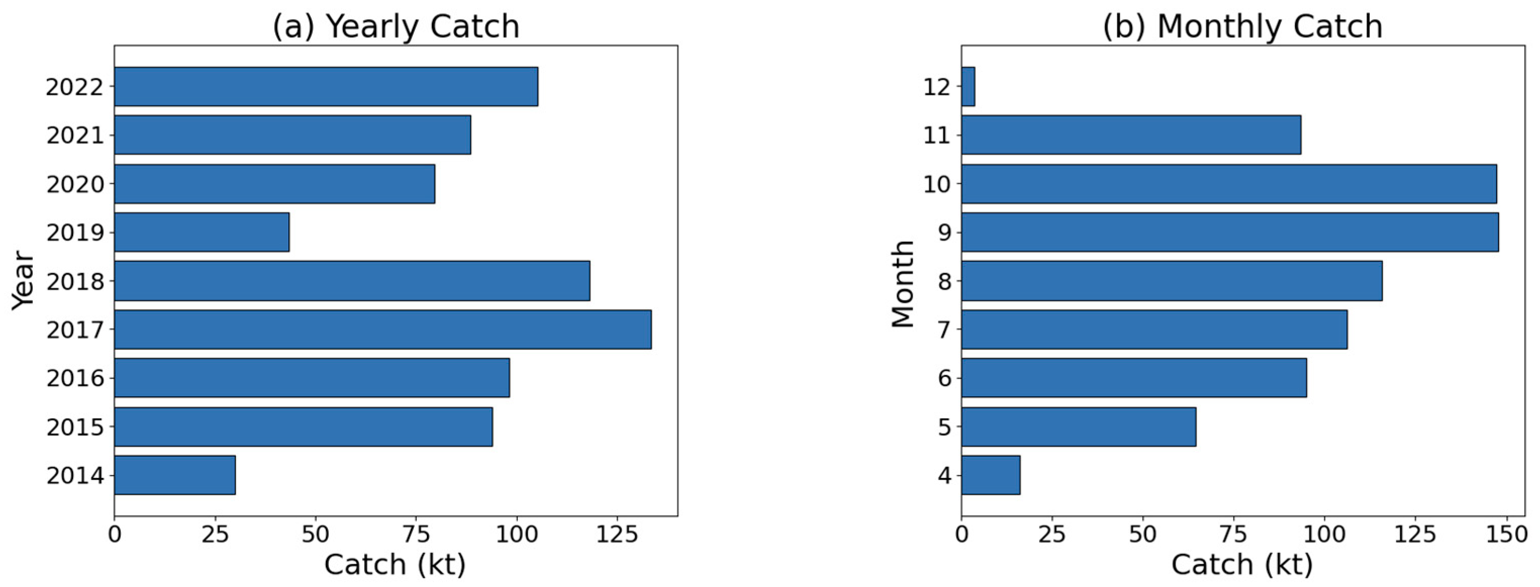
The interannual fluctuations in Chub Mackerel catches between 2014 and 2022 exhibit complex, multifactorial trends. Resource dynamics during this period were reflected not only in quantitative increases and decreases but also in deeper changes in ecosystem structure and fishery practices. Several factors may explain these variations: (1) shifts in the marine environment under global warming, particularly rising seawater temperatures and changes in the position of the Kuroshio Extension, significantly influenced habitat selection and spawning ground distribution, leading to regional redistribution and aggregation of stocks [
34]; (2) Food competition and density effects between Japanese sardine and Chub Mackerel substantially impact the population dynamics of Chub Mackerel. An increase in sardine abundance may reduce food availability for Chub Mackerel, thereby affecting their growth and catch levels [
35]. (3) The high catch levels in the high seas of the Northwest Pacific are closely linked to high fishing intensity, which may be one of the factors contributing to the sharp decline in catches in 2019 [
36].
Regarding intermonthly fluctuations, the study confirmed that Chub Mackerel aggregated in the southwestern Sea of Japan from October to December before migrating southward to the East China Sea and adjacent offshore waters for wintering. The SST ranges and optimal intervals for Chub Mackerel fishing grounds differ between spring and summer. In spring, fishing grounds are found within an SST range of 7–19 °C, with an optimal SST of 11–15 °C. In summer, the SST range is 8–24 °C, with an optimal SST of 8–12 °C. This demonstrates a clear seasonal preference for specific temperature conditions [
37].
In other regions, Atlantic mackerel (
Scomber scombrus) also exhibits a significant preference for the thermocline and specific temperature ranges (8–12 °C), particularly during the colder seasons, when they adjust their habitat distribution in response to changes in the thermocline [
38]. This behavior is similar to the monthly fluctuations observed in Chub Mackerel (
Scomber japonicus) in the Northwest Pacific. The fishing grounds of Chub Mackerel in the Northwest Pacific Ocean are extensive, mainly concentrated between 39 and 43° N latitude and 149–154° E longitude. Key fishing areas include the high seas east of Honshu, the eastern coast of Japan, the northern East China Sea, the eastern edge of the Yellow Sea, and the Russian Far East [
39], consistent with the findings of this study.
In summary, the spatial and temporal dynamics of Chub Mackerel catches reveal pronounced interannual and intermonthly variability. These findings provide an ecological basis for stock assessment and fishery management, emphasizing that fishery strategies should be more closely aligned with the natural migratory rhythms of the stock and the broader context of climate change.
4.2. Prediction Performance Analysis of Four Machine Learning Models
The applications of XGBoost, LightGBM, CatBoost, and RF in environmental prediction have grown steadily, demonstrating excellent modeling performance, particularly in nonlinear, multivariate systems where they show clear advantages. In fisheries, Han et al. [
12] applied RF and LightGBM to operational and environmental data from 2014 to 2022 and achieved a prediction accuracy of approximately 75%. They further noted that variable importance changed significantly under different light conditions, suggesting that environmental factors such as sea surface height anomaly, salinity, and dissolved oxygen play key roles in determining fishing ground distribution.
Further research has also confirmed this, several studies have consistently shown that Chl-a, SSS, DO, and SST are the primary factors influencing fishery distribution in machine learning-based prediction models. Zhang et al. [
40], for example, found that Chl-a was the most critical factor in January, while latitude exerted the strongest influence in year-round predictions of albacore tuna fisheries in the South Pacific Ocean using a RF model for feature importance analysis. Fang et al. [
41] in a study of squid fisheries of Chile using the HSI model, reported that the combination of SST and SSS outperformed other variable configurations in predictive accuracy. Similarly, Zhang et al. [
42] employed LightGBM and CatBoost in combination with SHAP interpretation to evaluate environmental variable importance in predicting Atlantic albacore tuna fisheries. Their results indicated that temperature and dissolved oxygen at a depth of 100 m were the most influential variables across multiple spatial scales, with SSS playing a secondary role.
Overall, while species-specific ecological traits and regional characteristics affect the ranking of variable importance, Chl-a, SSS, DO, and SST consistently emerge as the core environmental parameters for constructing high-performance fishery prediction models. Our results are broadly consistent with previous findings, and we emphasize that careful selection of optimal hyperparameters and appropriate normalization of environmental variables are essential when building such models.
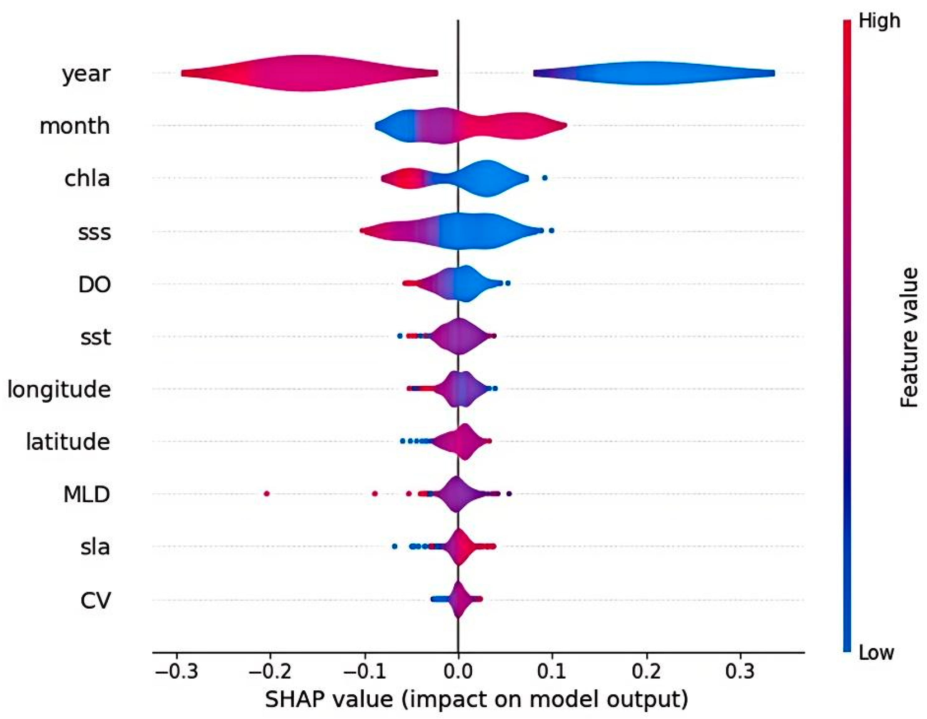
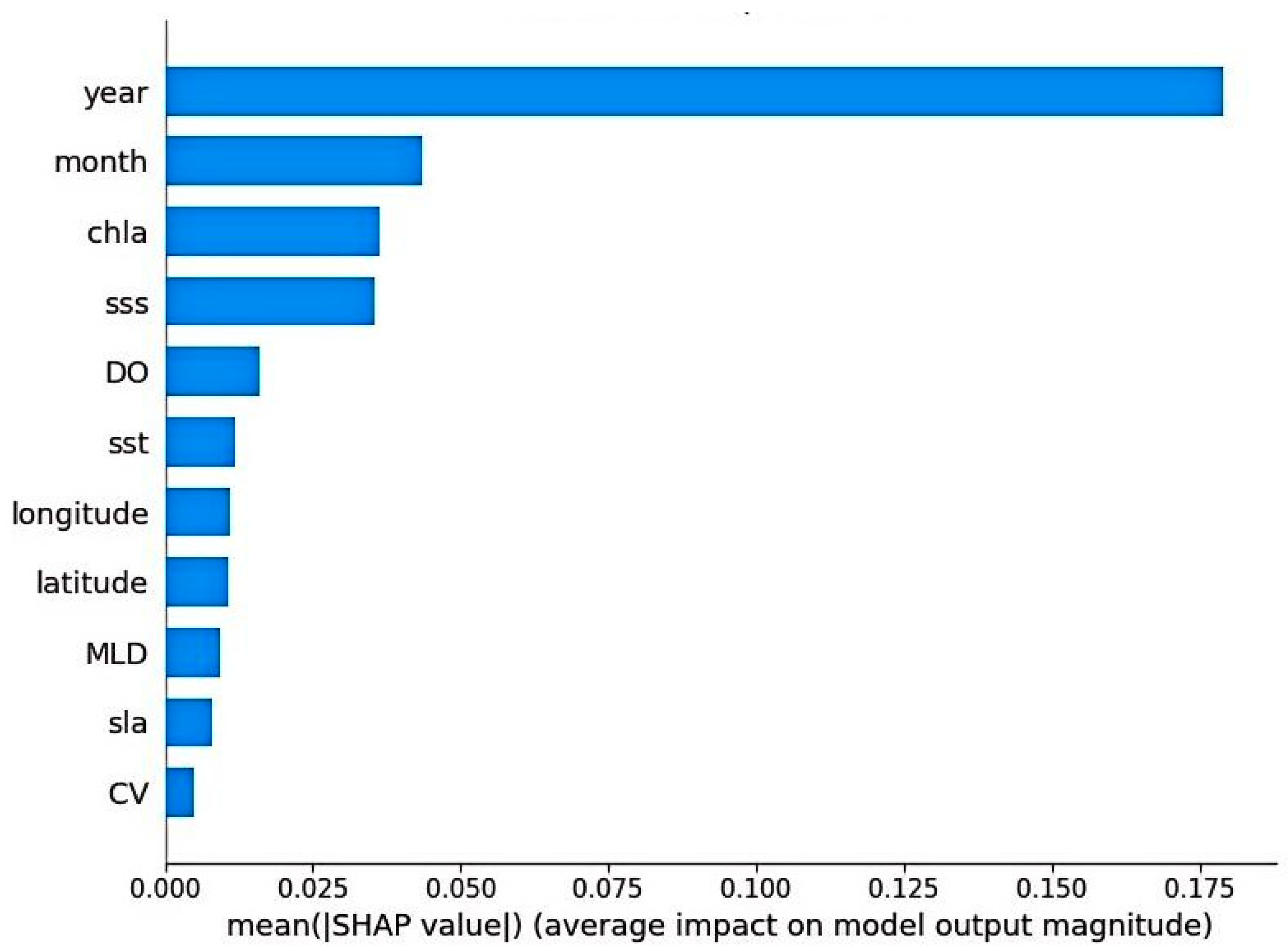
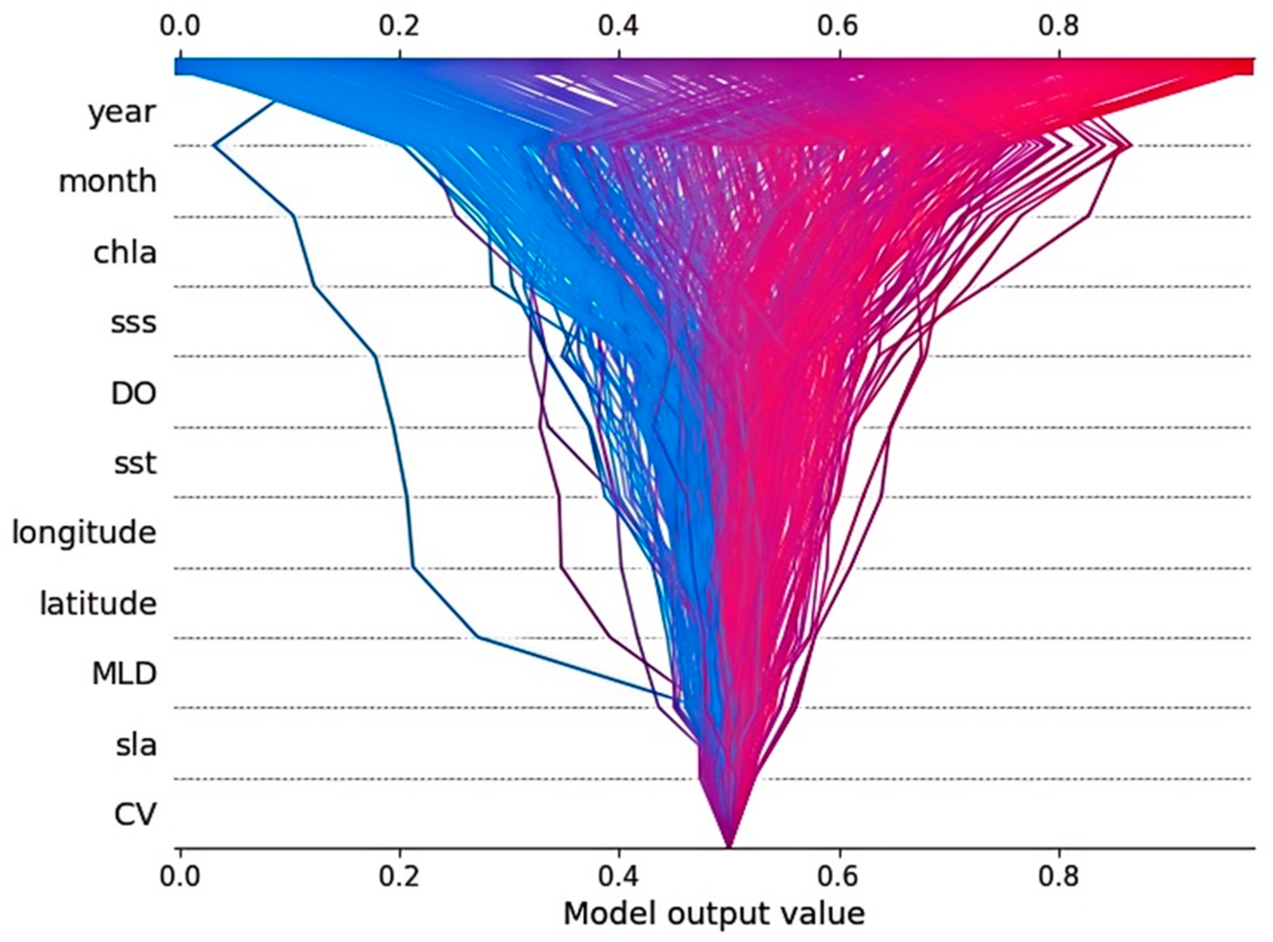
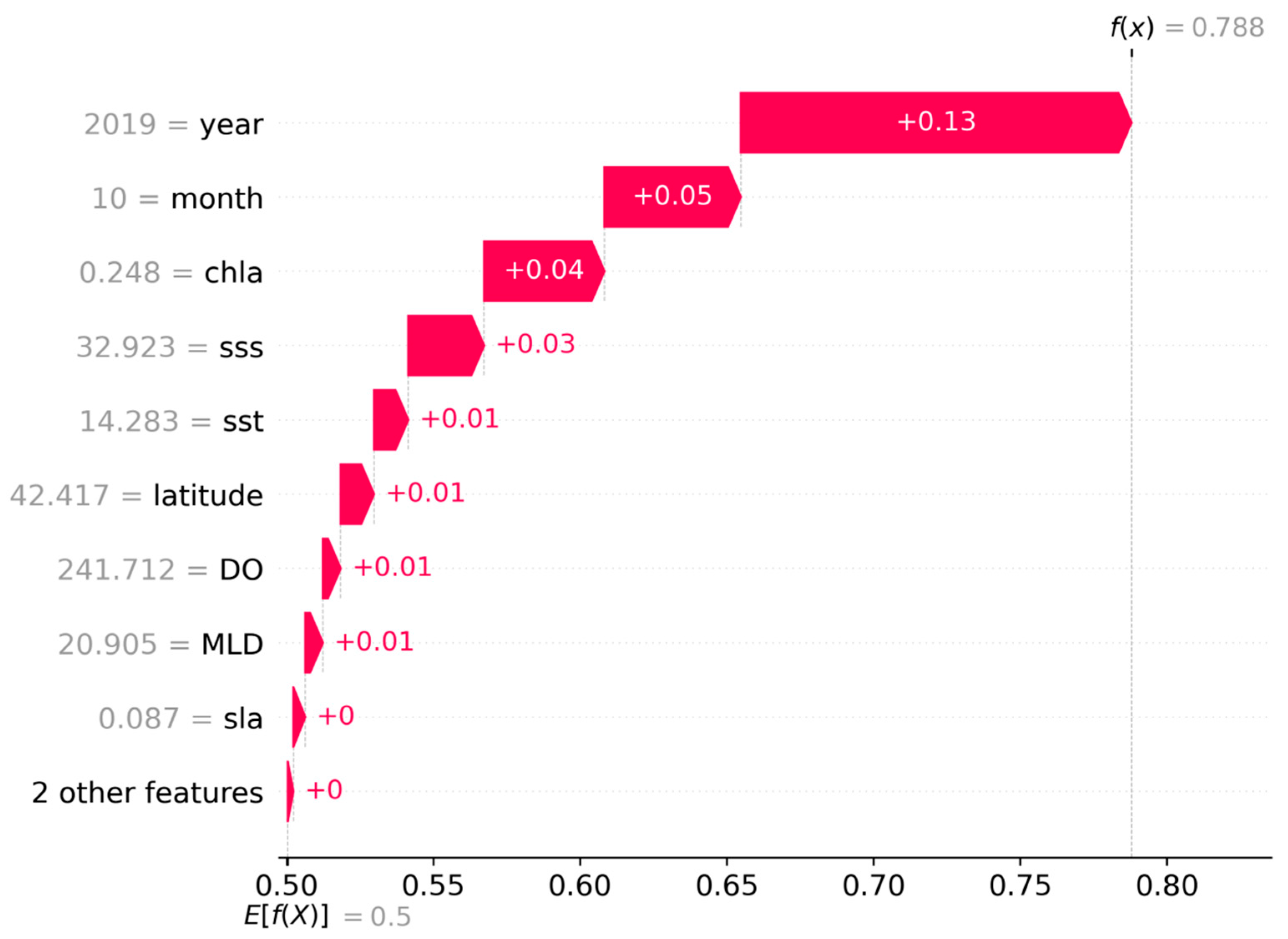
The results of this study indicate that the importance of the “year” and “month” variables is higher than that of other marine environmental factors. This is primarily because interannual variations are mainly driven by the stages of fishery development and management policies. The light purse seine fishery in the Northwest Pacific of China began to develop in 2014, with limited fishing vessel scale and immature technology during the early stages, resulting in lower production. As the scale of operations expanded, production increased annually. By 2019, production experienced a temporary downturn due to industrial restructuring; however, following adaptive adjustments in the industry and the resource management measures implemented by the North Pacific Fisheries Management Organization (NPFC), production gradually increased and stabilized at around 100,000 tons. On a monthly scale, Chub Mackerel, as a typical seasonal migratory species, has a significantly concentrated fishing season, primarily from June to November, resulting in noticeable fluctuations in monthly production. These factors led to significant variations in Chub Mackerel production across years and months, directly influencing its SHAP values in the model.
However, this study has several limitations: (1) the catch data used were derived from existing fishery statistics, which did not cover all potential fishing areas and thus introduced spatial gaps; (2) although the input variables encompassed a broad range of marine environmental parameters, they did not include dynamic elements such as currents, cyclonic activity, ocean front positions, or extreme meteorological events, which may strongly influence fishing ground distribution at specific spatial and temporal scales; (3) socio-economic factors—including changes in fishing behavior, policy adjustments, and the intensity of fishing vessel operations—were not sufficiently considered, which may introduce prediction bias. (4) While this study has employed the SHAP method for interpretation, it has not explicitly captured the potential interactions among environmental factors (such as the synergistic effect between SST and Chl-a), nor has it quantitatively assessed prediction uncertainty, which to some extent limits the depth of ecological interpretation. Future research should integrate multi-source environmental dynamics and socioeconomic drivers, incorporating interaction features, uncertainty quantification methods, and additional dynamic environmental elements to enhance the accuracy and practical applicability of fishery prediction models.
4.3. Recommendations for the Management of the Chub Mackerel Fishery in the Northwest Pacific Ocean
Chub Mackerel is one of the most economically valuable migratory pelagic fish species in the Northwest Pacific, and its catch plays an important role in the fisheries sectors of several coastal countries. Owing to its extensive migratory behavior and highly sensitive ecological traits, the population dynamics of this species are not only directly influenced by fishing intensity but also shaped by complex environmental factors such as variations in ocean temperature, salinity, and currents, all of which exhibit strong spatiotemporal variability. Therefore, establishing a scientific, systematic, and adaptive management framework is of great practical importance to ensure the sustainable development of Chub Mackerel resources.
To achieve effective management of this species, a systematic governance framework should be developed at multiple levels, encompassing fishing control, resource assessment and optimization, and regional cooperation mechanisms. Firstly, given the significant spatial and temporal differences in population distribution, differentiated quota strategies should be implemented based on seasons and geographical locations. Seasonal fishing bans or total allowable catch (TAC) limits should be enforced in high-density areas. At the same time, fishing intensity and vessel capacity should be strictly controlled to reduce the risk of overfishing. Secondly, to enhance the adaptability and foresight of management, key environmental factors such as sea temperature, salinity, and mixed-layer depth should be incorporated into the resource assessment framework, thereby promoting an ecosystem-coupled management approach. By systematically integrating high-resolution oceanographic variables, satellite environmental indices, and fleet behavior data, model prediction accuracy can be effectively improved, providing more reliable scientific support for fisheries resource management. Thirdly, full use should be made of the NPFC and its technical working groups to regularly update resource status assessments, facilitate joint data collection, model evaluation, and policy consultations among member states, and advance the process of transnational cooperative governance. Collectively, these comprehensive measures are expected to ensure the long-term sustainable utilization of Chub Mackerel resources while maintaining the economic viability of the fishery.
5. Conclusions
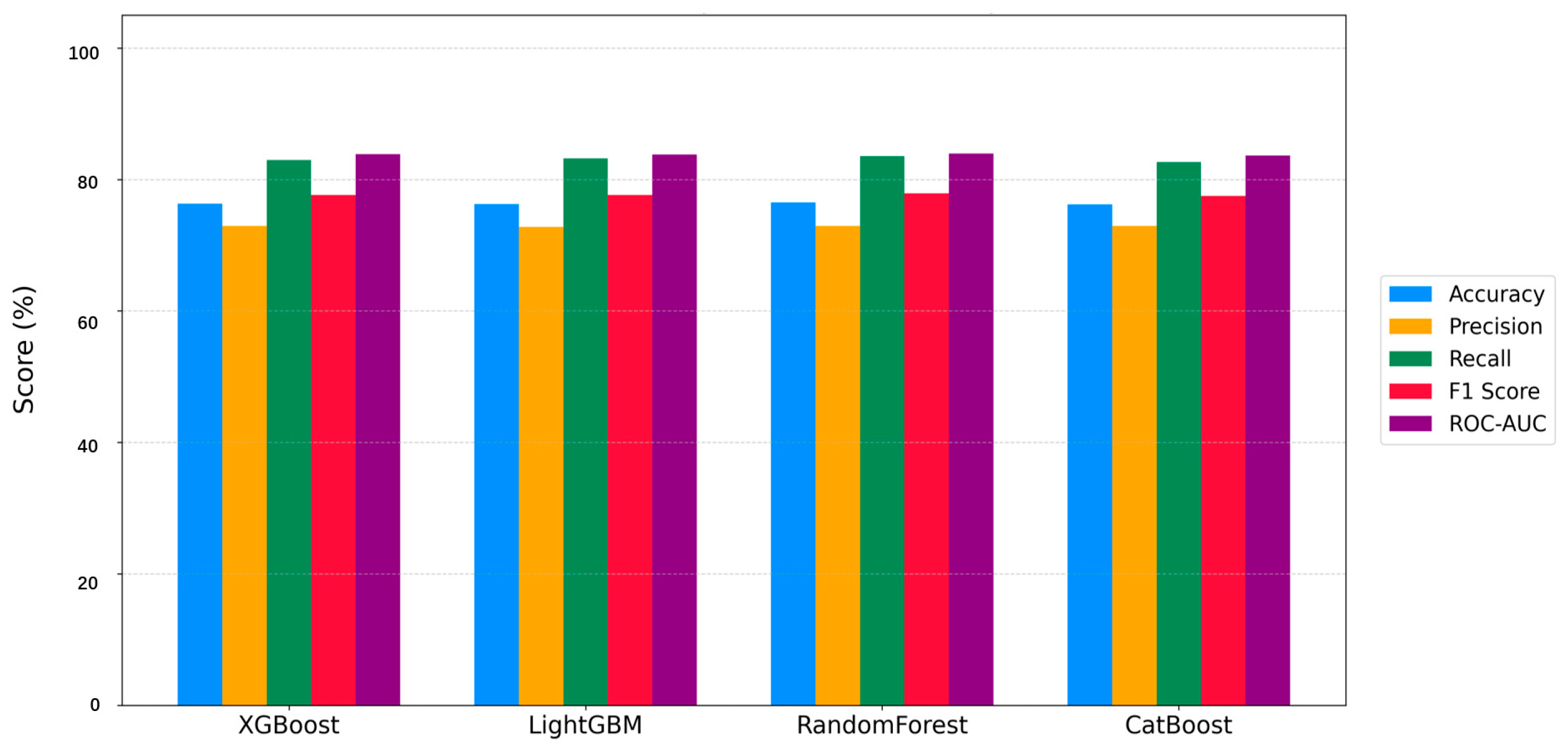
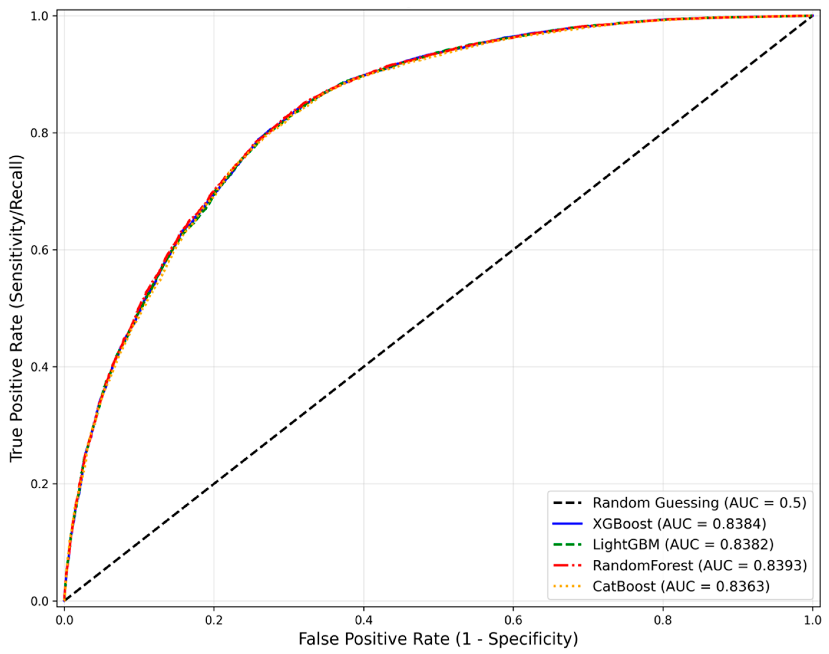
Based on the analysis of Chub Mackerel catch data in the Northwest Pacific from 2014 to 2022, this study reveals pronounced interannual fluctuations in catch volume, which reached the peak in 2017–2018 and significantly decreased in 2019. At the monthly scale, catches were concentrated from June to November, peaking in September–October. Among the four machine learning models evaluated, the RF model demonstrated the highest performance in predicting fishing ground distribution. Interpretability analysis based on the SHAP framework further indicated that temporal variables (year and month) contributed most significantly to the predictions, while environmental factors such as Chl-a, SSS, DO, and SST also played important roles.
While this study has yielded certain findings, it is not without limitations. The predictive performance of the model is, to some extent, contingent upon the type and quality of the input environmental variables. Certain potential critical factors (such as higher-resolution ocean dynamic processes) have yet to be incorporated into the analysis. Moreover, existing data still exhibit constraints in terms of temporal and spatial resolution, which may affect the model’s ability to accurately capture local-scale variations. Future research should integrate multi-source dynamic environmental data including ocean currents, mesoscale eddies, and oceanic fronts as well as socio-economic factors such as fisheries’ management policies and fishing vessel operation patterns, in order to construct a more robust and spatiotemporally adaptive prediction framework. Such an integrated modeling approach will provide more reliable scientific support for the sustainable management of fishery resources under climate change.