Author Contributions
Conceptualization, X.L. and L.H.; methodology, X.L.; validation, Q.L., R.W., B.L., Z.L., Y.S. and Z.H.; formal analysis, X.L.; investigation, X.L., L.H., Q.L., R.W., B.L., Z.L., Y.S. and Z.H.; resources, L.H.; data curation, X.L., Q.L., R.W., B.L., Z.L., Y.S. and Z.H.; writing—original draft preparation, X.L.; writing—review and editing, L.H.; visualization, X.L.; supervision, L.H.; project administration, L.H.; funding acquisition, L.H. All authors have read and agreed to the published version of the manuscript.
Figure 1.
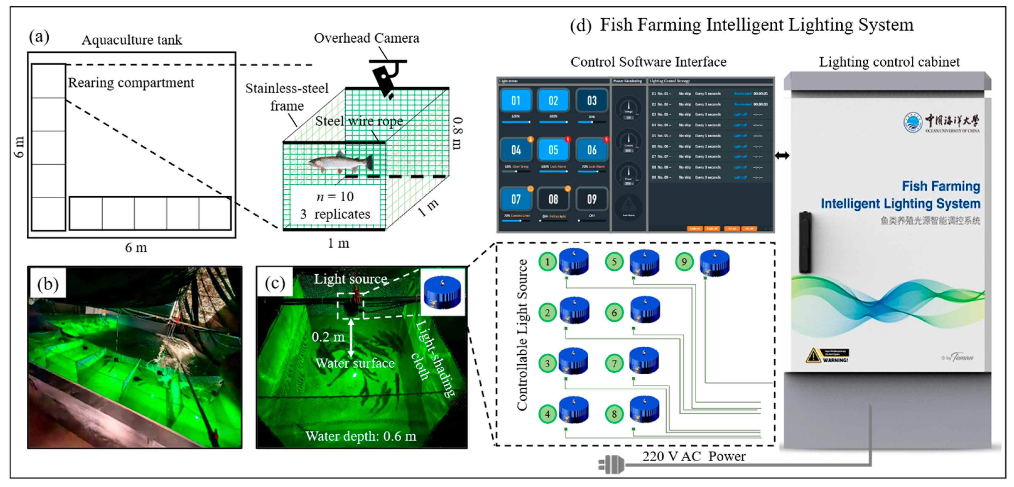
Schematic diagram of the experimental system. (a) Structure of the rearing compartments (1 m × 1 m× 0.80 m) installed in the aquaculture tank (6 m × 6 m) and the camera positioned above each compartment for behavioral recording; (b) overall layout of the experimental setup in the aquaculture tank; (c) arrangement of the controllable light source above the water surface (20 cm) and installation of light-shading cloth between adjacent compartments to prevent light interference among treatments; and (d) Fish Farming Intelligent Lighting System used to regulate light intensity and photoperiod, including the control software interface, lighting control cabinet, and controllable light sources. The schematic diagram was created using Microsoft PowerPoint (Microsoft Corp., Redmond, WA, USA).
Figure 1.
Schematic diagram of the experimental system. (a) Structure of the rearing compartments (1 m × 1 m× 0.80 m) installed in the aquaculture tank (6 m × 6 m) and the camera positioned above each compartment for behavioral recording; (b) overall layout of the experimental setup in the aquaculture tank; (c) arrangement of the controllable light source above the water surface (20 cm) and installation of light-shading cloth between adjacent compartments to prevent light interference among treatments; and (d) Fish Farming Intelligent Lighting System used to regulate light intensity and photoperiod, including the control software interface, lighting control cabinet, and controllable light sources. The schematic diagram was created using Microsoft PowerPoint (Microsoft Corp., Redmond, WA, USA).
Figure 2.
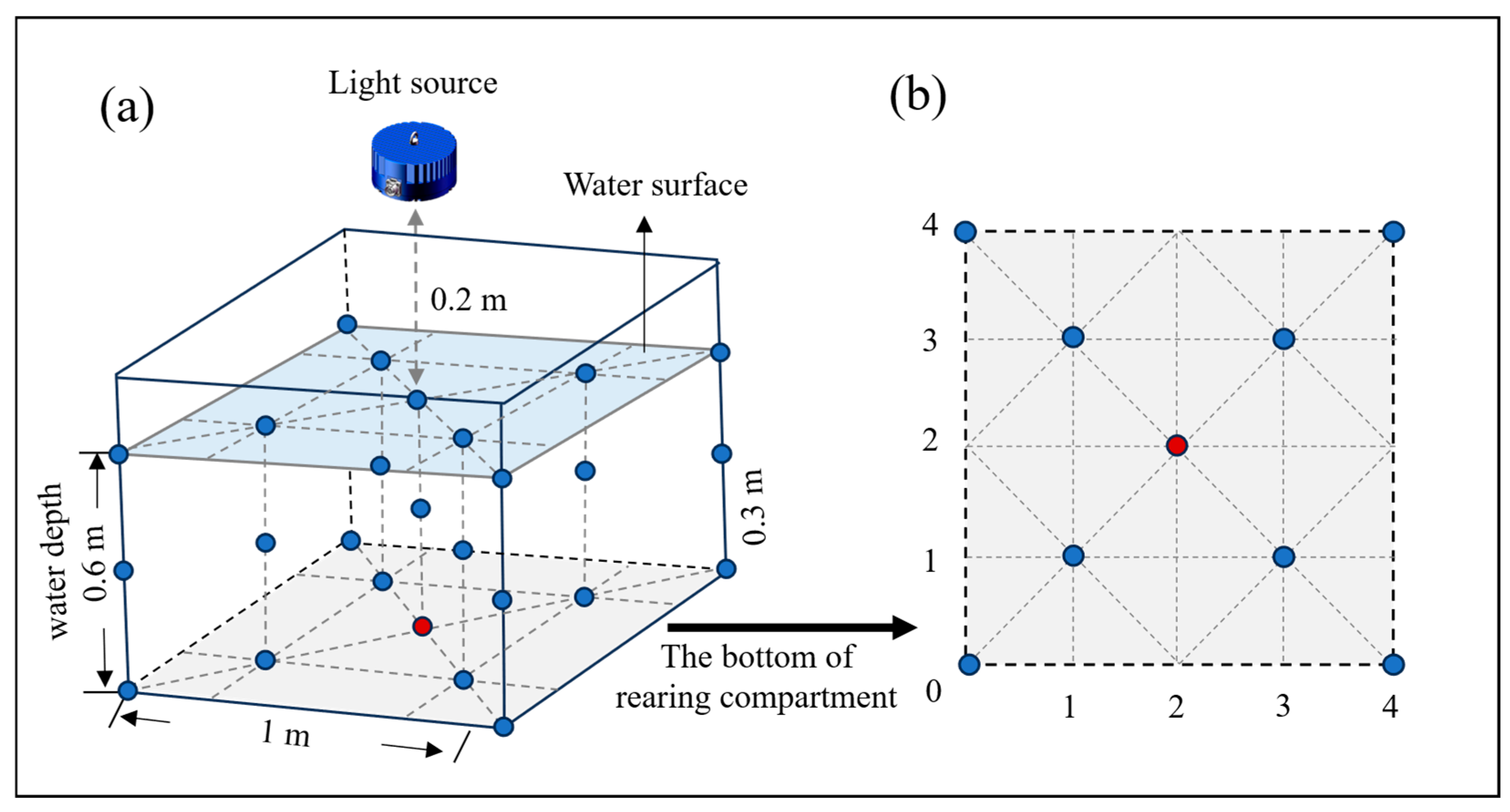
Schematic diagram of the illuminance measurement points. (a) Overall measurement points within the rearing compartment, and (b) measurement points at the compartment bottom. The solid blue and red dots represent the location of illuminance sensors in each rearing compartment. The red dot marks the center of the tank bottom, directly below the light source; the target illuminance for the experiment was calibrated based on the readings from this point.
Figure 2.
Schematic diagram of the illuminance measurement points. (a) Overall measurement points within the rearing compartment, and (b) measurement points at the compartment bottom. The solid blue and red dots represent the location of illuminance sensors in each rearing compartment. The red dot marks the center of the tank bottom, directly below the light source; the target illuminance for the experiment was calibrated based on the readings from this point.
Figure 3.
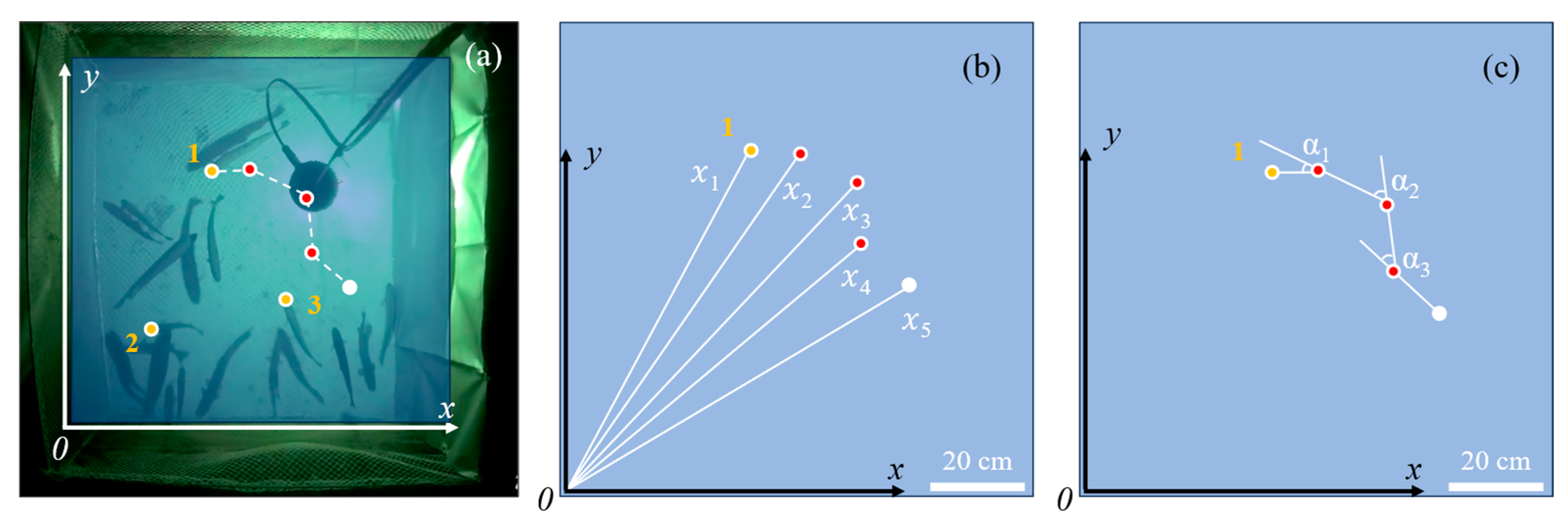
Swimming behavior tracking and calculation. (a) Orange dots mark three randomly selected experimental fish (No. 1–3), tracked by snout position. White dotted lines between red points show swimming trajectories between frames. White points are starting positions; orange points are endpoints. The distance between them is the total movement distance, TM. (b) Average distance of the fish snout points from the origin (.
(c) Average change in movement angle ().
Figure 3.
Swimming behavior tracking and calculation. (a) Orange dots mark three randomly selected experimental fish (No. 1–3), tracked by snout position. White dotted lines between red points show swimming trajectories between frames. White points are starting positions; orange points are endpoints. The distance between them is the total movement distance, TM. (b) Average distance of the fish snout points from the origin (.
(c) Average change in movement angle ().
Figure 4.
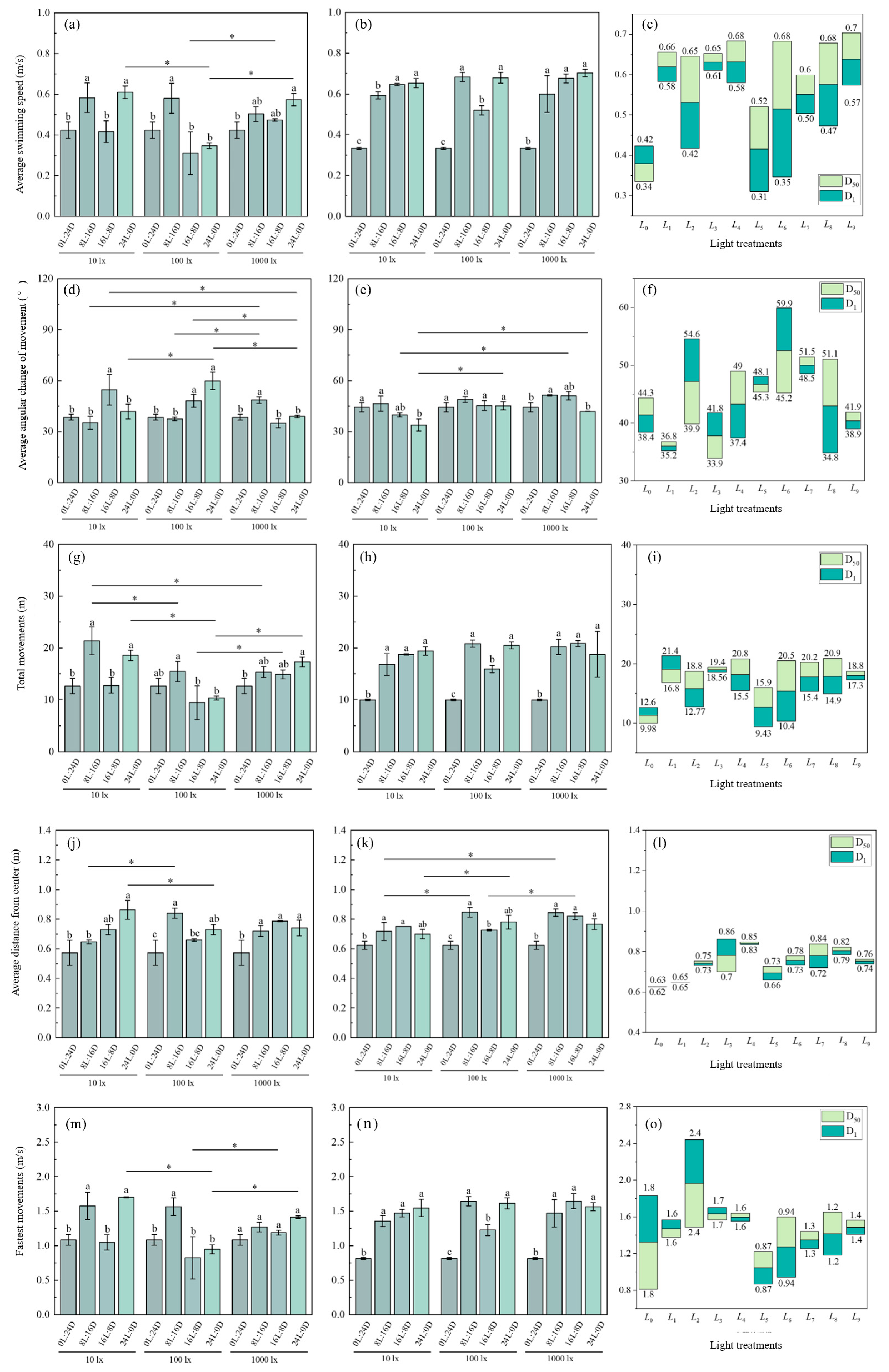
The effects of light intensity, photoperiod, and treatment duration on the swimming behavior parameters of rainbow trout. (a) AS, D1, (b) AS, D50, (c) AS, D1 vs. D50, (d) AC, D1, (e) AC, D50, (f) AC, D1 vs. D50, (g) TM, D1, (h) TM, D50, (i) TM, D1 vs. D50, (j) DC, D1, (k) DC, D50, (l) DC, D1 vs. D50, (m) FM, D1, (n) FM, D50, and (o) FM, D1 vs. D50. Different lowercase indicates significant differences between treatment groups of different photoperiods under the same light intensity (p < 0.05), and * indicates significant differences between treatment groups of different light intensities within the same photoperiod (p < 0.05).
Figure 4.
The effects of light intensity, photoperiod, and treatment duration on the swimming behavior parameters of rainbow trout. (a) AS, D1, (b) AS, D50, (c) AS, D1 vs. D50, (d) AC, D1, (e) AC, D50, (f) AC, D1 vs. D50, (g) TM, D1, (h) TM, D50, (i) TM, D1 vs. D50, (j) DC, D1, (k) DC, D50, (l) DC, D1 vs. D50, (m) FM, D1, (n) FM, D50, and (o) FM, D1 vs. D50. Different lowercase indicates significant differences between treatment groups of different photoperiods under the same light intensity (p < 0.05), and * indicates significant differences between treatment groups of different light intensities within the same photoperiod (p < 0.05).
Figure 5.
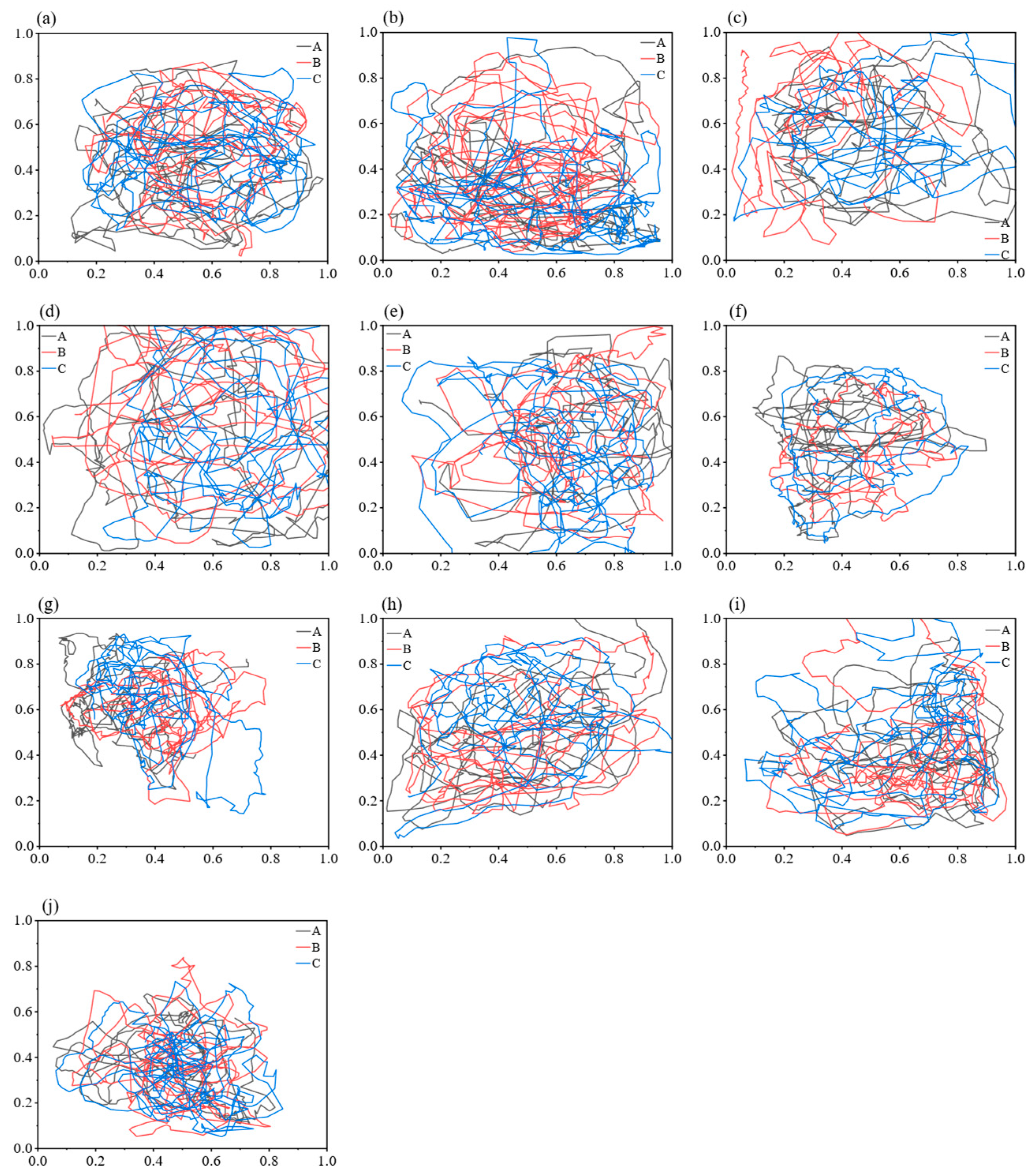
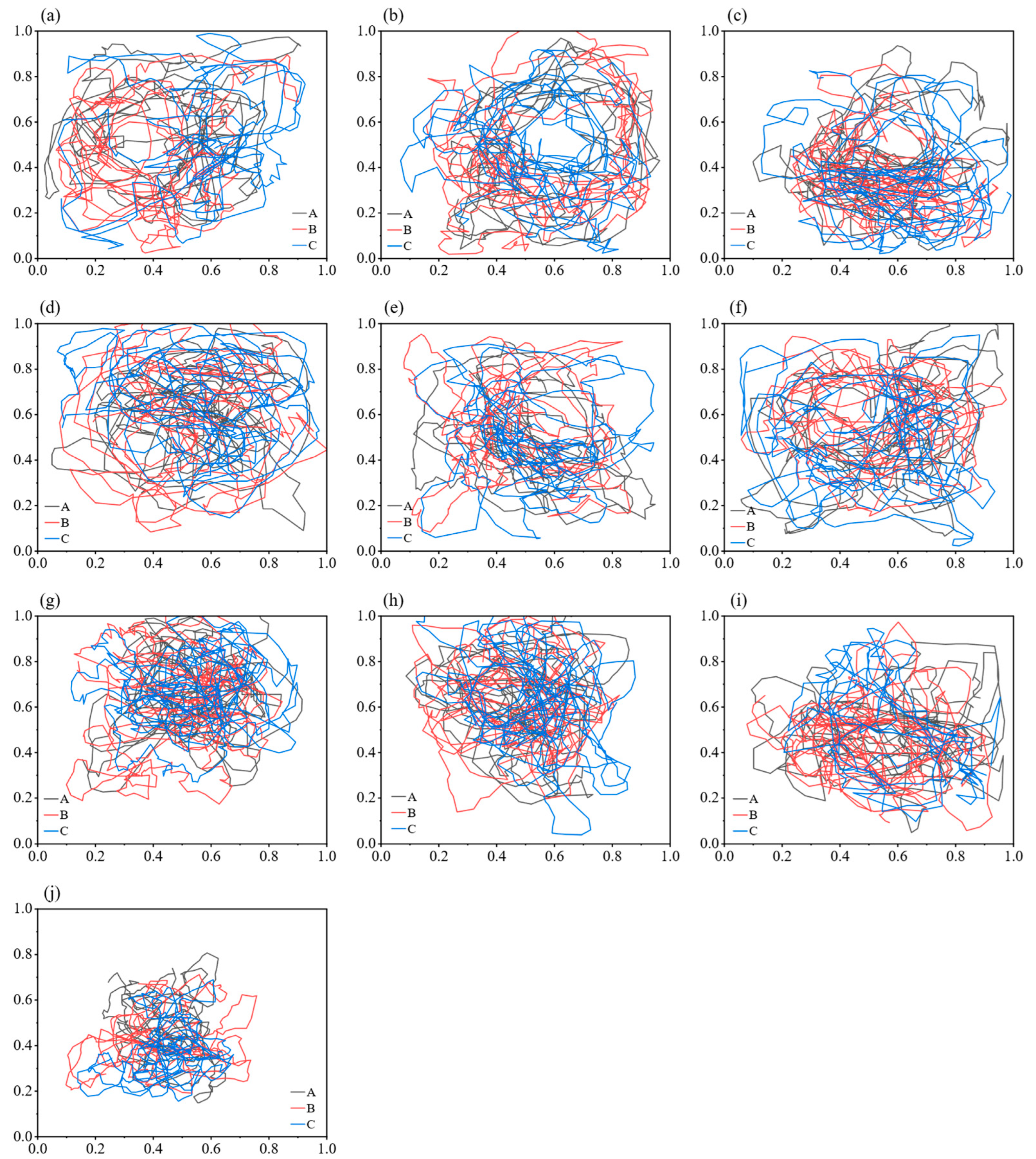
Swimming trajectories of experimental fish (D1). (a–i) represent L1–L9, and (j) represents L0. A, B, and C are the randomly selected trajectories of experimental fish from each treatment.
Figure 5.
Swimming trajectories of experimental fish (D1). (a–i) represent L1–L9, and (j) represents L0. A, B, and C are the randomly selected trajectories of experimental fish from each treatment.
Figure 6.
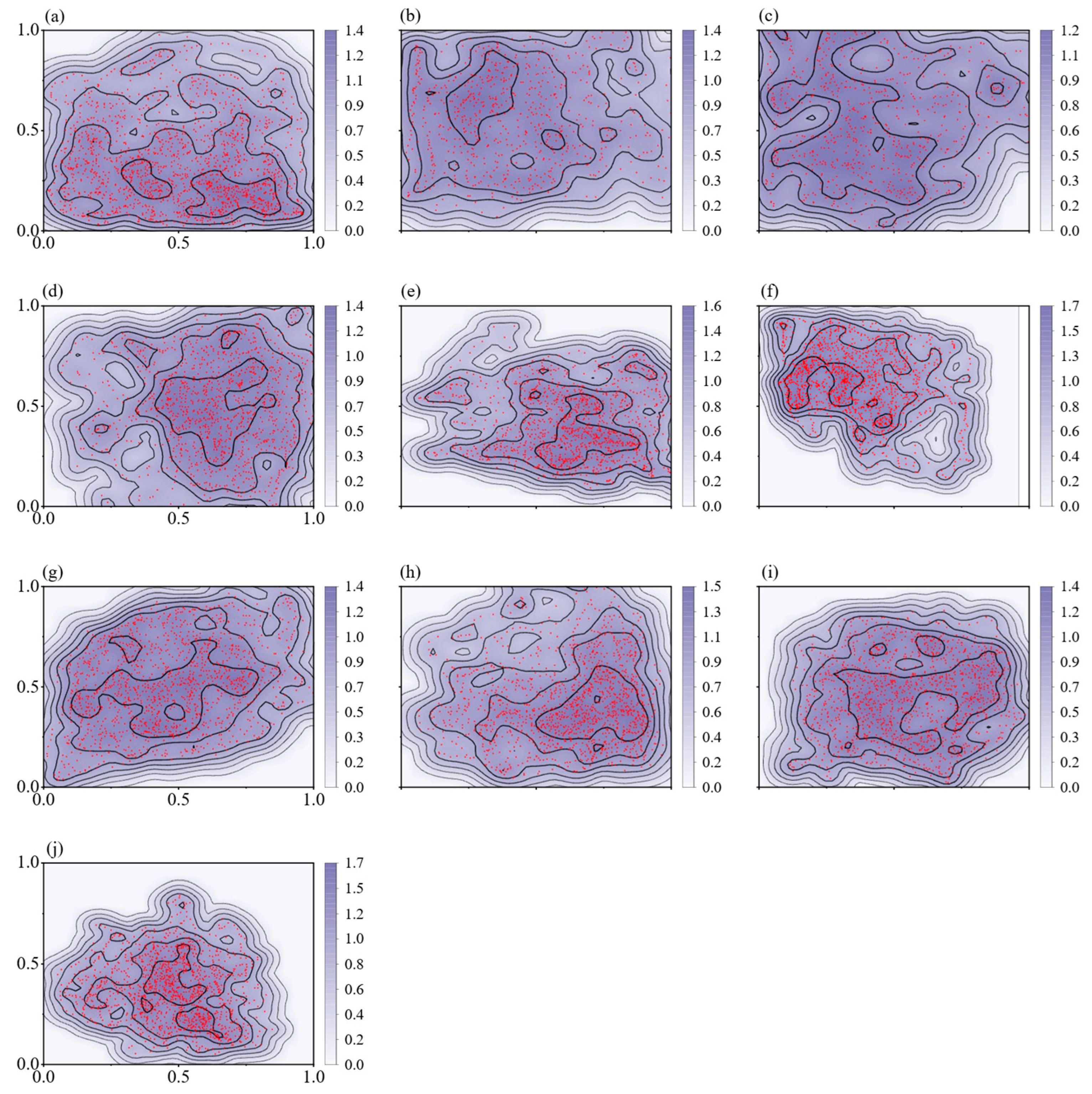
Distribution density map of the swimming trajectories of the experimental fish (D1). (a–i) represent L1–L9, and (j) represents L0.
Figure 6.
Distribution density map of the swimming trajectories of the experimental fish (D1). (a–i) represent L1–L9, and (j) represents L0.
Figure 7.
Swimming trajectories of experimental fish (D50). (a–i) represent L1–L9, and (j) represents L0. A, B, and C are the randomly selected trajectories of experimental fish from each treatment.
Figure 7.
Swimming trajectories of experimental fish (D50). (a–i) represent L1–L9, and (j) represents L0. A, B, and C are the randomly selected trajectories of experimental fish from each treatment.
Figure 8.
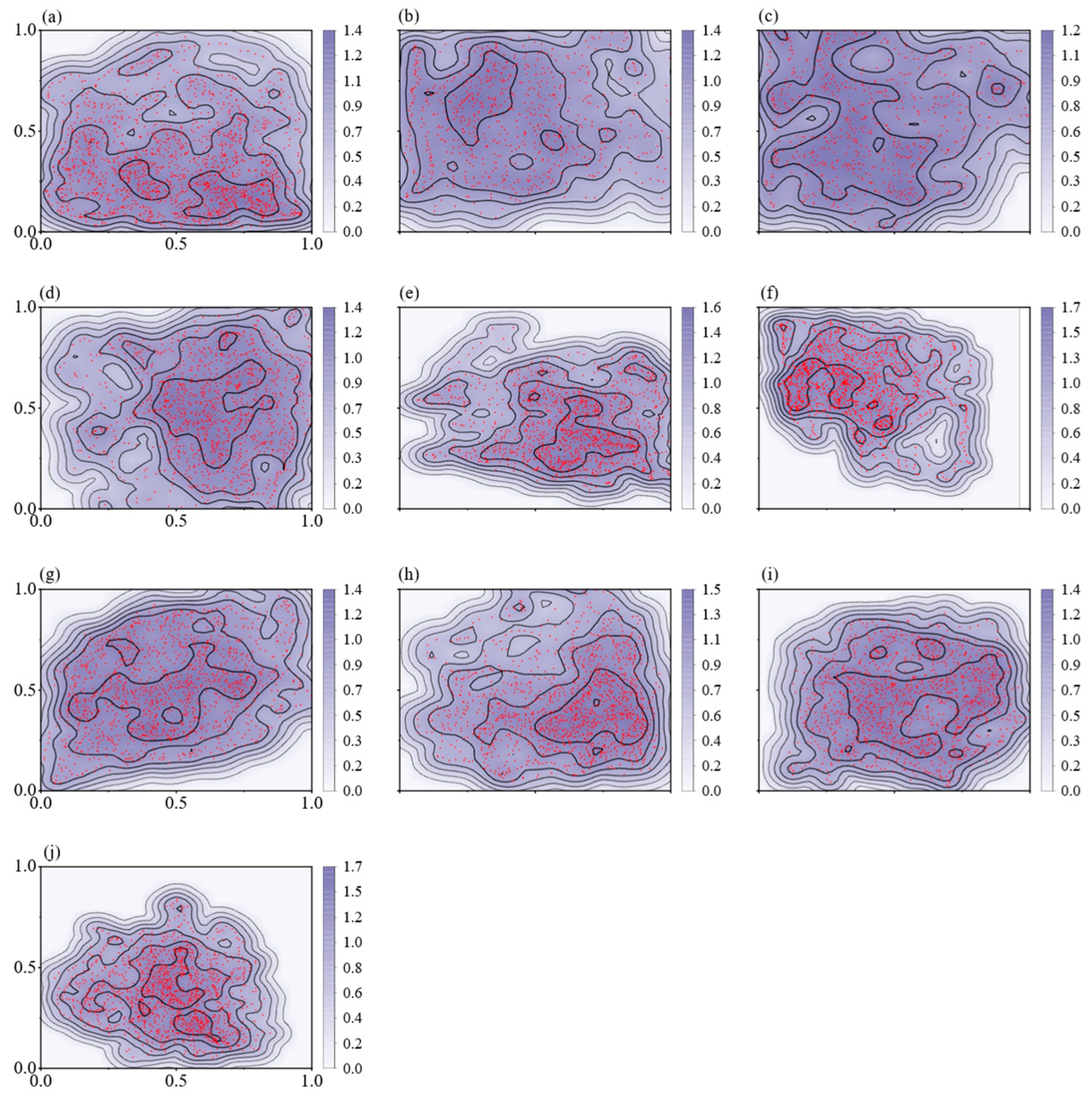
Distribution density map of the swimming trajectories of the experimental fish (D50). (a–i) represent L1–L9, and (j) represents L0.
Figure 8.
Distribution density map of the swimming trajectories of the experimental fish (D50). (a–i) represent L1–L9, and (j) represents L0.
Table 1.
Light condition treatments and the on/off schedule.
Table 1.
Light condition treatments and the on/off schedule.
| Light Treatment | Light Intensity | Photoperiod | Light ON/OFF Timing |
|---|
| L0 | 0 lx | 0L:24D | Constant darkness |
| L1 | 10 lx | 8L:16D | 08:00 ON/16:00 OFF |
| L2 | 10 lx | 16L:8D | 08:00 ON/00:00 OFF |
| L3 | 10 lx | 24L:0D | Constant illumination |
| L4 | 100 lx | 8L:16D | 08:00 ON/16:00 OFF |
| L5 | 100 lx | 16L:8D | 08:00 ON/00:00 OFF |
| L6 | 100 lx | 24L:0D | Constant illumination |
| L7 | 1000 lx | 8L:16D | 08:00 ON/16:00 OFF |
| L8 | 1000 lx | 16L:8D | 08:00 ON/00:00 OFF |
| L9 | 1000 lx | 24L:0D | Constant illumination |
Table 2.
The light intensity of illuminance measurement points.
Table 2.
The light intensity of illuminance measurement points.
| Red Point (2, 2) Illuminance (lx) | Blue Points (0, 0), (0, 4), (4, 4), (4, 0) Illuminance (lx) | Blue Points (1, 1), (1, 3), (3, 3), (3, 1) Illuminance (lx) |
|---|
| 10 | 2.48 | 5.03 |
| 100 | 45.52 | 55.03 |
| 1000 | 153.74 | 332.39 |
Table 3.
The definition of swimming behavior parameters.
Table 3.
The definition of swimming behavior parameters.
| Parameter | Definition |
|---|
| Average Swimming Speed (AS) | The distance moved per unit time, calculated as AS (m/s) = X/t, where X is the total movement distance (m) and t is the total movement time (s). |
| Average Angular Change (AC) | The angular deviation of the movement direction at time t2 relative to the direction at time t1, with the initial movement at time t0 serving as the reference. |
| Total Movement (TM) | The total distance moved by the experimental fish within time t, using the tip of the fish’s snout as the positional marker. |
| Average Distance from the Center (DC) | The average distance of the fish’s positional marker (tip of the snout) from the coordinate origin over the time period t. |
| Fastest Movement (FM) | The maximum distance covered by the experimental fish within a 1 s interval that exceeds twice its average swimming speed. |
Table 4.
Effects of light intensity and photoperiod on AS (D1), AC (D1), AC (D50), TM (D1), DC (D1), DC (D50), and FM (D1) by two-way ANOVA.
Table 4.
Effects of light intensity and photoperiod on AS (D1), AC (D1), AC (D50), TM (D1), DC (D1), DC (D50), and FM (D1) by two-way ANOVA.
| Parameter | Variation Sources | SS | df | F | p |
|---|
| AS (D1) | Light intensity | 0.060 | 2 | 8.20 | 0.002 |
| Photoperiod | 0.144 | 3 | 13.04 | <0.001 |
| Light intensity × Photoperiod | 0.115 | 6 | 5.23 | 0.001 |
| Residual | 0.088 | 24 | | |
| AC (D1) | Light intensity | 0.017 | 2 | 5.57 | 0.010 |
| Photoperiod | 0.039 | 3 | 8.23 | 0.001 |
| Light intensity × Photoperiod | 0.134 | 6 | 14.32 | <0.001 |
| Residual | 0.037 | 24 | | |
| AC (D50) | Light intensity | 246.405 | 2 | 13.80 | <0.001 |
| Photoperiod | 342.275 | 3 | 12.78 | <0.001 |
| Light intensity × Photoperiod | 184.209 | 6 | 3.44 | 0.014 |
| Residual | 214.226 | 24 | | |
| TM (D1) | Light intensity | 120.392 | 2 | 15.74 | <0.001 |
| Photoperiod | 155.127 | 3 | 13.52 | <0.001 |
| Light intensity × Photoperiod | 113.228 | 6 | 4.93 | 0.002 |
| Residual | 91.795 | 24 | | |
| DC (D1) | Light intensity | 0.000 | 2 | 0.01 | 0.986 |
| Photoperiod | 0.216 | 3 | 19.14 | <0.001 |
| Light intensity × Photoperiod | 0.114 | 6 | 5.07 | 0.002 |
| Residual | 0.090 | 24 | | |
| DC (D50) | Light intensity | 0.028 | 2 | 9.73 | 0.001 |
| Photoperiod | 0.163 | 3 | 38.44 | <0.001 |
| Light intensity × Photoperiod | 0.031 | 6 | 3.61 | 0.011 |
| Residual | 0.034 | 24 | | |
| FM (D1) | Light intensity | 0.368 | 2 | 8.72 | 0.001 |
| Photoperiod | 1.250 | 3 | 19.71 | <0.001 |
| Light intensity × Photoperiod | 0.881 | 6 | 6.95 | <0.001 |
| Residual | 0.507 | 24 | | |
Table 5.
Effects of light intensity and photoperiod on AS (D50), TM (D50), and FM (D50) by Kruskal–Wallis test.
Table 5.
Effects of light intensity and photoperiod on AS (D50), TM (D50), and FM (D50) by Kruskal–Wallis test.
| Parameter | Variation Sources | df | H | p |
|---|
| AS (D50) | Light intensity | 2 | 1.36 | 0.507 |
| Photoperiod | 3 | 22.55 | <0.001 |
| TM (D50) | Light intensity | 2 | 2.42 | 0.298 |
| Photoperiod | 3 | 20.70 | <0.001 |
| FM (D50) | Light intensity | 2 | 1.05 | 0.593 |
| Photoperiod | 3 | 21.03 | <0.001 |
Table 6.
Effects of light treatment groups and treatment duration on the AS, AC, TM, DC, and FM of rainbow trout.
Table 6.
Effects of light treatment groups and treatment duration on the AS, AC, TM, DC, and FM of rainbow trout.
| Parameter | Group | D1 | D50 |
|---|
| AS | L0 | 0.42 ± 0.04 Abcd | 0.33 ± 0.01 Bb |
| L1 | 0.58 ± 0.08 Bab | 0.65 ± 0.01 Aa |
| L2 | 0.42 ± 0.06 Bbcd | 0.65 ± 0.03 Aa |
| L3 | 0.61 ± 0.04 Ba | 0.68 ± 0.03 Aa |
| L4 | 0.58 ± 0.09 Bab | 0.68 ± 0.03 Aa |
| L5 | 0.31 ± 0.12 Bd | 0.52 ± 0.03 Aa |
| L6 | 0.35 ± 0.02 Bcd | 0.68 ± 0.03 Aa |
| L7 | 0.50 ± 0.04 Babc | 0.60 ± 0.11 Aa |
| L8 | 0.47 ± 0.01 Babcd | 0.68 ± 0.03 Aa |
| L9 | 0.57 ± 0.04 Bab | 0.70 ± 0.02 Aa |
| AC | L0 | 38.41 ± 1.56 Bc | 44.35 ± 3.18 Aabc |
| L1 | 35.21 ± 4.44 Bc | 39.86 ± 1.37 Aabc |
| L2 | 54.57 ± 9.88 Aab | 33.85 ± 4.11 Bcd |
| L3 | 41.79 ± 4.56 Bbc | 48.97 ± 1.93 Ad |
| L4 | 37.48 ± 1.20 Bc | 48.97 ± 1.93 Aab |
| L5 | 48.11 ± 4.39 Aabc | 45.35 ± 3.37 Babc |
| L6 | 59.87 ± 5.96 Aa | 45.21 ± 2.86 Babc |
| L7 | 48.55 ± 2.28 Babc | 51.44 ± 0.44 Aa |
| L8 | 34.89 ± 2.95 Bc | 51.09 ± 2.91 Aa |
| L9 | 38.94 ± 0.76 Bc | 41.86 ± 0.12 Abcd |
| TM | L0 | 12.64 ± 1.39 Acde | 9.98 ± 0.12 Bb |
| L1 | 21.36 ± 0.12 Ba | 16.80 ± 0.15 Ab |
| L2 | 12.77 ± 1.58 Bcde | 18.76 ± 0.94 Aab |
| L3 | 18.56 ± 1.14 Aab | 19.42 ± 0.82 Aab |
| L4 | 15.48 ± 2.23 Bbcd | 20.83 ± 0.82 Aa |
| L5 | 9.43 ± 3.89 Be | 15.94 ± 0.84 Ab |
| L6 | 10.35 ± 0.43 Bde | 20.50 ± 0.79 Aab |
| L7 | 15.35 ± 1.22 Bbcd | 20.22 ± 1.70 Aab |
| L8 | 14.90 ± 1.07 Bbcde | 20.87 ± 0.67 Aa |
| L9 | 17.29 ± 1.13 Aabc | 18.76 ± 5.08 Ab |
| DC | L0 | 0.57 ± 0.08 Ac | 0.62 ± 0.03 Ad |
| L1 | 0.65 ± 0.02 Bbc | 0.75 ± 0.00 Abcd |
| L2 | 0.73 ± 0.04 Bab | 0.75 ± 0.04 Aabc |
| L3 | 0.86 ± 0.07 Aa | 0.70 ± 0.17 Bcd |
| L4 | 0.84 ± 0.04 Aa | 0.85 ± 0.04 Aa |
| L5 | 0.66 ± 0.01 Bbc | 0.73 ± 0.01 Abcd |
| L6 | 0.73 ± 0.04 Bab | 0.78 ± 0.05 Aabc |
| L7 | 0.72 ± 0.04 Babc | 0.84 ± 0.03 Aa |
| L8 | 0.79 ± 0.01 Bab | 0.82 ± 0.03 Aab |
| L9 | 0.74 ± 0.06 Bab | 0.77 ± 0.04 Aabc |
| FM | L0 | 1.08 ± 0.07 Acde | 0.81 ± 0.02 Bc |
| L1 | 1.58 ± 0.22 Aab | 1.47 ± 0.06 Bab |
| L2 | 1.05 ± 0.12 Bcde | 1.55 ± 0.14 Aab |
| L3 | 1.70 ± 0.01 Aa | 1.64 ± 0.08 Aab |
| L4 | 1.56 ± 0.15 Aab | 1.64 ± 0.08 Aa |
| L5 | 0.82 ± 0.34 Be | 1.23 ± 0.09 Ab |
| L6 | 0.95 ± 0.08 Bde | 1.61 ± 0.10 Aa |
| L7 | 1.27 ± 0.08 Babcd | 1.47 ± 0.24 Aab |
| L8 | 1.19 ± 0.04 Bbcde | 1.65 ± 0.13 Aa |
| L9 | 1.41 ± 0.02 Babc | 1.56 ± 0.07 Aa |
Table 7.
Correlations between feeding behaviors of rainbow trout (D1).
Table 7.
Correlations between feeding behaviors of rainbow trout (D1).
| Parameter | AS | AC | TM | DC | FM |
|---|
| AS | -- | −0.47 ** | 0.85 ** | 0.41 ** | 0.89 ** |
| AC | | -- | −0.50 ** | −0.11 | −0.51 ** |
| TM | | | -- | 0.28 | 0.79 ** |
| DC | | | | -- | 0.40 * |
| FM | | | | | -- |
Table 8.
Correlations between feeding behaviors of rainbow trout (D50).
Table 8.
Correlations between feeding behaviors of rainbow trout (D50).
| Parameter | AS | AC | TM | DC | FM |
|---|
| AS | -- | 0.04 | 0.81 ** | 0.54 ** | 0.82 ** |
| AC | | -- | 0.27 | 0.60 ** | 0.11 |
| TM | | | -- | 0.63 ** | 0.81 ** |
| DC | | | | -- | 0.52 ** |
| FM | | | | | -- |