Visual Characterization of Male and Female Greenshell™ Mussels (Perna canaliculus) from New Zealand Using Image-Based Shape and Color Analysis

Abstract

Machine vision/image analysis is used in the sorting and handling of many aquatic species. Pictures of 474 New Zealand Greenshell™ (Perna canaliculus, Gmelin, 1791) whole unopened mussels (215 females and 259 males) from the top and from the side were analyzed to evaluate if visual attributes (size, shape, and color) can be used to differentiate gender. Size (length, width, height, and view area), color, and shape (by elliptic Fourier analysis and by ray length-ray angle analysis) were analyzed and differences by gender tested. Application of Artificial Neural Networks (ANN), Principal Component Analysis (PCA), Canonical Discriminant Analysis (CDA), and Random Forest (RF) to the shape parameters failed to reliably predict gender. Comprehensive morphometric and color characterization of males and females, as well as shape parameters, are presented as a reference for future image-based research. The parasitic crustacean pea crab can change the shape of mussel shells, and elliptic Fourier analysis can quantify this difference.

1. Introduction

The New Zealand Greenshell™ mussel, Perna. canaliculus, is widely farmed in New Zealand, and is the most important commercial shellfish in both domestic and export markets [1].

Mussel meat appears and tastes differently depending on harvest location and time, maturity of the mussel, and genetic variation [2]. Mussels harvested at spawning season normally have a lower quality due to a reduction in lipids and carbohydrates for energy- and nutrient-rich gamete release, and low food availability in the environment [3]. Zhou et al. [4] found differences in both lipid classes and fatty acid profiles from male and female Greenshell™ mussels.

Automation is already part of mussel processing in New Zealand [5]. Prediction of the gender of unopened mussels by shape analysis or other visual attributes would offer a commercial advantage in separating mussels by gender. Zieritz and Aldridge [6] observed that three of five study populations of freshwater mussel Anodonta anatina displayed significant sexual shell width dimorphism: female shells were significantly wider than males. Additionally, in two of the populations, female shells were significantly thinner than those of the males. Kotrla and James [7] reported that the freshwater mussels Villosa villosa and Elliptio icterina exhibited sexual dimorphism. Variables describing the ventro-posterior region of the shell showed discrimination between sexes of both species. Trivellini et al. [8] showed non-sexual dimorphism in Mytilus edulis platensis, a marine mussel. Steffani and Branch [9] reported that Mytilus galloprovincialis shells were narrower at wave-exposed sites. Reimer and Tedengren [10] reported that blue mussels (Mytilus edulis) exposed to their predator starfish Asterias rubens were significantly smaller in shell length, height, and width but had a significantly larger posterior adductor muscle compared to the mussels without predator pressure. They concluded that predator-induced morphological plasticity existed in M. edulis. Telesca et al. [11] reported on blue mussel shell shape plasticity based on the natural environment.

Hickman [12] used total length to predict the weight of P. canaliculus. Allometry depended on environmental conditions: raft- and shore-grown mussels had morphologically distinct forms. Inter-tidally grown mussels were wider, less high, and heavier. Thejasvi et al. [13] developed length–weight relationships for P. viridis, as well as length–breadth and length–width equations. The latter equations were linear, while the length–weight equation was a power equation.

Machine vision/image analysis can be used to measure dimensions [14], and view the area [15], shape [16], and color [17] of foods in general, and seafood in particular. A commonly used tool to evaluate the shape of shells is elliptic Fourier analysis (EFA) [18]. Costa et al. [19] used EFA to analyze the shapes of Ruditapes decussatus and Ruditapes philippinarum from the Mediterranean and the Atlantic. They correctly discriminated between the two at 99% accuracy.

Palmer et al. [20] discriminated between geographical groups of the Mediterranean clam (Chamelea gallina) by shape analysis using EFA. They reported an error rate of less than 1%. Ruffino et al. [21] used linear (shell length, width, height, and total weight) and geometric morphometric (EFA and landmark-based) methods to distinguish venus clams from Portuguese coastal water. Geometric morphometric methods had 0–6% misclassification rates, while linear methods had about 17%. Costa et al. [22] correctly classified (96%) two clams (Tapes decussatus and Tapes philippinarum) by a combination of EFA and partial least squares discriminant analysis. Marquez and Van der Molen [23] quantified the shell shape variation of razor clams along 3700 km of longitudinal range of the Atlantic coast of South America using EFA. They reported that shell slenderness and curvature were associated mainly with salinity and the water depth of the localities. There were significant shell shape variations along the longitudinal range. Preston et al. [24] reported that the freshwater pearl mussel found in many rivers in Ireland and UK had a plastic phonotype, with a shape change with water pH.

It is evident that both dimensions and shape description tools are important in quantitatively determining the visual characteristics of mussels. The objective of this study was to measure several visual attributes of P. canaliculus by image analysis for both genders.

2. Materials and Methods

2.1. Greenshell™ Mussel Samples

Live New Zealand Greenshell™ mussels (Perna canaliculus, Gmelin, 1791) were harvested from Haro Partnership Mussel Farm located in Marlborough Sound, New Zealand on 5 November 2013. The exact environmental conditions (substrate type, water flow, etc.) that the mussels were cultured in were not known. All mussels were rehydrated immediately in seawater tanks at a temperature of 12 °C and salinity of 3.3% overnight at the facilities of Plant and Food in Mt. Albert, Auckland before being processed to allow intra-valvular fluids to be replenished. As shown in Figure 1, the mussels were placed in a light box, 5 mussels at a time. Small pieces of white “silly putty” were placed in 5 locations, and the mussels were placed on them to stabilize the mussels for both top view and side view images. The picture on the left in Figure 1 shows the silly putty under the mussels that keeps them upright. Whole mussels were weighed individually, and the meat was also weighed after shucking.

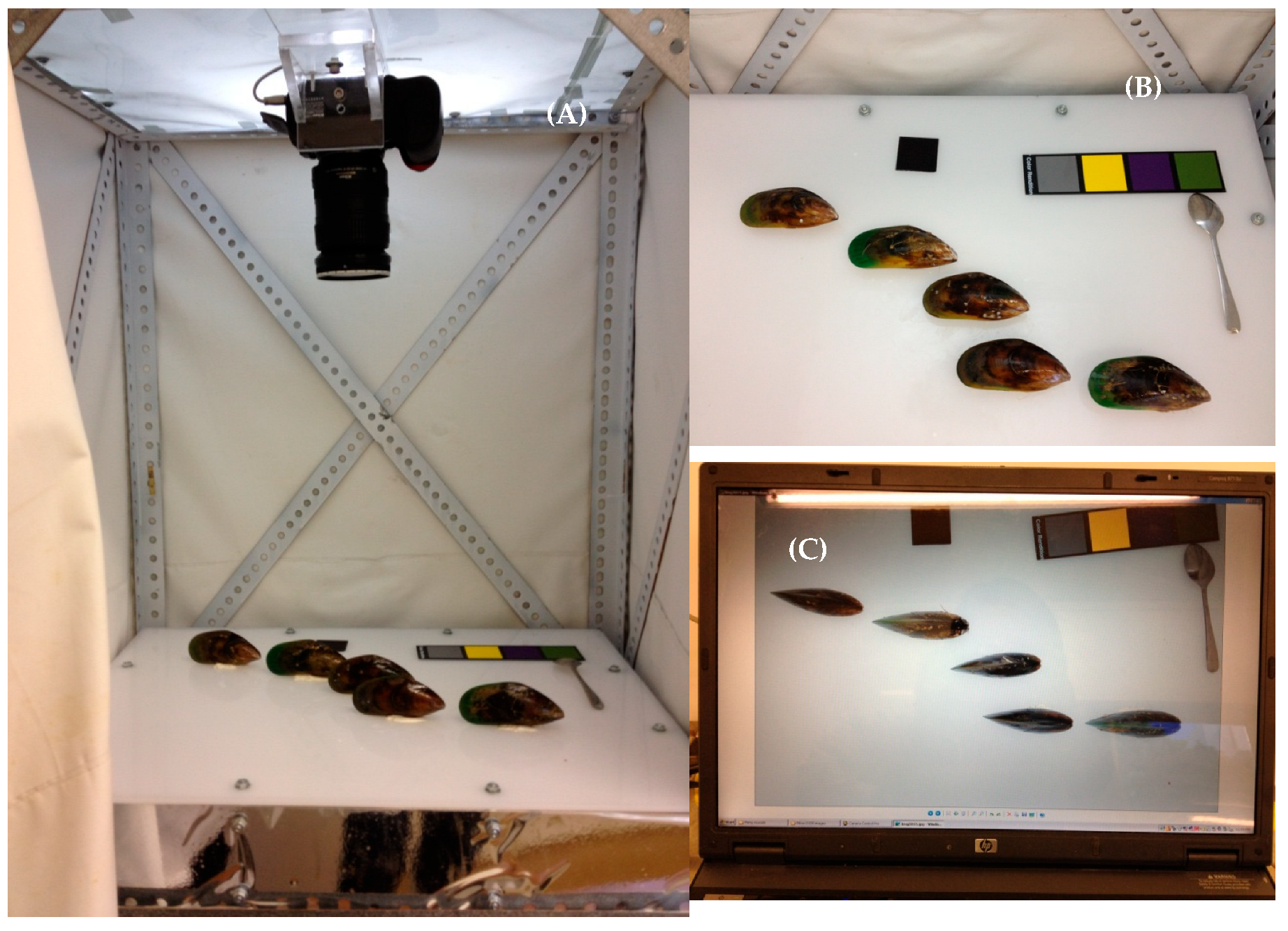
2.2. Acquiring Whole Mussel Images

A light box was used (Figure 1) for constant illumination. As described in detail by Luzuriaga et al. [25], there were 2 sets of fluorescent lights (top and bottom), separated from the experimental space by a 51% transmissive diffuser. The inside surface of the top light was covered with a polarizing sheet (Rosco Stamford, CT, USA).

Figure 1. Experimental setup to take pictures. (A): Light box and camera. (B): Five un-shucked mussels, top view; colour and size reference (C): Five un-shucked mussels, side view [1].

Figure 1. Experimental setup to take pictures. (A): Light box and camera. (B): Five un-shucked mussels, top view; colour and size reference (C): Five un-shucked mussels, side view [1].

A Nikon D300S digital camera (Nikon Corp., Tokyo, Japan), an 18–200 mm Nikkor zoom lens, and a circular polarizing filter were used to take pictures. The settings of the camera are given in

Table 1. Nikon D300 camera control settings for front-lighted images.

Camera Settings	Value
Exposure Mode	Manual
Shutter Speed	1.6 s
Aperture	f/6.3
Exposure Compensation	0 EV
ISO sensitivity	200
White Balance	Preset manual
Image size (pixels)	2144 × 1424

. A Nikon Camera Control Pro 2 (Nikon Corp, Tokyo, Japan) was used to control the camera, take pictures, and transfer the image files to a laptop computer. Each image contained a 4 × 4 cm black metallic square as a size reference. Therefore, measurements such as length, width, height, view area, etc., were converted to real units (cm, cm²). Also, a color reference (Gretag Color Checker, X-Rite Inc., Grand Rapids, MI, USA), previously measured by a hand-held Minolta color meter, was in every picture to help with calibrating color during image analysis.

2.3. Determination of Gender

Whole mussels were manually shucked using a blunt shucking knife. The gender was determined by meat color (cream to light-colored flesh representing males and an orange to apricot color for females). This visual method is used widely in the industry, and the potential for misidentification may occur when the gonad tissue is not clearly visible. Our determination was not based on histological inspection. This is a limitation in our study. Of the 474 mussels, 4 contained pea crabs (Nepinnotheres novaezelandiae), a crustacean parasite of the green-lipped mussel.

2.4. Color Analysis

Images obtained were analyzed by the software LensEye-NET version 2.1 (ECS, Gainesville, FL, USA). Each image was segmented to recognize the mussels. The color of the whole image was calibrated by using the color reference. The number of pixels of the size reference were counted, and the pixel dimensions were converted to real-world cm/cm² dimensions.

The average L*, a*, and b* of every pixel in the view area of a mussel were calculated. In addition, the pixels with a* value < −5 were classified as “green” pixels, and their percentage in the total view area was calculated.

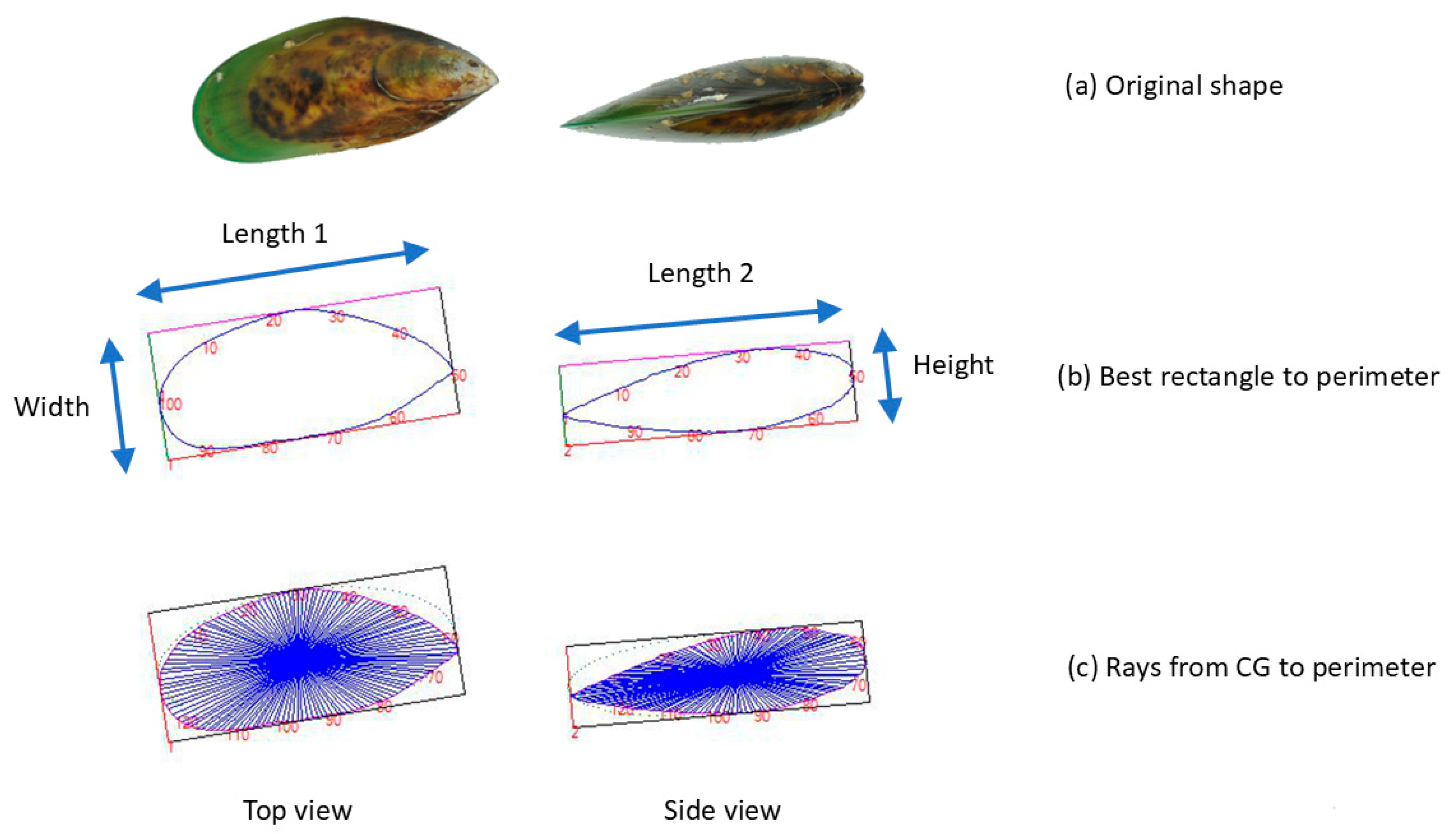
2.5. Image Analysis: Determination of Dimensions and Shape

Each mussel was fitted with the “best” rectangle around it, using LensEye-NET software. This is the rectangle that touches the mussel perimeter externally, and has the minimum area of all tested rectangle angles. Figure 2a presents the measurements of length, width, and height of the mussels. Since two length measurements could be made (from the top view and from the side view), their average was taken to be used as the length.

For normalized ray length—ray angle analysis, 128 points were defined that lay along equal angle divisions around the perimeter. Then, the best rectangle and perimeter points were rotated to make the rectangle horizontal. Distances from the perimeter points to the center of gravity of the polygon were taken as rays. The ray lengths were normalized by dividing the individual ray lengths by that of the longest ray, therefore, making ray lengths comparable between mussels of different sizes and orientations. Leyva-Valencia et al. [26] call this the “fan based” approach.

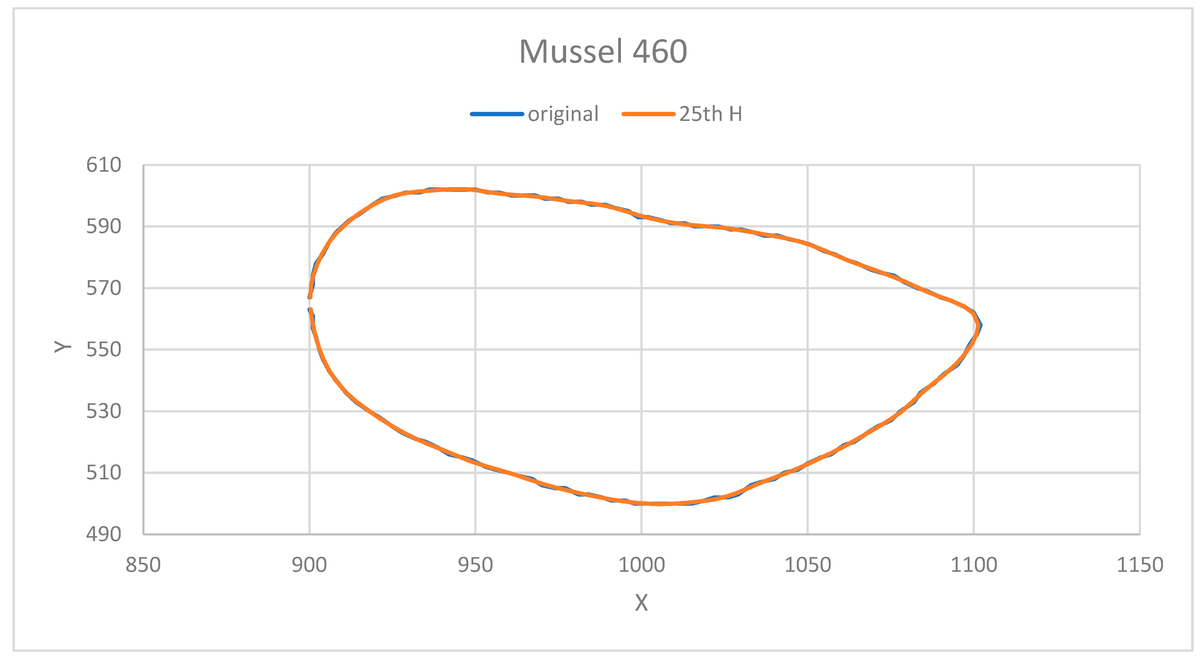
2.6. Elliptic Fourier Analysis

The software LensEye-NET was used. The method described by Ninomiya [27] was adopted. Briefly, in this method, the perimeter is divided into equally spaced points (128 in this study). Parameters A, B, C, and D are calculated based on these points using elliptic Fourier equations. These parameters can be used to calculate X and Y data for each perimeter point, depending on the number of harmonics included in the calculation: the more harmonics, the closer the predicted shape to the original shape. Then, the A, B, C, and D parameters are normalized for orientation, size, and starting point to obtain normalized parameters a, b, c, and d. These can be used to calculate normalized X Y points of the perimeter depending on the number of harmonics included. As an error tolerance limit regarding the number of harmonics to select, the recommendation of MacLeod [28] was used. First, the perimeter of the polygon composed of the 128 original X Y points was calculated. Then, for each added harmonic, the perimeter of the polygon composed of the calculated X Y points was obtained. When the difference was less than 1% based on the original perimeter, then this harmonic was selected as the critical harmonic.

The normalized parameters were used for statistical analysis. Normalization removed the effect of size, orientation, and starting point for the analysis.

2.7. Neural Networks Analysis

Statistica 7.1 (StatSoft Inc., Tulsa, OK, USA) was used to attempt to distinguish gender by mussel shape. For this, up to and including the 25th harmonic was taken, and the normalized EPA parameters were fed to several neural network configurations. One and two hidden layers and different numbers of nodes in the hidden layers were tried.

2.8. Principal Component Analysis

This method aims to reduce the number of original independent variables (shape parameters a, b, c, and d) with minimum information loss. The number of principal components to explain 90% of variation in the shape parameters data was calculated. Then several principal components were examined to correctly predict gender. Statistica 7.1 was used.

2.9. Canonical Discriminant Analysis

In this method, linear combinations of original shape parameters were chosen to have the highest ratio of between-group to within-group variance, orthogonal to any previously calculated discriminant dimensions. GenStat 20 (Hempstead, UK) was used for analysis.

2.10. Random Forests Analysis

The Random Forests procedure takes subsets of the data (both variables and observations) and builds a decision tree model for each. Each model can be used to predict gender for the observations that were not used to build it, similar to a cross-validated misclassification rate. For each variable, the procedure compares the accuracy (proportion of the observations that were used to fit the model that are correctly classified) of models including and excluding that variable; potentially useful classifying variables are ones where the accuracy is worse when they are not included in the model. GenStat 20 (Hempstead, UK) was used for analysis.

3. Results and Discussion

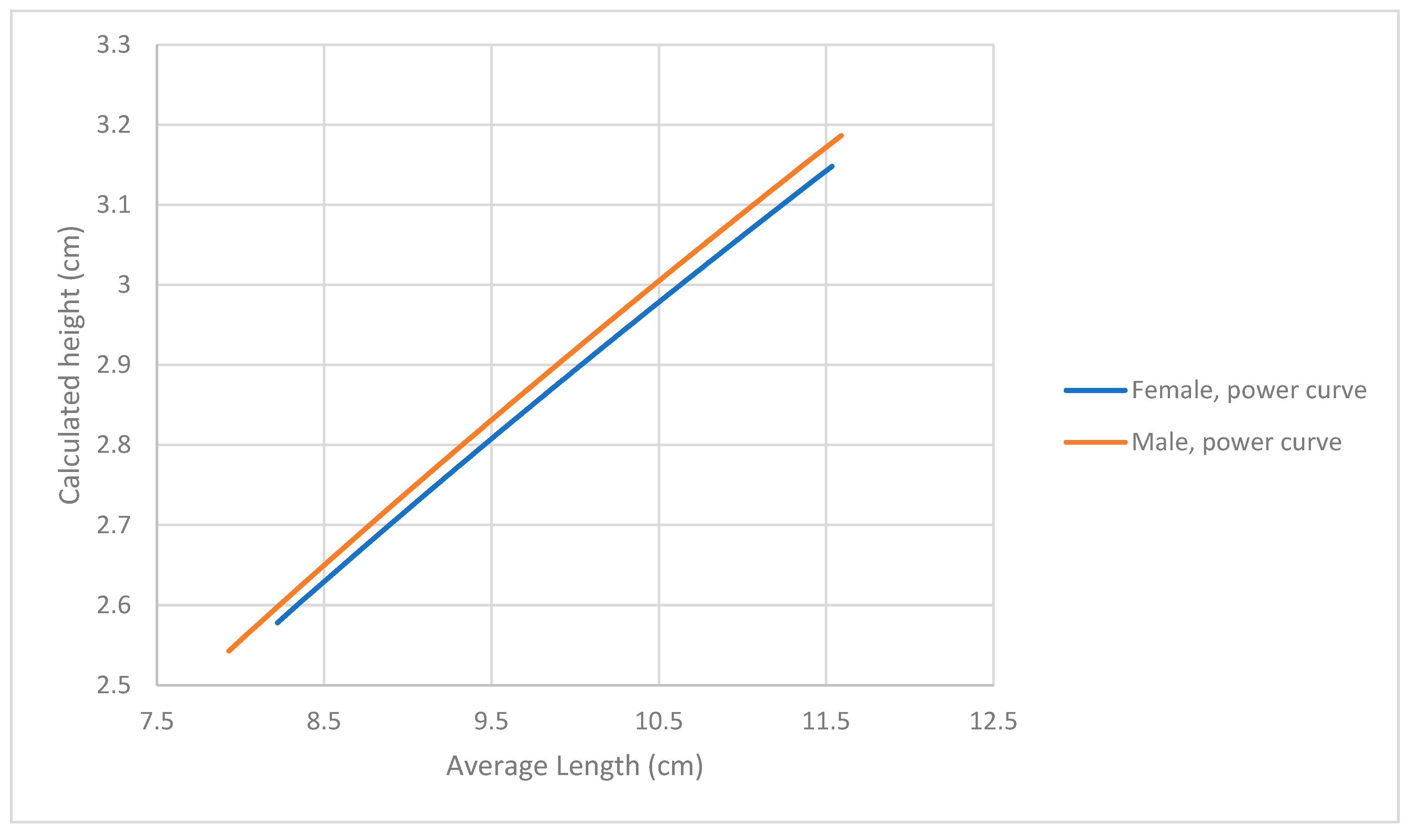
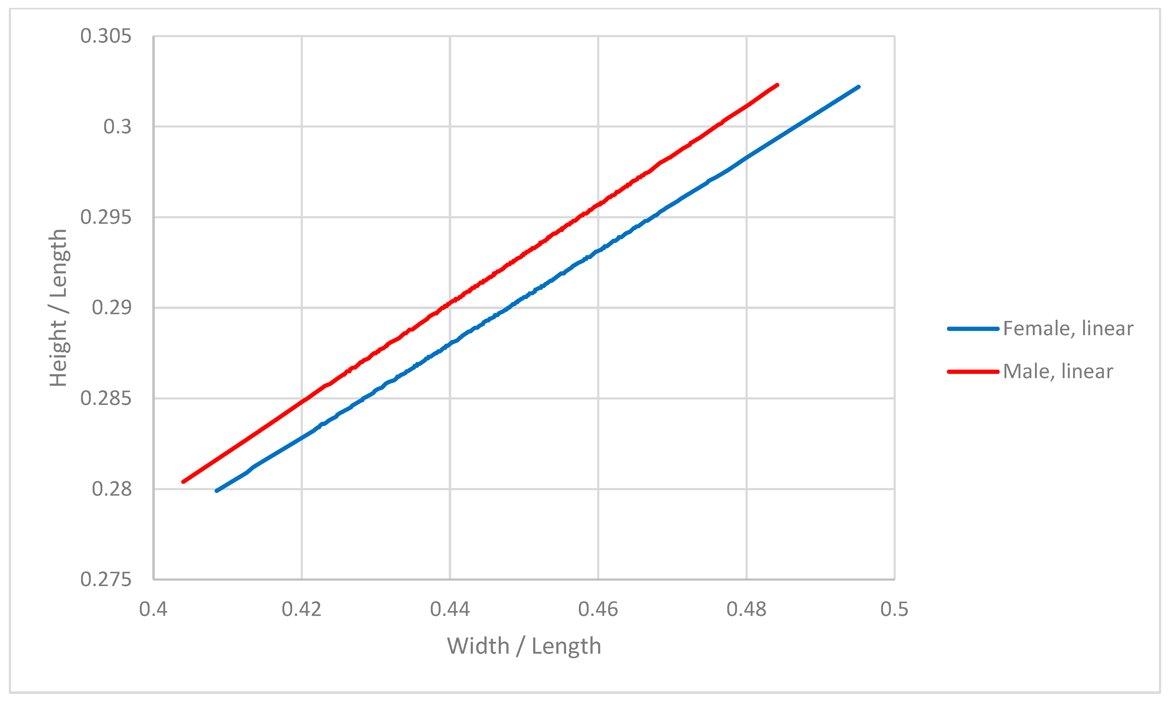
3.1. Analysis of Dimensions

Table 2. Average dimensional data on all of the mussels, female mussels only, and male mussels only.

	Average Length (cm)			Width (cm)			Height (cm)
	Overall	Female	Male	Overall	Female	Male	Overall	Female	Male
Average	10.01	10.03	10.00	4.47	4.47	4.48	2.91	2.90	2.92
St Dev	0.63	0.61	0.66	0.26	0.25	0.27	0.15	0.15	0.15
Min	7.93	8.22	7.93	3.69	3.69	3.69	2.35	2.43	2.35
Max	11.59	11.55	11.59	5.11	5.11	5.07	3.3	3.22	3.3

St Dev: standard deviation of the averages presented.

presents the dimensional data of all mussels (overall, n = 474), female mussels (n = 215), and male mussels (n = 259). It can be seen that the average values of length, width, and height of female and male mussels are within each other’s standard deviation. The results of t statistics with unequal variances confirm this conclusion: for length t stat = −0.814, p two tail = 0.416; for width, t stat = −0.254, p two tail = 0.799; and for height t stat = −1.449, p two tail = 0.148. Therefore, separation of gender by using the average dimensional parameters of length, width, and thickness alone is not possible.

In addition, combined dimensions of width/length and height/length were evaluated. The plot of the latter for female and male mussels is given in Figure 3, top. Although statistically not significant, this finding suggests that there may be a trend in the height of female mussels being less than that of a male of the same length (

Table 3. Parameters of equation fits to height vs. length and to weight vs. area data for female and male mussels.

	Height vs. Length		Weight vs. Area
	Female	Male	Female	Male
Y = A + B X
A	1.195 ± 0.247	1.186 ± 0.187	0.793 ± 5.654	−5.269 ± 4.541
B	0.170 ± 0.025	0.173 ± 0.019	1.705 ± 0.162	1.881 ± 0.13
R2	0.463	0.564	0.666	0.757
Y = A XB
A	0.745 ± 1.214	0.742 ± 1.155	1.722 ± 1.393	1.105 ± 1.306
B	0.589 ± 0.084	0.595 ± 0.063	1.000 ± 0.094	1.125 ± 0.075
R2	0.469	0.575	0.673	0.769
Y = Co + C1X + C2X2
C0	−0.334	−0.426	−4.189	−21.362
C1	0.479	0.503	1.999	2.846
C2	−0.016	−0.017	−0.004	−0.014
R2	0.466	0.569	0.667	0.759

). Even more interesting was the plot of height/length vs. width/length for mussels of different gender (Figure 3, bottom). There seems to be a trend of female height/length being less than that of a male of the same width/length value. The parameters of the linear fit to the above relationship were for female mussels A = 0.175 ± 0.05 and for males A = 0.17 ± 0.048. The 95% confidence intervals overlap; therefore, they cannot be statistically distinguished. The 95% confidence intervals for the B values of females and males also overlap. However, the combination of dimensions with other data should be tried if gender can be separated in a statistically significant manner.

The average view areas of mussels are given in

Table 4. View area, percent green, and critical EFA harmonic of all of the mussels, female mussels, and male mussels.

	View Area (Square cm)			Percent Green: a* < −5			Critical EFA Harmonic
	Overall	Female	Male	Overall	Female	Male	Overall	Female	Male
Average	34.68	34.70	34.66	20.36	20.91	19.91	9.77	9.74	9.79
St Dev	3.93	3.77	4.07	8.30	8.12	8.43	1.36	1.27	1.43
Min	23.05	24.29	23.05	0	1.44	0	6	6	7
Max	43.34	43.09	43.34	52.44	40.36	52.44	17	14	17

St Dev: standard deviation of the averages presented.

. It is evident that there is a wide range seen from the min and max values. Also, there is no statistical difference between female and male average view area values, judged by the overlapping standard deviation ranges.

3.2. Analysis of Weight vs. Area

The parameters of the various equations to predict weight in terms of view area are given in Table 3. It can be observed that the R² values are lower than those of many other species, e.g., fish where R² values can reach a high 0.9 range [29]. It can also be observed that statistically there is no difference between the parameters of female and male mussels. Therefore, this relationship alone cannot discriminate between genders.

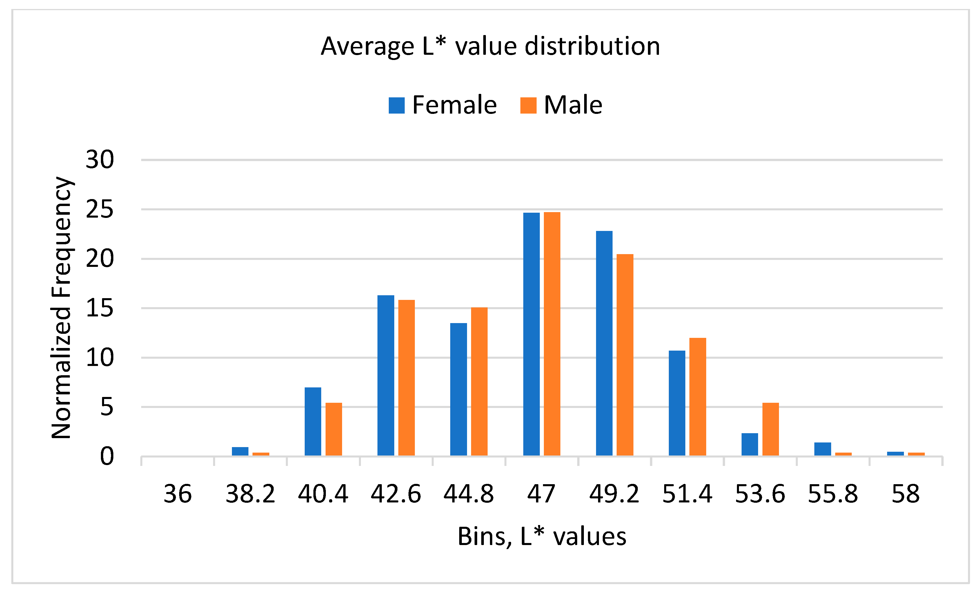
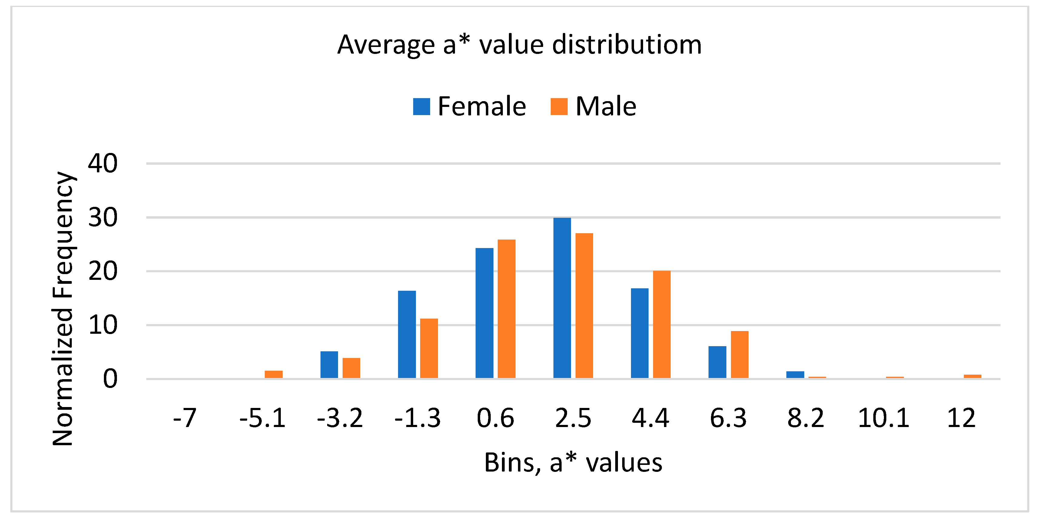
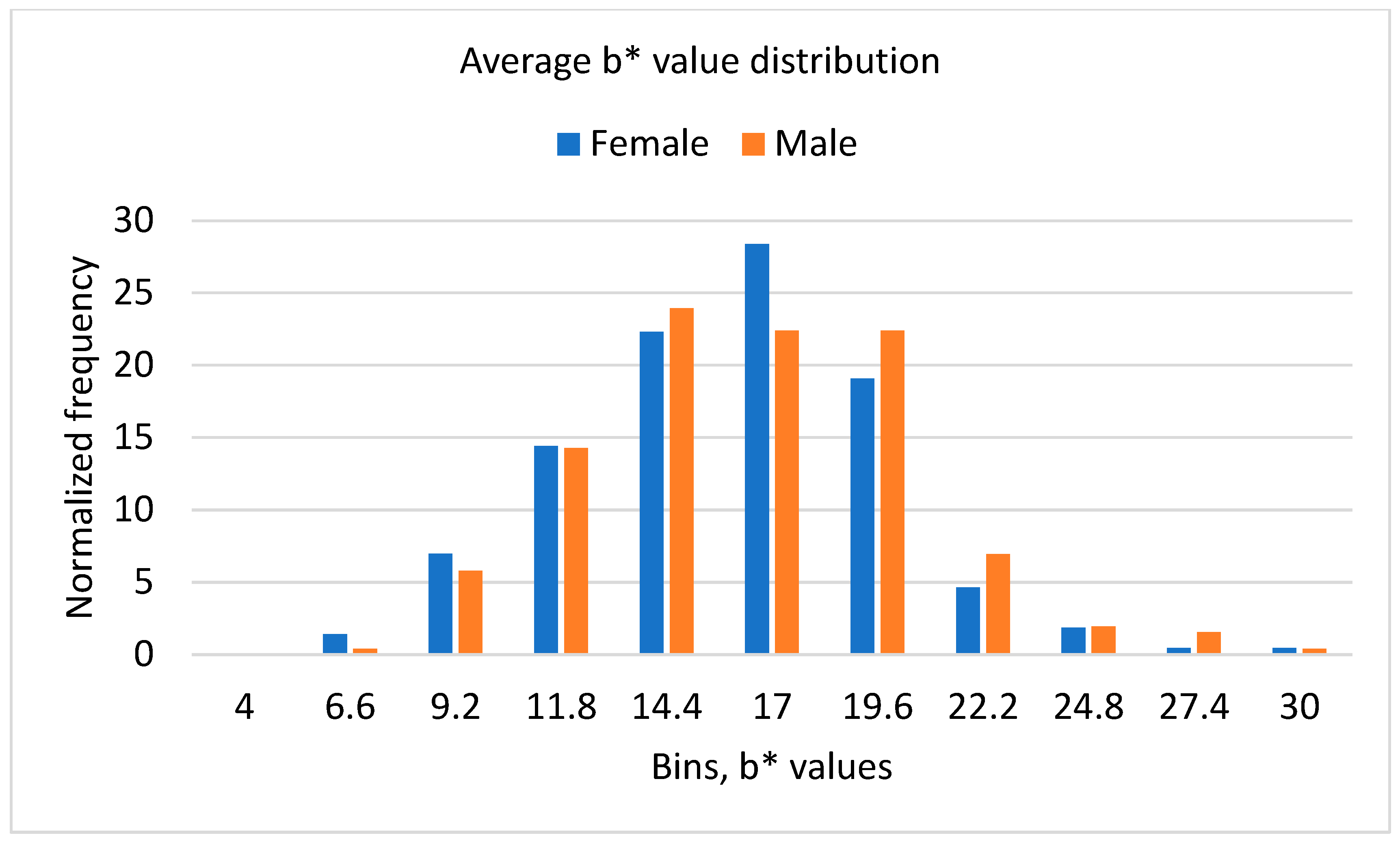
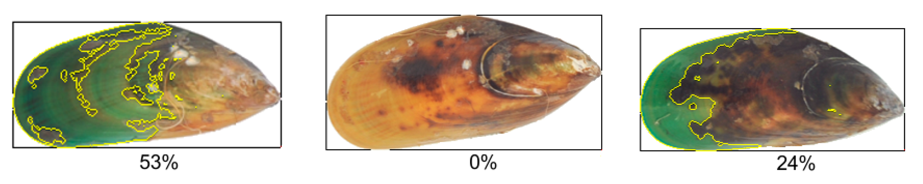
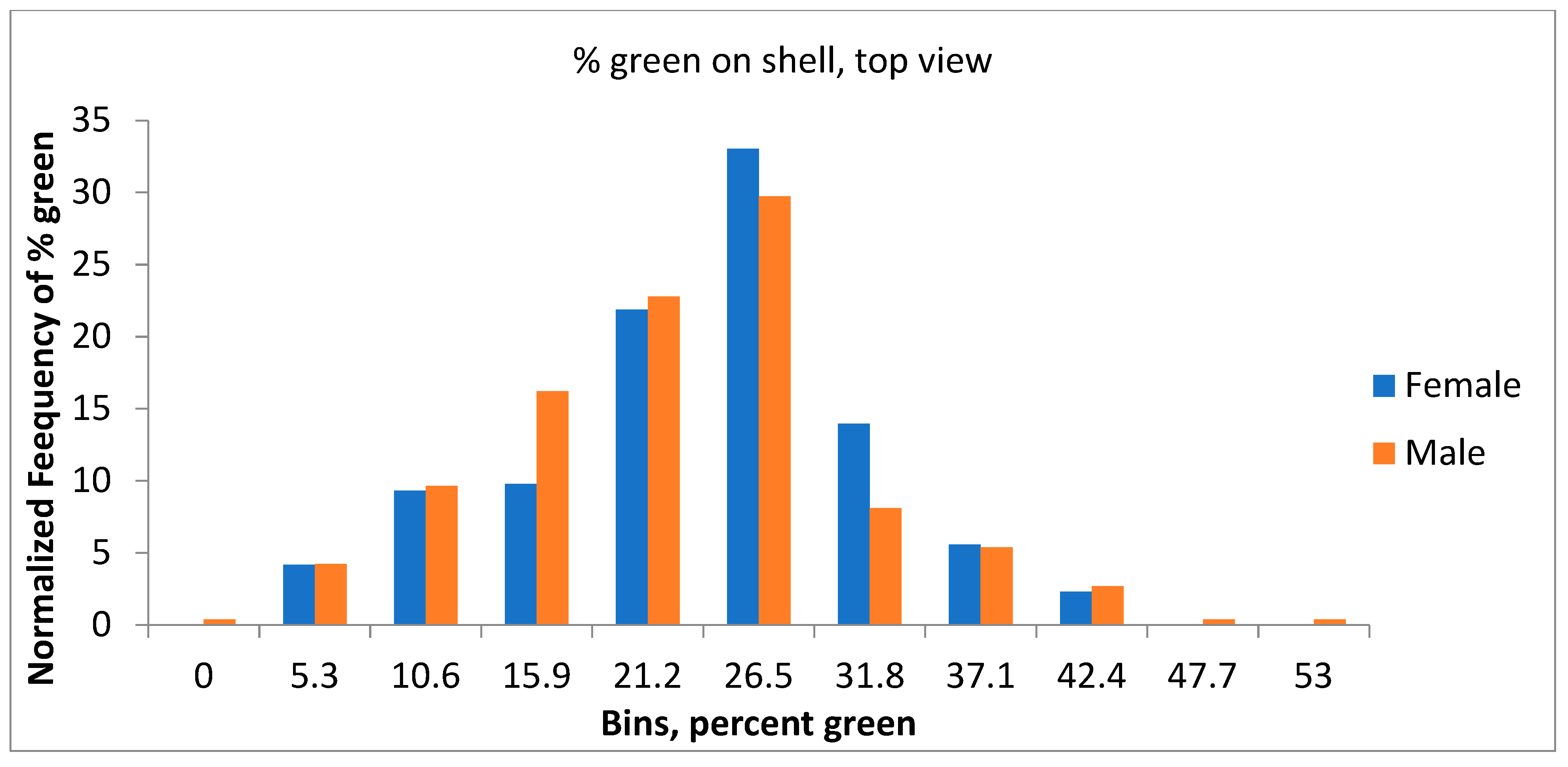
3.3. Results of Color Analysis

The average L*, a*, and b* of all the mussels, and females and males separately are given in

Table 5. Average color values of all of the mussels, female mussels, and male mussels.

	Average L*			Average a*			Average b*
	Overall	Female	Male	Overall	Female	Male	Overall	Female	Male
Average	45.79	45.64	45.92	0.97	0.76	1.15	14.99	14.72	15.22
St Dev	3.62	3.65	3.60	2.59	2.39	2.74	3.92	3.84	3.98
Min	36.86	36.94	36.86	−6.99	−4.77	−6.99	4.61	4.61	6.53
Max	57.09	56.74	57.09	11.5	6.91	11.5	29.04	28.74	29.04

St Dev: standard deviation of the averages presented.

. The histograms were constructed by first determining the maximum range of the parameter (e.g., L*) for both genders. Then, this range was divided by 10, resulting in 11 bins. Finally, the frequencies of the males were divided by the number of males, and those of the females were divided by the number of females to normalize the histograms. The histograms of the distributions of L* (Figure 4), a* (Figure 5), and b* (Figure 6) suggest that these color parameters are not different between genders. It is evident that the ranges of these color parameters are wide (as can be observed by the min and max values), the averages for females and males are close; the 95% confidence intervals overlap; and separation of gender by color alone is not possible. This conclusion is also confirmed by the results of t tests: for L* t stat = −0.814, p two tail = 0.416; for a* t stat = −1.635, p two tail = 0.103; and for b* t stat = −1.365, p two tail = 0.173.

The percentage of the shell top view area that is green was also measured. For this, the criterion of selecting green pixels as any pixel with an a* value < −5 was arbitrarily taken. In Figure 7, variation in the amount of green on the top view of the shell is displayed. In Figure 8, the histogram of the % green distribution for females and males is presented.

The yellow boundaries depict the areas where the above definition of green holds. It can be observed that there is wide variation. Also, there are mussels that exhibit very little or no green on their shell. The average % green is shown in Table 4 (around 20%). It is evident that the average % green values of females and males are not statistically different. Therefore, this parameter alone cannot be used to separate the mussels by gender.

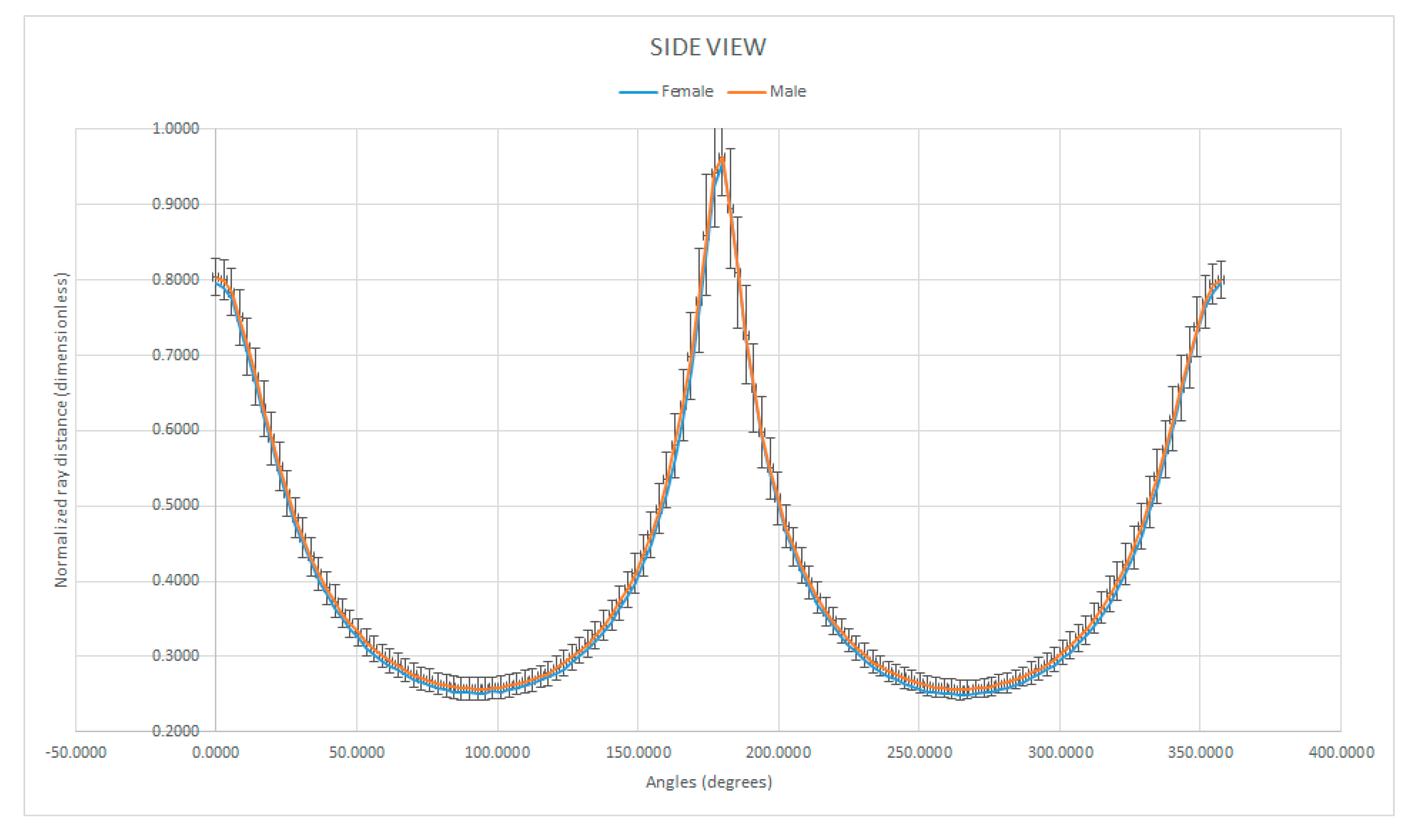
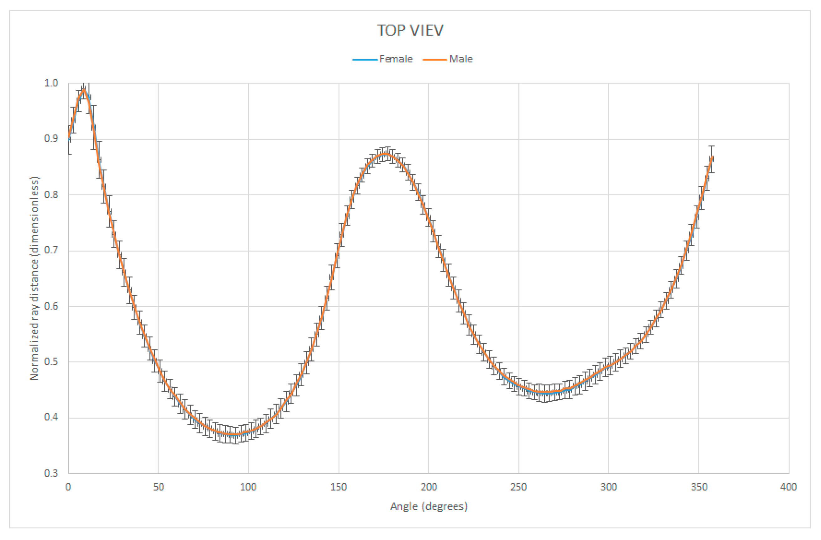
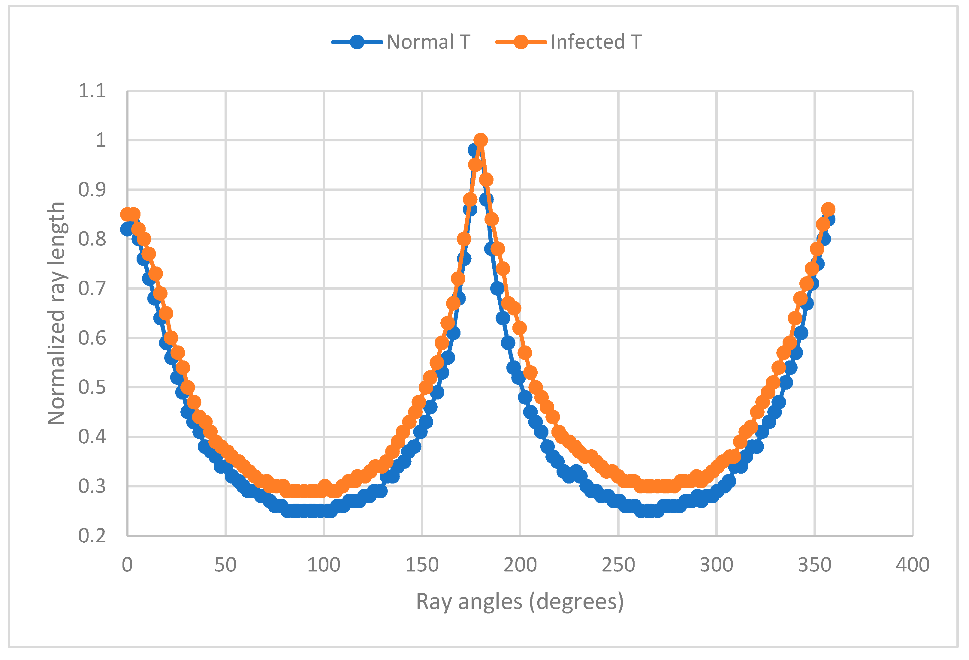
3.4. Shape Analysis by Normalized Ray Length vs. Ray Angle

Figure 9 presents the normalized ray lengths vs. ray angles for females and males for side view images. The standard deviation bars of males only were displayed so as not to crowd the plot. It is evident that females and males cannot be separated by using this method since their 95% confidence ranges overlap.

Figure 10 presents the normalized ray lengths vs. ray angles for females and males for top view images. Again, the standard deviation bars of males only were displayed so as not to crowd the plot. It is evident that the females and males cannot be separated by using this method since their 95% confidence ranges overlap.

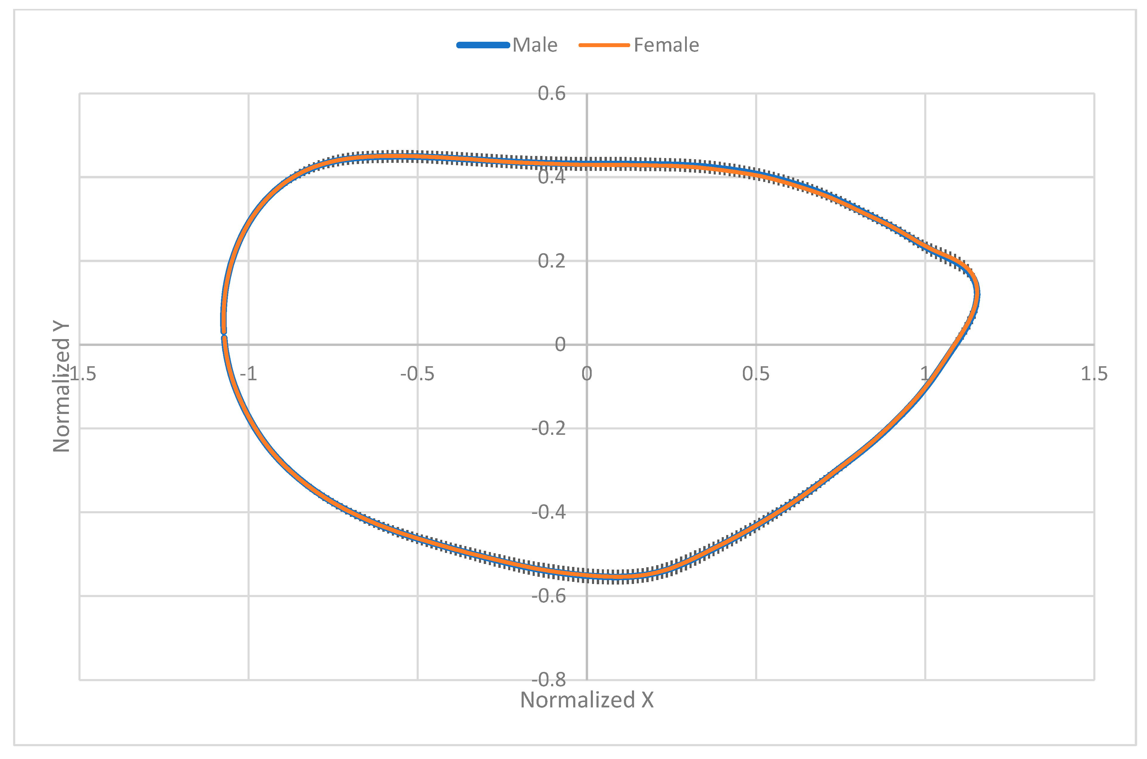
3.5. Results of Elliptic Fourier Analysis

The accuracy of the prediction of shape (X, Y points) by EFA depends on the number of harmonics used: the more harmonics included, the closer the predicted shape to the original shape. Analysis of the top view of 474 mussels by EFA revealed that the minimum critical harmonic was 6, and the maximum was 17 (Table 4). Therefore, up to and including the 25th harmonic was selected for the inclusion of parameters into statistical analysis. An example of the original perimeter and the predicted perimeter using the 25th harmonic for mussel 460 is shown in Figure 11. The critical harmonic for this mussel shape was the 17th harmonic. It is evident that taking the 25th harmonic for all mussels will result in the prediction of a good representation of the original shape.

The normalized predicted X Y values of the males and the females given by the 25th harmonic were averaged. This is a common method in EFA. Figure 12 presents the concurrent plot of these average values. The standard deviation of males only is shown so as not to crowd the plot. It can be observed that the males and females cannot be separated by using this method alone.

3.6. Artificial Neural Networks Analysis of EFA Shape Parameters

From the several neural networks tried, the best gender prediction had an error rate of 34.8%. It was, therefore, concluded that gender cannot be differentiated by using EPA normalized parameters in an artificial neural network.

3.7. PCA Analysis of EFA Shape Parameters

From inspection of the eigenvalues of the covariance matrix of the normalized EFA parameters, the number of principal components to explain 90% of the variation was calculated as 34. This implies a reduction in the number of independent variables from 97 to 34. However, no simple correlation could be found between these new independent variables to correctly predict the gender of mussels by shape.

3.8. Canonical Discriminant Analysis of EFA Shape Parameters

Cross-validation indicated the misclassification rate was 49%; very similar to what would be expected by chance (50%).

3.9. Random Forests Analysis of EFA Shape Parameters

The misclassification rate using this method was 49%; very similar to what would be expected by chance (50%).

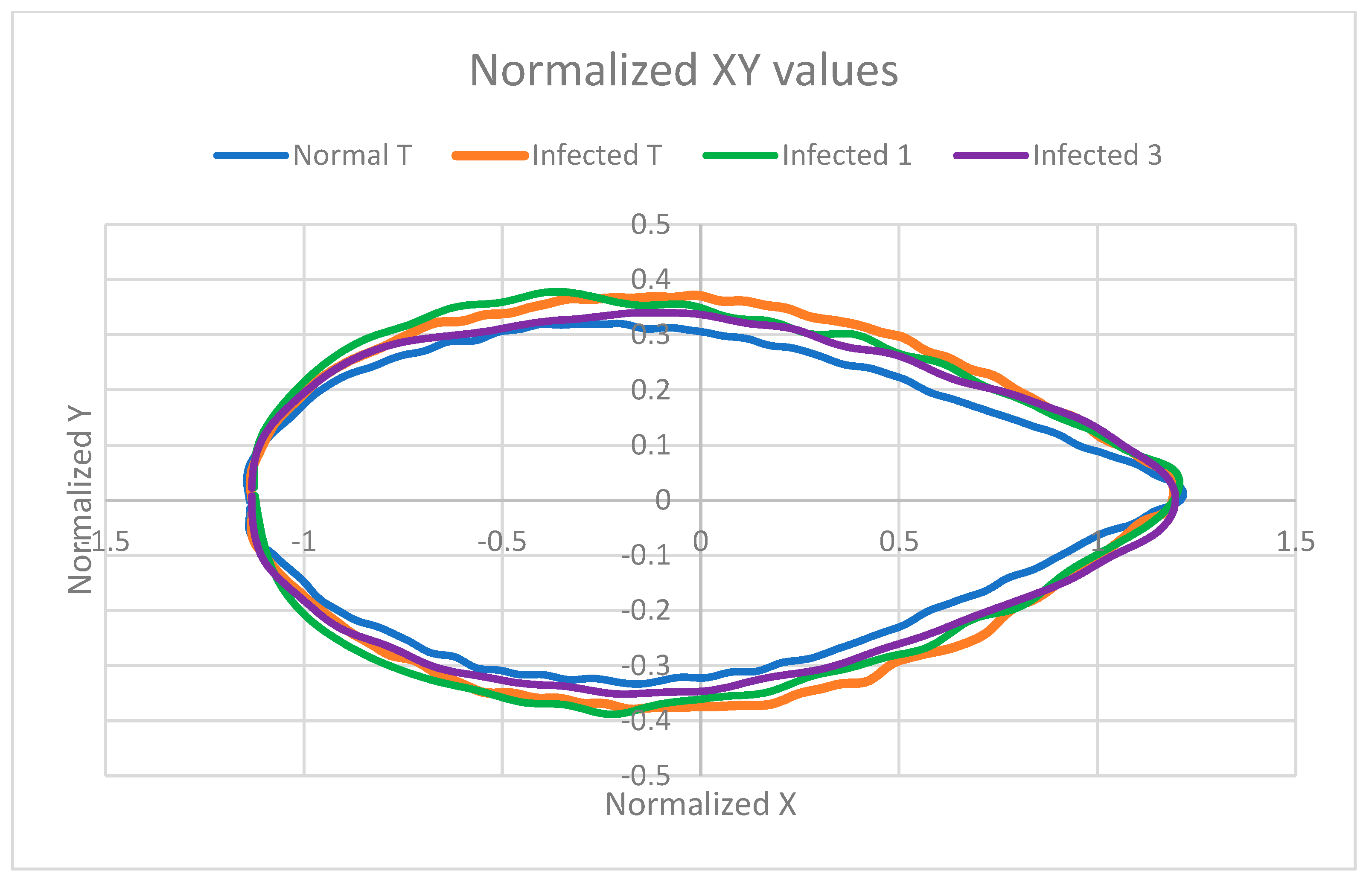
3.10. Effect of Pea Crab on Shape

New Zealand pea crab (N. novaezelandiae) is a parasite of green-lipped mussels [30]. Reported bivalve hosts of the crab are green-lipped mussel (Perna canaliculus), common blue mussel (Mytilus edulis), horse mussel (Atrina zelandica), and triangular trough shell (Crassula aequilater) [31]. In this study, only 4 mussels out of 474 contained pea crabs. Trottier [31] shows a picture of an uninfected and an infected mussel from the side, and mentions that the infection of pea crab results in measurable deleterious changes in the dimensions and growth of the mussel: mean shell height was significantly lower for infected mussels. Also, growth of length per day was 53% lower.

The image presented by Trottier [31] was analyzed by normalized ray length vs. ray angle (Figure 13). It is evident that there is a measurable shape difference. Also, the shapes in the same image were analyzed by EFA. The plot of the normalized X Y values for uninfected (normal T) and infected (infected T) mussels are shown in Figure 14. In addition, the results of two mussels infected by pea crab in this study were added to Figure 14. For these mussels, it is evident that the curves of all infected mussels are on the outside of the normal mussel. A statistical analysis was not performed with four infected mussels only, but the EFA may be a useful method to discriminate between infected and uninfected mussels.

4. Conclusions

The visual attributes (shape, size, and color) measured and analyzed by different methods did not result in a process to accurately differentiate between female and male unopened mussels. The existence of sexual dimorphism for this species is not mentioned in the literature. Since they were harvested from the same location and time, external factors’ impact on shape should be minimal. Regardless, the color, size, and shape data presented here should add to knowledge about the visual attributes of Greenshell^TM mussels, and will be valuable for future morphometric studies.

EFA–based shape analysis clearly differentiates between “intact” mussels and those with pea crabs. This method should be considered to locate mussels with parasite infection.

The mussels analyzed originated in the same location in November in New Zealand. Since location and time of year may have an effect on the results, this study should be repeated with mussels from different locations and harvested in different seasons, e.g., in May-June. Also, different mussel species should be tried.

References

1. Zhou, M. Comparison of Lipid Classes and Fatty Acid Profiles of Lipids from Raw, Steamed and High Pressure Treated New Zealand Greenshell™ Mussel Meat of Different Genders. Master’s Thesis, University of Auckland, Auckland, New Zealand, 2013. [Google Scholar]
2. MacDonald, G.A.; Hall, B.I.; Vlieg, P. Seasonal Changes in Proximate Composition and Glycogen Content of Greenshell™ Mussels; Mussel Industry Council Seminar, Crop & Food Research Ltd.: Nelson, New Zealand, 2000. [Google Scholar]
3. Sokolowski, A.; Bawazir, A.S.; Sokolowska, E.; Wolowicz, M. Seasonal variation in the reproductive activity, physiological condition and biochemical components of the brown mussel Perna perna from the coastal waters of Yemen (Gulf of Aden). Aquat. Living Resour. 2010, 23, 177–186. [Google Scholar] [CrossRef]
4. Zhou, M.; Balaban, M.O.; Gupta, S.; Fletcher, G. Comparison of lipid classes and fatty acid profiles of lipids from raw, steamed and high-pressure-treated New Zealand Greenshell™ mussel of different genders. J. Shellfish. Res. 2014, 33, 473–479. [Google Scholar] [CrossRef]
5. Aquaculture New Zealand. Available online: https://www.aquaculture.org.nz/news-article/aiformussels (accessed on 9 April 2025).
6. Zieritz, A.; Aldridge, D.C. Sexual, habitat-constrained and parasite-induced dimorphism in the shell of a freshwater mussel (A. anatine, Unionidae). J. Morphol. 2011, 272, 1365–1375. [Google Scholar] [CrossRef]
7. Kotrla, M.B.; James, F.C. Sexual dimorphism of shell shape and growth of Villosa villosa (Wright) and Elliptio icterina (Conrad) (Bivalvia: Unioidae). J. Molloscan Stud. 1987, 53, 13–23. [Google Scholar] [CrossRef]
8. Trivellini, M.M.; Van der Molen, S.; Márquez, F. Fluctuating asymmetry in the shell shape of the Atlantic Patagonian mussel, Mytilus platensis, generated by habitat-specific constraints. Hydrobiologia 2018, 822, 189–201. [Google Scholar] [CrossRef]
9. Steffani, C.N.; Branch, G.M. Growth rate, condition, and shell shape of Mytilus galloprovincialis: Response to wave exposure. Mar. Ecol. Prog. Ser. 2003, 246, 197–209. [Google Scholar] [CrossRef]
10. Reimer, O.; Tedengren, M. Phenotypical improvement of morphological defenses in the mussel Mytilus edulis induced by exposure to the predator Asterias rubens. Oikos 1996, 75, 383–390. [Google Scholar] [CrossRef]
11. Telesca, L.; Michalek, K.; Sanders, T.; Peck, L.S.; Thyrring, J.; Harper, E.M. Blue mussel shell shape plasticity and natural environments: A quantitative approach. Sci. Rep. 2018, 8, 2865. [Google Scholar] [CrossRef]
12. Hickman, R.W. Allometry and growth of the green-lipped mussel Perna canaliculus in New Zealand. Mar. Biol. 1979, 51, 311–327. [Google Scholar] [CrossRef]
13. Thejasvi, A.; Shenoy, C.; Thippeswamy, S. Morphometric and length-weight relationships of the green mussel Perna viridis (Linnaeus) from a subtidal habitat of Karwar coas, Karnataka, India. Int. J. Recent Sci. Res. 2014, 5, 295–299. [Google Scholar]
14. Alcicek, Z.; Balaban, M.O. Estimation of whole volume of green shelled mussels using their geometric attributes obtained from image analysis. Int. J. Food Prop. 2014, 17, 1987–1997. [Google Scholar] [CrossRef]
15. Balaban, M.O.; MChombeau Cırban, D.; Gümüş, B. Prediction of the weight of Alaskan pollock using image analysis. J. Food Sci. 2010, 75, E552–E556. [Google Scholar] [CrossRef] [PubMed]
16. Dommergues, E.; Dommergues, J.L.; Magniez, F.; Neige, P.; Varrechia, E.P. Geometric measurement analysis versus Fourier series analysis for shape characterization using the gastropod shell (Trivia) as an example. Math. Geol. 2003, 35, 887–894. [Google Scholar] [CrossRef]
17. Balaban, M.; Odabasi, A.Z. Measuring color with machine vision. Food Technol. 2006, 60, 32–36. [Google Scholar]
18. Zahn, C.; Roskies, R.R. Fourier descriptors for plane closed curves. IEEE Trans Comput. 1972, C-21, 269–281. [Google Scholar] [CrossRef]
19. Costa, C.; Aguzzi, J.; Menesatti, P.; Antonucci, F.; Rimatori, V.; Mattoccia, M. Shape analysis of different poulations of clams in relation to their geographical structure. J. Zool. 2008, 276, 71–80. [Google Scholar] [CrossRef]
20. Palmer, M.; Pons, G.X.; Linde, M. Discriminating between geographical groups of a Mediterranean commercial clam (Chamelea gallina L. Veneridae) by shape analysis. Fish. Res. 2004, 67, 93–98. [Google Scholar] [CrossRef]
21. Rufino, M.M.; Gaspar, M.B.; Pereira, A.M.; Vasconcelos, P. Use of shape to distinguish Chamelea gallina and Chamelea striatula (Bivalvia: Veneridae): Linear and geometric morphometric methods. J. Morphol. 2006, 267, 1433–1440. [Google Scholar] [CrossRef]
22. Costa, C.; Menesatti, P.; Aguzzi, J.; D’Andrea, S.; Antonucci, F.; Rimatori, V.; Pallottino, F.; Mattocia, M. External shape differences between Sympatric populations of commercial clams Tapes decussatus and T. philippinarum. Food Bioprocess Technol. 2010, 3, 43–48. [Google Scholar] [CrossRef]
23. Marquez, F.; Van der Molen, S. Intraspecific shell shape variation in the razor clam Ensis macha along the Patagonian coast. J. Molluscan Stud. 2011, 77, 123–130. [Google Scholar] [CrossRef]
24. Preston, S.J.; Harrison, A.; Lundy, M.; Roberts, D.; Beddoe, N.; Rogowski, D. Square pegs in round holes—The implications of shell shape variation on the translocation of adult Margaritifera margaritifera (L.). Aquat. Conserv. Mar. Freshw. Ecosyst. 2010, 20, 568–573. [Google Scholar] [CrossRef]
25. Luzuriaga, D.; Balaban, M.O.; Yeralan, S. Analysis of visual quality attributes of white shrimp by machine vision. J. Food Sci. 1997, 62, 113–118. [Google Scholar] [CrossRef]
26. Leyva-Valencia, I.; Alvarez-Castaneda, S.T.; Lluch-Cota, D.B.; Onzalez-Pelaez, S.; Perez-Valencia, S.; Vadopalas, B.; Ramirez-Perez, S.; Cruz-Hernandez, P. Shell shape differences between two Panopea species and phenotypic variation among P. globose at different sites using two geometric morphometric approaches. Malacologia 2012, 55, 1–13. [Google Scholar] [CrossRef]
27. Ninomiya, S.; Ohsawa, R.; Yoshida, M. Evaluation of buckwheat and tartary buckwheat kernel shape by elliptic Fourier method. Curr. Adv. Buckwheat Res. 1995, 389–396. [Google Scholar]
28. MacLeod, N. (Nanjing University, Nanjing, China). Personal communication, 2020.
29. Gumus, B.; Balaban, M.O. Prediction of the weight of aquacultured rainbow trout (Oncorhynchus mykiss) by image analysis. J. Aquatic Food Prod. Technol. 2010, 19, 227–237. [Google Scholar] [CrossRef]
30. Hickman, R.W. Incidence of pea crab and a trematode in cultivated and natural green-lipped mussels. N. Z. J. Mar. Freshw. Res. 1978, 12, 211–215. [Google Scholar] [CrossRef]
31. Trottier, O.J. Biology and Impact of the New Zealand Pea Crab (Nepinnotheres novaezelandiae) in Aquacultured Green Lipped Mussels (Perna canaliculus). Ph.D. Thesis, University of Auckland, Auckland, New Zealand, 2014. [Google Scholar]
Figure 2. Image analysis of mussels for dimensions and shape. (a): Original picture; (b): fitted best rectangle to measure length, width, and height; (c): determination of ray angle and normalized ray length for shape analysis. CG = center of gravity.
Fishes 10 00325 g002
Figure 3. Top: Calculated power curve for height vs. average length of female and male mussels. Bottom: Calculated height/length vs. width/length for female and male mussels. nmales = 259, nfemales = 215.
Fishes 10 00325 g003aFishes 10 00325 g003b
Figure 4. Normalized histogram of average L* values for female and male mussels. nmales = 259, nfemales = 215.
Fishes 10 00325 g004
Figure 5. Normalized histogram of average a* values for female and male mussels. nmales = 259, nfemales = 215.
Fishes 10 00325 g005
Figure 6. Normalized histogram of average b* values for female and male mussels. nmales = 259, nfemales = 215.
Fishes 10 00325 g006
Figure 7. Examples of percent green on the view area of mussels. a* < −5.
Fishes 10 00325 g007
Figure 8. Normalized histogram of % green for females and males. nmales = 259, nfemales = 215.
Fishes 10 00325 g008
Figure 9. Shape analysis using average ray lengths vs. ray angles for females and males. Side view. nmales = 259, nfemales = 215.
Fishes 10 00325 g009
Figure 10. Average normalized ray distances vs. average angles (degrees). Top view of shells. nmales = 259, nfemales = 215.
Fishes 10 00325 g010
Figure 11. Shape analysis using EFA. Top: Selection of the harmonic to calculate X Y values. The original perimeter and the X Y values using the 25th harmonic for a mussel for which the % perimeter error becomes less than 1% at harmonic 17.
Fishes 10 00325 g011
Figure 12. Plot of average normalized X Y values for females and males. Only the standard deviation of males shown. nmales = 259, nfemales = 215.
Fishes 10 00325 g012
Figure 13. Effect of pea crab infection on shape analyzed by EFA. Difference in the normalized ray length vs. normalized ray angle for the side view. Image for analysis taken from Trottier (2014).
Fishes 10 00325 g013
Figure 14. Normalized EFA plot for a normal mussel and three infected mussels. Names ending with T are results of analysis using an image taken from [31]. Others are from this study.
Fishes 10 00325 g014