Article

FishSegNet-PRL: A Lightweight Model for High-Precision Fish Instance Segmentation and Feeding Intensity Quantification

1
Key Laboratory of Fisheries Remote Sensing, Ministry of Agriculture and Rural Affairs, East China Sea Fisheries Research Institute, Chinese Academy of Fishery Sciences, Shanghai 200090, China
2
College of Navigation and Ship Engineering, Dalian Ocean University, Dalian 116023, China
3
Shenzhen Shengya Environment Technology Ltd., Shenzhen 518000, China
4
Guangzhou Nansha Fishery Industry Park Co., Ltd., Guangzhou 510000, China
*
Authors to whom correspondence should be addressed.
Fishes 2025, 10(12), 630; https://doi.org/10.3390/fishes10120630
Submission received: 3 November 2025 / Revised: 27 November 2025 / Accepted: 4 December 2025 / Published: 9 December 2025
(This article belongs to the Special Issue Biodiversity and Spatial Distribution of Fishes, Second Edition)

Abstract

Siniperca chuatsi, commonly known as mandarin fish, is one of the most economically valuable freshwater species in China. In 2022, the national aquaculture production of mandarin fish reached approximately 401,000 tons, accounting for a significant share of freshwater aquaculture in China and nearly dominating the global commercial farming landscape. With the rapid development of recirculating aquaculture systems (RASs), higher requirements have been raised for feeding efficiency and fish health monitoring. Traditional on-site visual observation methods are highly subjective, inefficient, difficult to quantify, and prone to misjudgment under conditions such as insufficient illumination, turbid water, or high stocking density. To address these challenges, this study proposes FishSegNet-PRL, an instance segmentation-based model designed to quantify the feeding intensity of mandarin fish. The model is built upon the YOLOv11-seg framework, enhanced with a P2 detection layer (P), a residual cross-stage spatial–channel attention module (RCSOSA, R), and a lightweight semantic-detail-enhanced cascaded decoder (LSDECD, L). These improvements collectively enhance small-target detection capability, boundary segmentation accuracy, and real-time inference performance. Experimental results demonstrate that FishSegNet-PRL achieves superior performance in mandarin fish instance segmentation, with a Box mAP50 of 85.7% and a Mask mAP50 of 79.4%, representing improvements of approximately 4.6% and 13.2%, respectively, compared with the baseline YOLOv11-seg model. At the application level, multiple feeding intensity quantification indices were constructed based on the segmentation results and evaluated, achieving a temporal intersection-over-union (IoUtime) of 95.9%. Overall, this approach enables objective and fine-grained assessment of mandarin fish feeding behavior, striking an effective balance between accuracy and real-time performance. It provides a feasible and efficient technical solution for intelligent feeding and behavioral monitoring in aquaculture.
Key Contribution: A lightweight model, FishSegNet-PRL, is proposed for precise fish segmentation and quantitative feeding-intensity assessment in aquaculture.

1. Introduction

With the continuous growth of the global population and the rising demand for aquatic products, aquaculture is playing an increasingly prominent role in global food supply. According to the FAO report, the total global aquatic production (capture fisheries + aquaculture) reached approximately 223.2 million tons in 2022, representing a 4.4% increase compared with 2020. Notably, for the first time, the production of farmed aquatic animals surpassed that of traditional capture fisheries, underscoring the dominant position of aquaculture in the global aquatic food supply [1,2]. In China, the aquaculture production of mandarin fish (Siniperca chuatsi) reached approximately 401,000 tons in 2022, accounting for a substantial share of the nation’s freshwater aquaculture and exerting a significant influence on the global commercial farming landscape [3]. In intensive recirculating aquaculture systems (RASs), a key challenge for improving efficiency and sustainability lies in achieving higher yields with reduced feed input while ensuring both fish growth and environmental health. Traditional experience-based feeding practices are easily influenced by factors such as variations in light conditions, water turbidity, surface disturbances, and crowding, which may lead to subjective misjudgments, feed wastage, and consequently increased pressure on water quality [4,5]. Consequently, precise feeding and behavioral monitoring have been increasingly recognized as essential technological pathways to enhance feed utilization and improve aquaculture performance [6,7].
In recent years, the rapid progress of deep learning has established a new technological paradigm for precision aquaculture through visual computing and multimodal perception, with applications spanning fish detection and counting, health monitoring, intelligent feeding, and water quality prediction [8]. Fish behavior analysis is particularly critical for intelligent feeding. Feeding behavior not only directly reflects the fish’s response to feed but also serves as an indicator of external factors such as water quality, health status, or psychological state. Current studies have mainly focused on computer vision, acoustics, and sensor-based approaches, and have highlighted that multimodal fusion and spatiotemporal graph modeling can significantly enhance robustness and interpretability [9]. Fish feeding behavior provides external cues including water quality, psychological state, and feeding intensity. Therefore, effectively analyzing feeding behavior is a core step in determining fish feeding intensity.
In aquaculture, computer vision has attracted considerable attention as a non-invasive approach for quantifying fish feeding intensity. Related studies have mainly focused on three directions: object detection and tracking, instance segmentation, and object recognition with behavior classification. A large body of work has characterized the dynamics of fish feeding behavior through object detection combined with multi-object tracking. These methods typically extract trajectory features such as velocity, acceleration, and turning rate to classify feeding intensity levels. Zhao et al. [10] integrated improved ByteTrack-based multi-fish tracking with a spatiotemporal graph convolutional network (ST-GCN), enabling relatively accurate recognition of different feeding levels. Huang et al. [11] constructed a benchmark dataset for real-time multi-fish tracking in aquaculture scenarios and proposed a cross-scale content-adaptive network to mitigate issues of high density and occlusion, thereby providing a foundation for stable feeding intensity quantification. In addition, Li et al. [12] enhanced DeepSORT by incorporating DCNv2 and attention mechanisms, maintaining trajectory integrity even under low-light and turbid underwater conditions. Furthermore, Zhao et al. [13] proposed the FishFeed system, which replaces individual trajectories with variations in fish density distribution to enable real-time feeding decisions. Nevertheless, such detection- and tracking-based approaches still face limitations under conditions of severe occlusion and high stocking density.
To address the limitations of individual tracking, which often fails to remain stable in dense scenarios, researchers have shifted toward instance or semantic segmentation methods, using group-level spatial structures and geometric features as the basis for feeding intensity quantification. Yang et al. [14] proposed FSFS-Net, which achieves more robust segmentation under highly aggregated and overlapping fish schools, thereby providing reliable data for extracting spatial features of feeding intensity. Wang et al. [15] combined VoVNetv2 with Shuffle Attention to effectively reduce edge segmentation errors caused by lighting variations and bubbles. Similarly, Yang et al. [16] employed a BlendMask-VoVNetV2 framework to accurately segment and quantify fish numbers and areas, supporting more objective evaluation of intensity levels. In addition, Kong et al. [17] demonstrated the potential of semantic segmentation for high-precision feeding, utilizing the characterization of aggregation and dispersion dynamics to facilitate automated feeding decisions. These findings indicate that instance segmentation methods can effectively circumvent the challenges of individual tracking in complex environments, thereby improving the operability of feeding intensity quantification.
In subsequent developments, research has increasingly regarded feeding intensity as a spatio-temporal recognition and multimodal fusion problem, aiming to overcome the limitations of single-frame images or single features in comprehensively capturing feeding dynamics. Ubina et al. [18] employed a two-stream optical flow network combined with a 3D CNN to effectively capture dynamic textures and motion patterns in feeding behavior. Feng et al. [19] proposed 3D ResNet-Glore, which enabled real-time intensity quantification. Similarly, Zhang et al. [20] integrated Mo-bileNetV2 with SENet to accurately distinguish four feeding intensity levels (“none, weak, moderate, strong”) under complex lighting and reflection conditions. To mitigate interference from surface reflections, Wu et al. [21] developed a recognition method based on the appearance and dynamic features of “feeding splashes,” demonstrating strong robustness in outdoor pond environments. Moreover, Wei et al. [22] introduced an improved kinetic model combined with a graph convolutional network, explicitly incorporating temporal sequence learning to characterize the dynamic evolution of the entire feeding process. In recent years, a trend toward multimodal fusion has also emerged. For instance, Dong et al. [23] proposed a three-stream network, while Li et al. [24] introduced an audio–visual complementary method, both of which improved recognition accuracy under complex water conditions and advanced toward ten-level continuous scoring and closed-loop feeding control. Overall, this stage of research has moved beyond the constraints of unimodal and static analysis, emphasizing spatiotemporal consistency and multimodal integration, thereby providing new support for intelligent feeding.
Although substantial progress has been made in quantifying fish feeding intensity, several critical limitations remain in real-world intensive recirculating aquaculture environments. Under conditions of occlusion, overlap, and high-density fish schools, the accuracy of detecting and segmenting small individuals decreases significantly [25]. Segmentation models such as FSFS-Net have improved group structure representation under occlusion and aggregation; however, their performance metrics (e.g., mIoU) still show notable degradation when fish fully cover the field of view, when illumination varies considerably, or under turbid water conditions [14]. Existing methods also lack sufficient continuity in temporal characterization. Most studies classify feeding intensity only at specific stages of feeding (e.g., initiation or peak) or from static frames, while failing to capture the dynamic trend of the entire feeding process from onset to decline. This limits their potential for early warning or real-time adjustment of feeding strategies. In addition, segmentation of fish body edges and fine details (such as fins and tails) often remains imprecise. Combined with large model sizes and complex architectures, such methods impose high computational demands, making real-time deployment on edge devices or in aquaculture facilities challenging [26]. Therefore, it is still necessary to explore more efficient and interpretable modeling approaches.
This study reconsiders the quantification of fish feeding intensity from a novel perspective and proposes the FishSegNet-PRL instance segmentation method to learn the correlations among different semantic features. A series of interpretable spatial behavioral sequence indices—such as total area and nearest-neighbor distance—are defined and computed. Feeding intensity levels are then classified according to differences in image representations under varying conditions, including degrees of aggregation, occlusion, and overlap. Finally, the FishSegNet-PRL algorithm is validated on video datasets representing four feeding intensity levels (none, weak, moderate, strong). By performing instance segmentation on video frames to extract spatial features and applying a LightGBM model for feeding intensity prediction, the method outputs either continuous intensity values or categorical classifications. The main contributions of this study are as follows:
  • We propose the FishSegNet-PRL instance segmentation method, which is capable of extracting multiple key feature indices—including total area, nearest-neighbor distance, area growth rate, cluster number, and perimeter-to-area ratio—to comprehensively characterize the spatial structural behavior of fish schools.
  • We construct a fish instance segmentation dataset covering diverse feeding image conditions (e.g., occlusion, overlap, and aggregation), which is used to train and evaluate models for extracting spatial structural behavioral features.
  • We experimentally validate the effectiveness of FishSegNet-PRL on video datasets annotated with four feeding intensity levels (none, weak, moderate, strong). Using the spatial behavioral features extracted by FishSegNet-PRL as inputs, the LightGBM model enables fine-grained classification and continuous prediction of feeding intensity, thereby achieving quantitative representation of feeding dynamics.

2. Materials and Methods

Quantification of fish school feeding behavior is a critical component of intelligent feeding. To achieve this objective, we collected and annotated a mandarin fish (Siniperca chuatsi) feeding behavior dataset under intensive recirculating aquaculture conditions, using a single semantic class (“fish”) for instance-level annotation. The dataset covers the entire feeding cycle, including pre-feeding, feeding, and post-feeding stages. Based on this dataset, we propose the FishSegNet-PRL model to perform fish instance segmentation. From the segmentation masks, a set of spatial behavioral indices—including fish pixel area ratio, nearest-neighbor distance, cluster number, area growth rate, and perimeter-to-area ratio—were constructed and calculated. These indices were then compared across four feeding intensity levels (“none,” “weak,” “moderate,” and “strong”) using video clips. Finally, the extracted features were input into a LightGBM model for quantitative prediction of feeding intensity, enabling both continuous value estimation and categorical classification. The framework for quantifying mandarin fish feeding behavior is illustrated in Figure 1.

2.1. Data Acquisition and Dataset Split

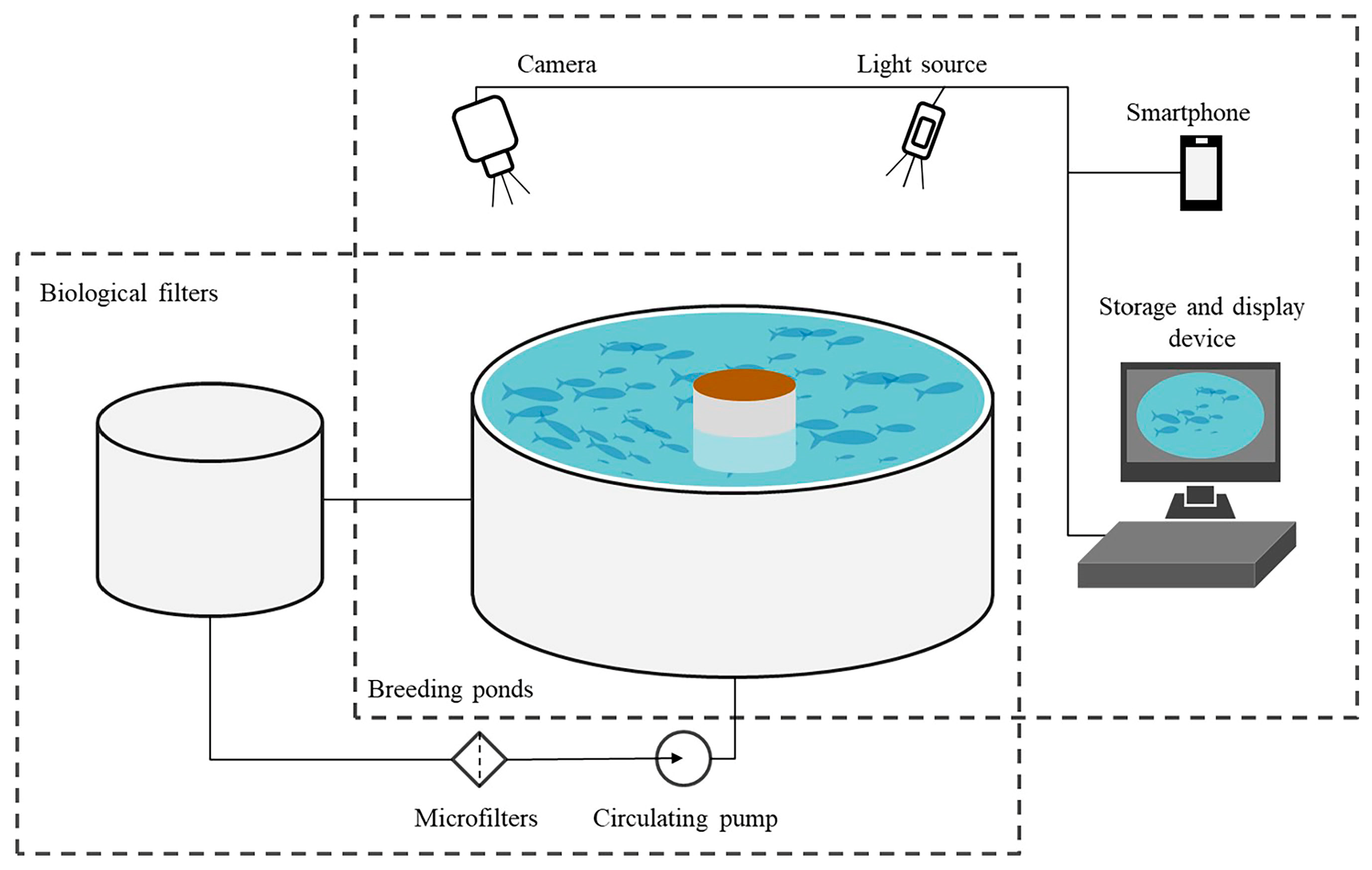
This study focuses on the mandarin fish (Siniperca chuatsi) in a recirculating aquaculture system (RAS). All video data were collected from the Nansha Fishery RAS facility between 1 June and 31 August 2024. The facility uses 200 m2 stainless steel tanks, each stocked at a density of approximately 50 kg/m3, maintaining stable water quality with dissolved oxygen ≥ 8 mg/L. A microfiltration + biochemical treatment system ensures water quality. Data were collected from standard circular tanks C7, C8, and C10, with feeding behavior data covering two high-activity periods in the early morning and evening to capture the full “pre-feeding, feeding, and post-feeding” behavior sequences. The data collection system used a Hikvision high-definition industrial camera (1920 × 1080, 30 fps), mounted vertically above the tanks on a waterproof bracket about 400 mm above the water surface, with fixed focal length and exposure. The recirculating aquaculture system diagram is shown in Figure 2.
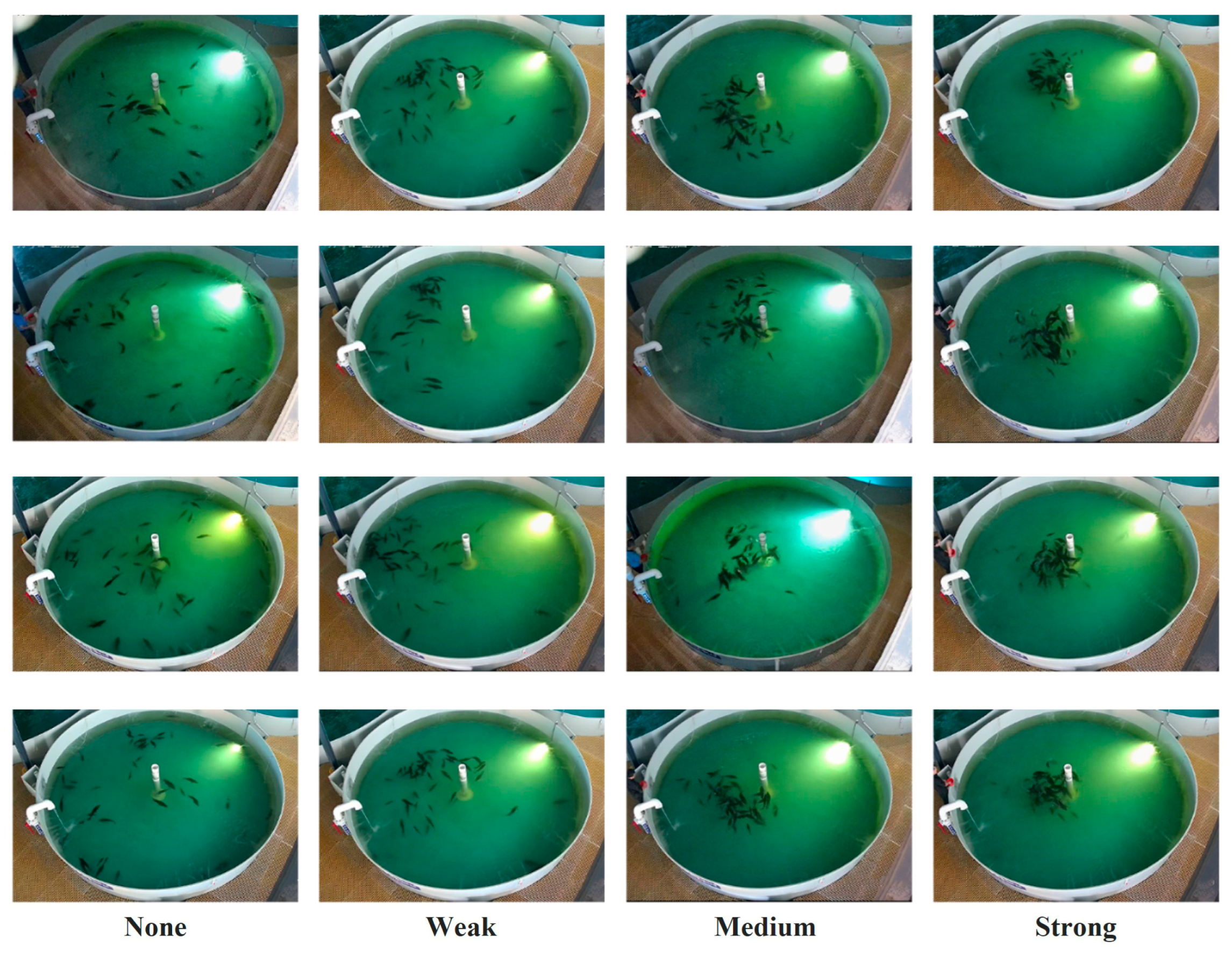
To capture fish school phenotypes under different behavioral states, four feeding intensity levels were defined in this study: strong, medium, weak, and none, as illustrated in Figure 3. Specifically, under comparable stocking densities, feeding intensity levels were manipulated by adjusting feed quantities and feeding times, ensuring that all four levels were represented within the same environmental conditions and time windows. Ultimately, six video clips (each lasting 5–7 min) were selected from the raw monitoring footage collected at the aquaculture facility. Each clip encompassed continuous sequences covering the pre-feeding, feeding, and post-feeding stages, while segments with abnormal lighting, strong glare, or significant focus failures were excluded to ensure representativeness and usability of the samples. A summary of feeding activity records is provided in Table 1. The detailed descriptions of the different feeding intensity levels are as follows:
Strong feeding: During feeding, fish may exhibit aggregation behavior due to competition for food, with a large number of splashes occurring within a short period of time. Individual fish in the images often display pronounced overlap and occlusion.
Medium feeding: After feeding for a certain period, fish may continue to aggregate temporarily, possibly because they have not yet obtained sufficient food. The aggregation lasts longer, the range of aggregation expands, and a moderate number of splashes are observed within a short time. Partial overlap and occlusion among fish are also present.
Weak feeding and no feeding: Following feeding, fish reject the feed and swim away from the feeding area, leading to a broader distribution range. Only a few splashes appear, which may result from minor movements of individual fish. In this context, weak feeding corresponds to the basic state when fish cease active feeding, whereas after an extended period the school disperses into the no-feeding state. Thus, both weak feeding and no feeding serve as indicators of feeding termination.
The video preprocessing and segmentation are performed on the saved video data through playback processing. To balance temporal redundancy and sample diversity, this study uniformly sampled frames from the original 30 fps monitoring video by selecting every 5th frame, resulting in an image sequence with an effective frame rate of 6 fps. During data extraction, the experimental fish school remained in the same recirculating aquaculture system, and the number of individuals did not change due to factors such as death or harvesting. Subsequently, the sampled images were manually annotated using the Image Recognition feature of the makesense annotation platform, classifying each frame into four feeding intensity levels: “strong,” “medium,” “weak,” and “none.” A total of 1400 images with intensity labels were obtained and used as ground truth data for the LightGBM model. These ground truth labels, along with spatial quantitative metrics (such as fish pixel area, nearest-neighbor distance, etc.) derived from the instance segmentation results, together form the feature-label dataset for LightGBM. The dataset was split into training, testing, and validation sets at a ratio of 8:1:1, to train the LightGBM model and learn the quantitative calculation method for feeding intensity.
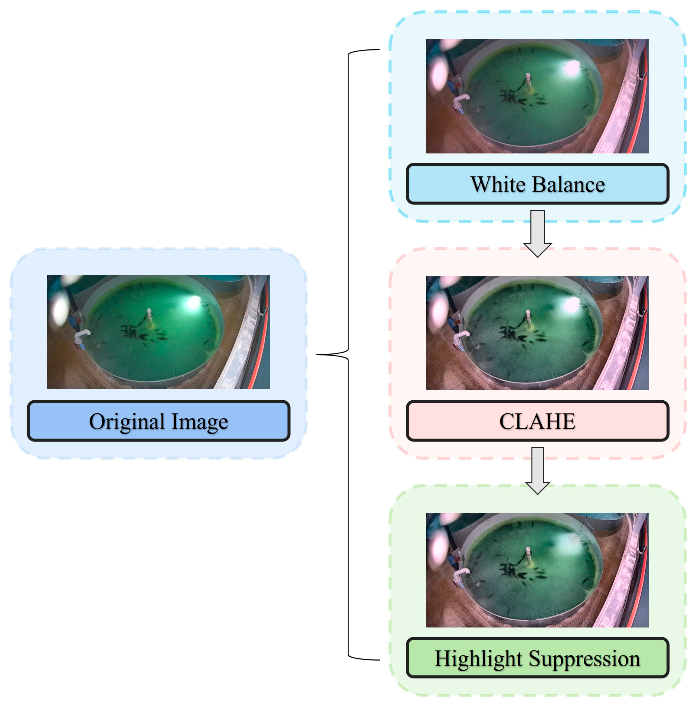
During the data collection process, factors such as the greenish tint of the water, localized strong reflections or glare (from spotlights and specular reflections on the water surface), water turbidity, bubbles, and texture reflections from the tank walls and floor led to a significant reduction in contrast between the fish and the background during certain periods. Additionally, the mandarin fish has a highly similar appearance and color, and during feeding, there is often high-density aggregation, mutual occlusion, and rapid movement, leading to motion blur, boundary adhesion, fin loss, and missed detection of small individuals. To improve image quality and enhance the accuracy of subsequent segmentation, this study employed image enhancement techniques such as white balance correction, CLAHE, and highlight suppression: First, to address the greenish tint of the water, the white balance adjustment was made by setting the color temperature coefficients for the RGB channel gains to 0.9 and 0.85, effectively correcting the overall color bias and eliminating the greenish tint in the underwater images [27]; next, to enhance low-contrast areas, the clip limit for CLAHE was set to 2.0, and the tile grid size was set to 16 × 16, optimizing the local contrast of the image, enhancing details in dark and mid-to-low contrast regions, improving the visibility of small targets, and avoiding the introduction of excessive noise [28]; finally, to suppress the pseudo-foreground caused by strong reflections, highlight suppression was applied with a suppression strength of 0.6 and a suppression range of 40 pixels, effectively smoothing the high-glare areas on the water surface, reducing reflections and timestamps, and improving the separability between the fish and the background [29]. These preprocessing steps significantly improved the clarity of the image contours and the visibility of small targets, reduced the interference of reflections and pseudo-foregrounds, and provided a more stable training environment for subsequent instance segmentation, thereby enhancing the model’s robustness and generalization ability. The preprocessing workflow is shown in Figure 4.
To ensure consistency with subsequent instance segmentation and spatial metric calculations, the number of fish in the school remained constant during dataset extraction and was not affected by factors such as death or harvesting. In this study, the target annotation was based on a single semantic class, ‘fish,’ and the annotation was manually performed using the polygon instance contour labeling method in the ISAT v1.3.5 (Image Segmentation Annotation Tool). The specific rules are as follows:
Separable individuals: Fish with clear contours and distinguishable boundaries were independently annotated as separate instances, labeled as fish.
Severe adhesion: When the boundaries of two or more individuals could not be reliably separated, they were annotated as a single fish instance based on the overall identifiable outline.
Non-target exclusion: Splashes, bubbles, feed particles, reflections, and shadows were excluded from annotation.
A total of 1400 images with mandarin fish targets and 25,567 annotated instances were obtained for instance segmentation using the FishSegNet-PRL model. To ensure the effectiveness of model training, the dataset was split into training, testing, and validation sets at a ratio of 8:1:1. These were used to calculate and compare spatial quantitative indices (e.g., fish pixel area, nearest-neighbor distance) across different feeding intensities, thereby supporting subsequent feeding intensity quantification and graded evaluation.

2.2. Instance Segmentation Model: FishSegNet-PRL

In this study, we address the problem of instance segmentation of mandarin fish (Siniperca chuatsi) feeding images in overhead circular tank scenarios and propose FishSegNet-PRL to tackle practical challenges such as dense fish schools, small targets, missing edge details, and strong reflection interference. In the preprocessing stage, white balance correction was applied to eliminate green bias in the water, CLAHE was employed to enhance details in dark and mid-to-low contrast regions, and highlight suppression was introduced to reduce the impact of specular reflections and pseudo-foregrounds on segmentation. In addition, mildly deblurring and sharpening were performed on motion-blurred frames to restore edge information. Based on this, the network architecture was enhanced with a P2 detection layer to incorporate high-resolution shallow features into detection, thereby improving the recall of fins, small individuals, and densely packed fish. At the neck stage, the RCSOSA module was adopted, integrating residual connections with channel–spatial attention, and combining multi-branch training with re-parameterization during inference to preserve edge and detail information in complex backgrounds. For the segmentation head, a lightweight LSDECD was introduced for dense context modeling, enhancing the representation of texture and contour details. With these improvements, the model can efficiently perform instance segmentation of mandarin fish feeding images and provide reliable support for feeding intensity quantification. For quantification, feeding intensity was assessed based on instance segmentation results and behavioral features, with hyperparameter tuning conducted using the LightGBM algorithm. Finally, the proposed method was evaluated for both instance segmentation and feeding intensity quantification of mandarin fish, demonstrating its feasibility and accuracy.

2.2.1. Overall Architecture of the FishSegNet-PRL Model

In feeding images from mandarin fish (Siniperca chuatsi) aquaculture scenarios, challenges commonly arise due to complex lighting conditions, variable water backgrounds, frequent occlusion among individuals, and significant differences in fish body sizes. The dataset collected in this study also exhibits these typical characteristics. Under such conditions, directly applying the baseline YOLOv11-seg model for instance segmentation often fails to achieve satisfactory results; simply enlarging the model may improve accuracy but at the cost of substantially increased computational and storage overhead, which hinders real-time deployment in aquaculture settings. To address these issues, this study adopts YOLOv11-seg as the backbone framework and introduces targeted improvements tailored to the requirements of mandarin fish feeding intensity quantification:
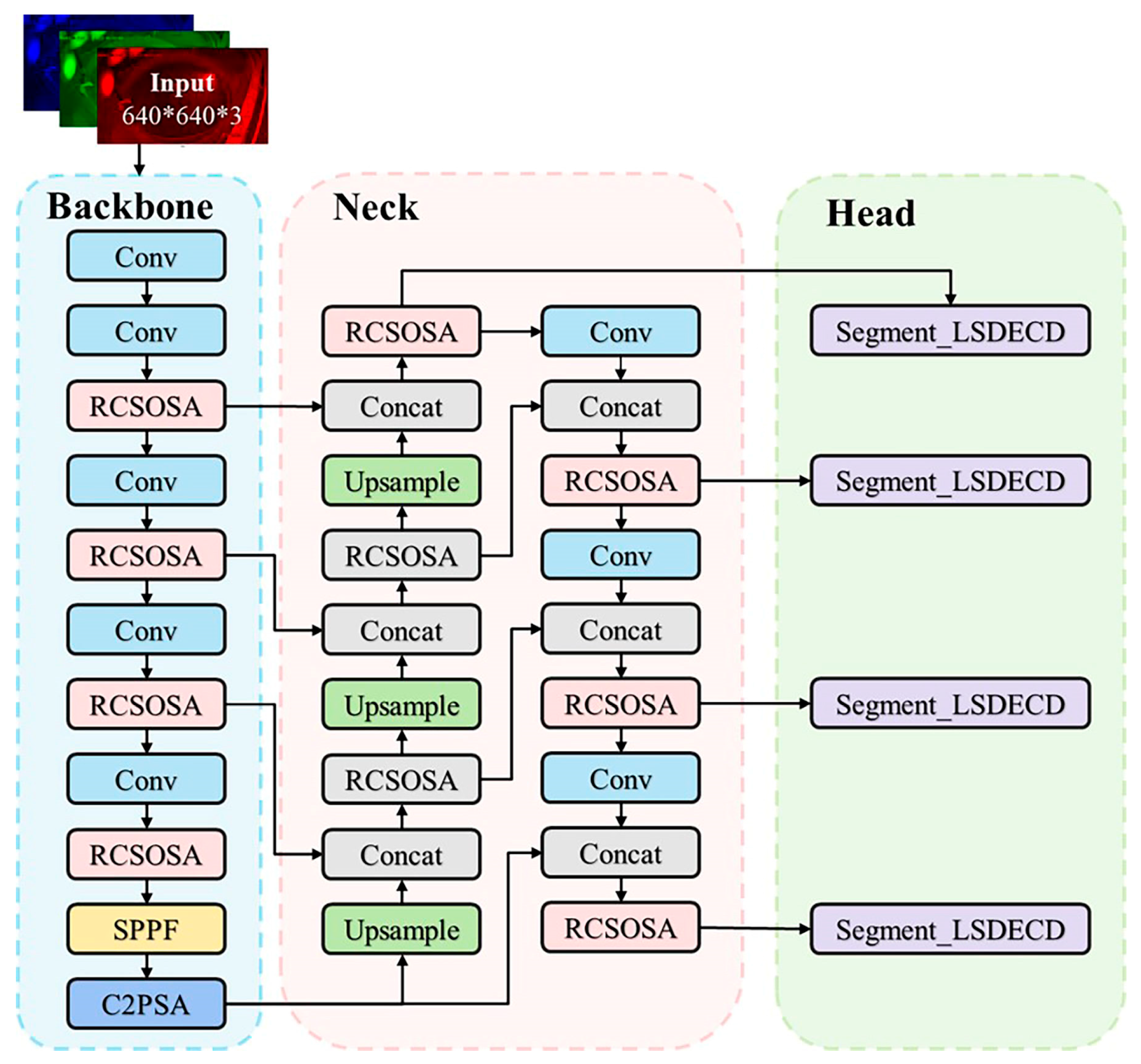
In this study, “lightweight” refers to the optimization of the network architecture to reduce computational and storage overhead while maintaining high accuracy. FishSegNet-PRL achieves efficient small-object detection and boundary refinement through innovative designs such as the introduction of the P2 detection layer, RCSOSA module, and LSDECD, enabling the model to operate in real-time within resource-constrained aquaculture environments. First, considering that fish schools often rapidly aggregate and disperse within short periods during feeding, small targets and local edges are frequently difficult to segment clearly. To address this, a P2 layer was introduced into the detection head, enabling predictions on higher-resolution feature maps. This enhances the detection of small targets and edge details, thereby providing more reliable segmentation results for subsequent calculations such as pixel area and nearest-neighbor distance [30]. The P2 detection layer enhances the ability to detect small objects, particularly in situations where fish schools are aggregated, reducing the missed detection issues caused by targets being too small. However, simply adding a detection layer is not sufficient to handle the challenges of overlap and occlusion in complex aquaculture backgrounds. Therefore, RCSOSA (Reparameterized Convolution with Channel-Shuffle and One-Shot Aggregation) modules were extensively integrated into both the backbone and the head. During training, multi-branch structures were adopted to enhance feature representation, while during inference, structural re-parameterization consolidated the branches into a single path. This design strengthened cross-scale information flow and edge feature extraction without increasing inference cost [31]. The RCSOSA module reduces computational and storage costs, improving the model’s performance in complex backgrounds without sacrificing accuracy. Finally, in the segmentation head, we designed the LSDECD (Lightweight Spatial-Dense Enhanced Context Decoder). This decoder extracts multi-directional texture and edge information using DEConv layers with shared weights, while group normalization (GN) and learnable dynamic scale factors are applied to improve the fitting capacity for multi-scale fish bodies. The LSDECD reduces the model’s computational burden through a lightweight design, while preserving boundary details. With these improvements, the proposed FishSegNet-PRL model achieves higher instance segmentation accuracy and real-time performance compared to the baseline YOLOv11-seg. It enables more precise fish body segmentation under complex aquatic backgrounds and provides a solid foundation for objective feeding intensity quantification. Experimental results demonstrate substantial improvements in both mAP50 and mAP50–95, along with high deployment efficiency, offering strong support for intelligent feeding management and health monitoring in aquaculture. The improved model is illustrated in Figure 5.

2.2.2. RCSOSA Module

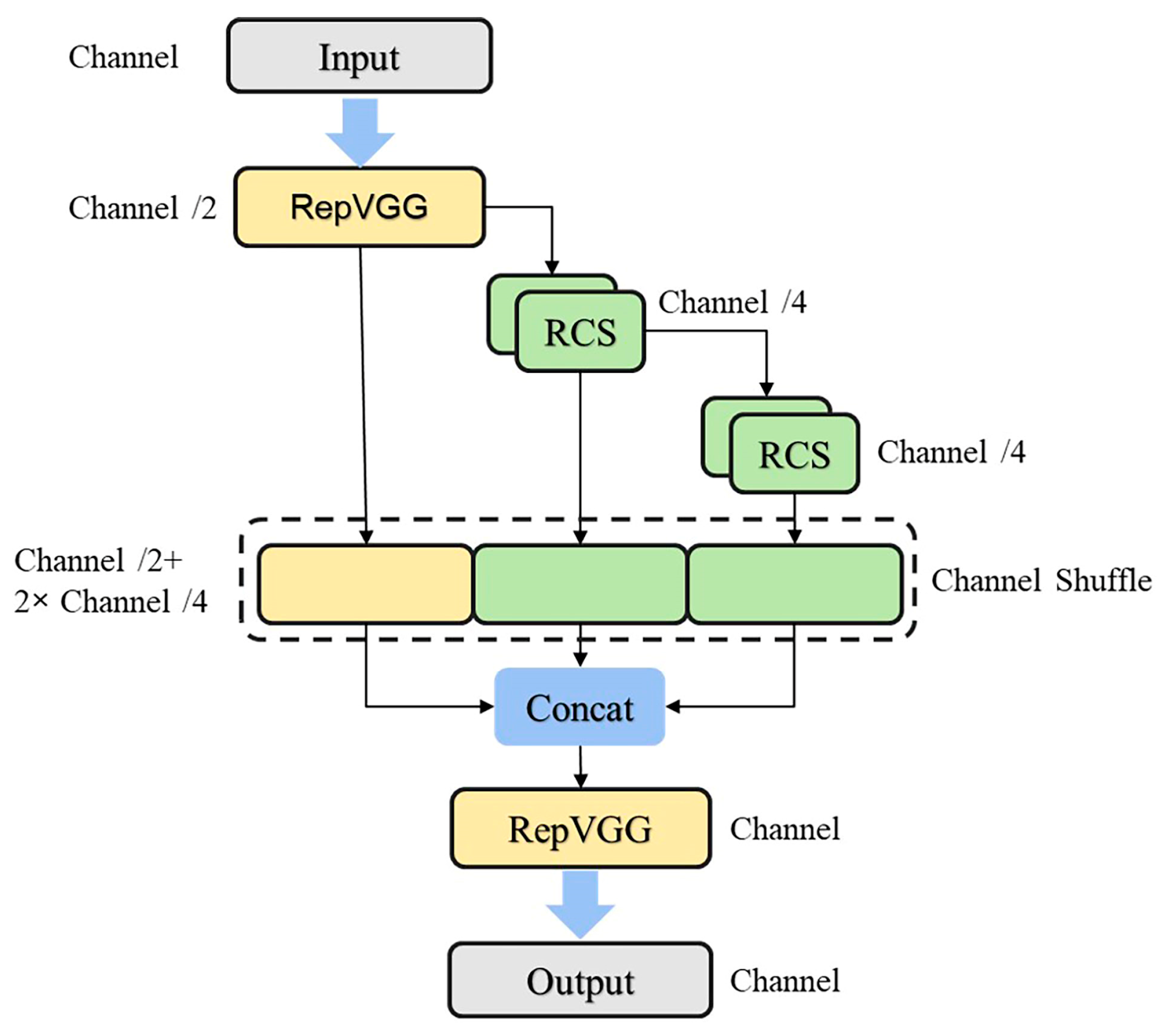
RCSOSA (Reparameterized Convolution with Channel-Shuffle and One-Shot Aggregation) is an efficient module designed for object detection and instance segmentation, aimed at significantly reducing computational and storage costs without sacrificing accuracy. Compared with the conventional C3k2 module, RCSOSA integrates channel-shuffle and reparameterized convolution (RCS) techniques, while introducing a one-shot aggregation (OSA) strategy to achieve efficient unification between the training and inference stages. During training, RCSOSA employs a multi-branch structure to obtain richer and more diverse feature representations; through the reparameterization mechanism, the inference process can substantially reduce computational overhead while maintaining accuracy.
Specifically, RCSOSA establishes an efficient information exchange mechanism among feature channels through channel-shuffle operations, enabling deep networks to achieve cross-channel feature interaction at relatively low computational cost. Reparameterized convolution simplifies complex multi-branch structures into an equivalent single convolution branch during inference, ensuring diverse feature representations in the training stage while improving inference efficiency. The OSA strategy integrates multi-level representations with a “one-shot aggregation, less redundancy” approach, facilitating efficient fusion of features across different levels and enhancing the model’s semantic information extraction capability. In terms of structural design, RCSOSA stacks RCS modules to achieve feature cascading, strengthening information flow between adjacent layers. Multi-scale feature fusion is further realized through upsampling and downsampling operations, which promote information exchange across different prediction layers. The architecture of the RCSOSA module is illustrated in Figure 6 [32].
In the task of quantifying feeding intensity of mandarin fish, fish schools often exhibit high-density aggregation and rapid movements within complex and dynamic underwater backgrounds. Under such conditions, single convolutional features struggle to clearly delineate individual boundaries during local collisions and occlusions. Moreover, insufficient modeling of inter-channel correlations and global context leads to the loss of fish edge information or its suppression by interfering background features. The RCSOSA module enhances cross-layer and cross-channel information exchange, thereby preserving fish body edges and fine details as much as possible while suppressing irrelevant interference in complex scenarios. Channel attention is employed to emphasize features related to morphological details such as fish body shape and fin rays, while spatial attention highlights local edge contours, improving segmentation accuracy and boundary clarity. In addition, the residual structure alleviates gradient vanishing in deep training, reducing the likelihood of missing small targets or fine edges. Experimental results demonstrate that incorporating RCSOSA significantly improves model performance on both mAP50 and mAP50–95 metrics, with particularly notable gains in small-object detection and edge segmentation accuracy. Furthermore, owing to its structured re-parameterization design, computational efficiency during inference is greatly enhanced, effectively meeting the dual requirements of speed and accuracy for real-time monitoring.

2.2.3. P2 Detection Head

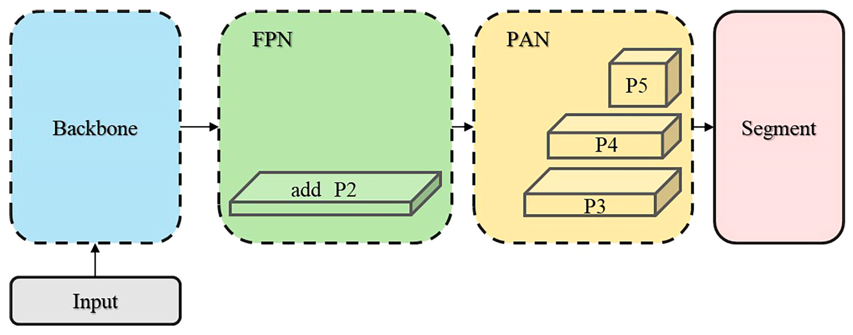
The P2 detection head is specifically optimized for small-object scenarios, with the core objective of significantly enhancing the model’s ability to perceive and represent fine-grained targets. Traditional detection heads mainly rely on multi-scale features from P3–P5 for prediction, which are suitable for medium and large objects but often lead to missed detections or imprecise edge segmentation for small targets (e.g., juvenile fish in schools or local postural features of mandarin fish during feeding). As shown in Figure 7, the P2 detection layer is constructed on shallow feature maps, allowing it to retain more fine-grained spatial information and texture features [33]. Compared with traditional detection layers, the P2 layer offers higher resolution, making it better suited for segmenting and detecting smaller individual targets.
In the application scenario of mandarin fish feeding intensity quantification, fish schools typically exhibit a dynamic pattern of “rapid aggregation–swift dispersion” during feeding, with individuals in close proximity and frequent postural changes. With the introduction of the P2 layer, the model can perform finer representation and segmentation on higher-resolution feature maps for small-sized fish bodies, localized biting actions, and neighboring relationships between individuals. This not only improves the accuracy of instance segmentation but also provides reliable data support for subsequent pixel area calculations (to measure fish body coverage) and nearest-neighbor distance metrics (to reflect local crowding levels within the school).
With the addition of the P2 detection layer, the model’s robustness under complex backgrounds was enhanced, and the recall rate for small targets was significantly improved. Experimental results indicate that incorporating the P2 detection layer leads to substantial improvements in mAP50–95, while enabling more accurate characterization of fish school spatial distribution and activity levels during the calculation of feeding intensity metrics. In summary, the introduction of the P2 detection layer not only optimizes the model’s detection performance but also provides a solid technical foundation for the fine-grained quantification of mandarin fish feeding behavior.

2.2.4. LSDECD

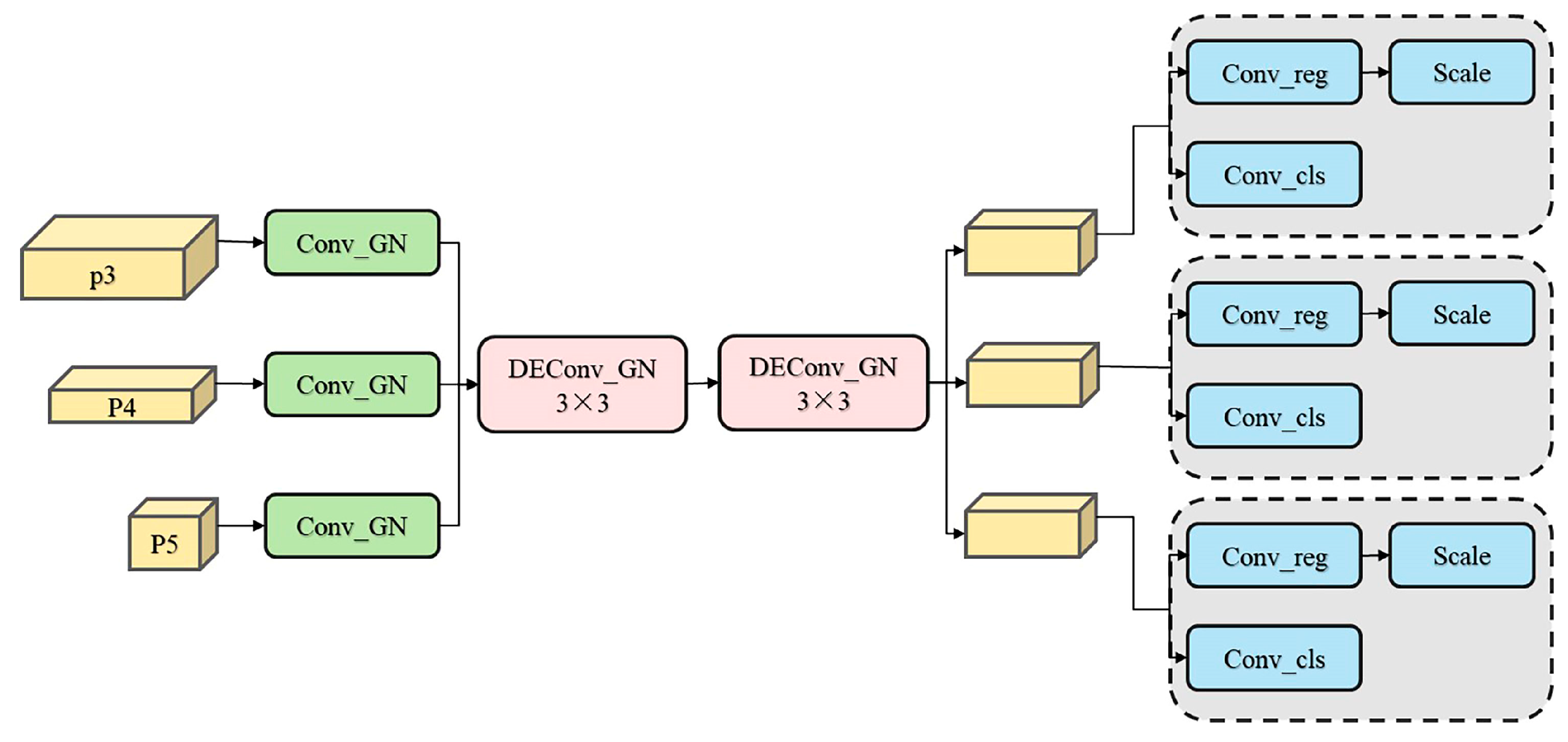
Within the YOLOv11 framework, the traditional segmentation detection head continues the decoupled design of YOLOv8, where classification and localization are performed independently through multiple convolutional layers. Although this strategy can improve accuracy, it incurs a relatively high computational cost in resource-constrained environments and lacks sufficient information exchange among detection heads at different scales, thereby limiting precise segmentation of small targets in complex backgrounds. To address these issues, we propose the LSDECD (Lightweight Spatial-Dense Enhanced Context Decoder) segmentation head. The core idea is to introduce detail-enhancement convolution (DEConv) and a shared-weight mechanism, which significantly reduce computational complexity while maintaining accuracy.
The structure of LSDECD is illustrated in Figure 8 [34]. It receives feature maps at three scales (P3, P4, P5) from the neck, and first applies a 1 × 1 convolution with group normalization (GN) to adjust the number of channels, stabilize feature distribution, and align the representational space of the classification and localization branches. Subsequently, each branch passes through two 3 × 3 DEConv modules with shared parameters, which expand the receptive field and integrate multi-scale contextual information. The DEConv module consists of five parallel convolutional layers: standard convolution (Conv), central difference convolution (CDC), angular difference convolution (ADC), horizontal difference convolution (HDC), and vertical difference convolution (VDC). Among these, the difference convolution layers focus on capturing edge and texture variations along different directions, while the standard convolution is responsible for extracting pixel intensity features. By fusing the outputs of these parallel convolutions, DEConv generates more detailed and information-rich feature maps, thereby providing more reliable fine-grained support for subsequent boundary prediction and instance segmentation.
At the end of each branch, LSDECD applies a 1 × 1 convolution to decouple the computation of classification loss (ClsLoss, BCE) and regression loss (BBoxLoss, CIoU + DFL). In addition, a Scale layer is introduced in the regression branch, adding a learnable dynamic factor to each detection head in order to adapt to variations in target scales during training. This design enables the model to dynamically adjust the size of predicted bounding boxes based on gradient feedback, which is particularly effective for small-object segmentation.
In the application scenario of mandarin fish feeding intensity quantification, LSDECD can more effectively capture edge and texture details of fish bodies, reducing missed segmentations of small targets and overlapping individuals. This provides more accurate segmentation results for subsequent pixel area calculations and nearest-neighbor distance measurements. Experimental results show that introducing the LSDECD segmentation head leads to significant improvements in both mAP50–95 and mIoU, while maintaining fewer parameters and lower inference latency than conventional detection heads. These results demonstrate the advantages of LSDECD in terms of both accuracy and efficiency.

2.3. Feature Construction for Feeding-Intensity

To achieve comparable and robust thresholds across different aquaculture tanks, resolutions, and frame rates, we adopted the dimensionless approach from Table 2 for data processing. In this process, we first denote the foreground union obtained from the instance segmentation as A u n i o n , and normalize the area according to the Region of Interest (ROI). Simultaneously, the distance is normalized based on the scene scale R (such as the tank radius), and time is normalized according to the frame interval. Through these steps, we derived the five intensity metrics from Table 2: total area, nearest neighbor distance, area growth rate, cluster count, and perimeter-to-area ratio.
Specifically, under the condition of fixed fish school size, an increase in total area typically reflects a more dispersed fish distribution or the expansion of the hotspot coverage area, which is usually associated with a decrease in feeding intensity. On the other hand, a reduction in the mean nearest neighbor distance indicates increased crowding and intensified competition between individuals, which negatively correlates with feeding intensity. Conversely, when the area growth rate exhibits a sharp positive spike, it usually corresponds to the short-term aggregation or rapid upward movement of the fish, indicating a feeding burst period with a significant increase in feeding intensity. During the feeding burst phase, the number of clusters typically decreases from multiple fragmented small clusters to fewer but more concentrated and active clusters, which positively correlates with feeding intensity. Finally, an increase in the perimeter-to-area ratio reflects a rougher fish school boundary and frequent deformations (edge “tearing” or enhanced mobility), which generally correlates positively with feeding intensity.
To eliminate pseudo-instances with small areas and extreme aspect ratios, we performed relevant filtering within fixed or adaptive ROIs. After each instance mask was restored to the original resolution using nearest-neighbor interpolation, we calculated the union of the foreground and computed the perimeter-to-area ratio using the outer contour length. Next, we constructed a distance matrix for each instance’s centroid and calculated the nearest neighbor distance by taking the minimum distance. Additionally, since frame-by-frame signals are often significantly affected by aeration and reflections, we grouped the data into blocks of g frames, calculated the mean and median, and used LOESS and LOWESS methods for smoothing to preserve phase transitions while suppressing high-frequency noise. LOESS is a robust local regression method suitable for noisy time series and effectively extracts smooth trends. Based on the five indicators mentioned above, we jointly describe the “dispersion” and “activity” of the fish school to characterize the feeding process. We then compared these with manually and sensor-annotated start—active—decline—stop intervals. To assess the consistency across different phases, we used temporal Intersection over Union (IoU) for evaluation. Empirically, the active phase typically shows a decrease in total area and an increase in nearest neighbor distance (with rougher boundaries and stronger local disturbances), while the decline and stop phases show the opposite trend. This “spacing—crowding—shape” interplay aligns with observations of neighbor structure and boundary disturbances in group behavior, further validating our method.
Through this comprehensive analysis of temporal and spatial features, we are able to stably and repeatably describe and score the feeding intensity of fish schools, providing reliable technical support for intelligent aquaculture systems.

2.4. Feeding-Intensity Modeling with LightGBM

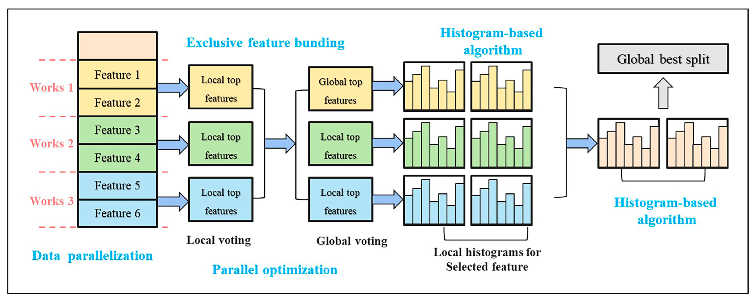
In this study, LightGBM was employed to perform regression modeling on the five categories of group-level features described in Section 2.3, generating frame/group-level feeding intensity curves and stage boundaries. LightGBM is a histogram-based GBDT that grows leaf-wise (best-first) to maximize loss reduction. It further leverages GOSS (Gradient-based One-Side Sampling) and EFB (Exclusive Feature Bundling) to exploit gradient and sparsity priors for efficient training, achieving a balance between accuracy and speed. This makes it well suited for small- to medium-sized datasets and online deployment scenarios. Compared to other regression models (such as XGBoost and Random Forest), LightGBM demonstrates higher efficiency and better performance when handling large-scale data and high-dimensional features, making it more suitable for the data characteristics of this experiment [35,36]. The principle of LightGBM is illustrated in Figure 9 [37].
In mandarin fish feeding intensity quantification, the group-level indices extracted by FishSegNet-PRL can be used as feature inputs to LightGBM. Leveraging the tree model’s capacity to capture nonlinear relationships and threshold effects, LightGBM can learn the integrated mapping of feeding intensity under small-sample and heterogeneous-feature conditions, while also providing feature importance to support interpretable analysis and feeding control. Combined with cross-validation and evaluation metrics such as MAE and temporal-domain IoU, the fitted intensity curves and event boundaries can be robustly assessed, forming a stable and reproducible framework for feeding intensity evaluation.

2.5. Evaluation Metrics

2.5.1. Evaluation Metrics for FishSegNet-PRL

In evaluating model performance, this study employed multiple metrics, including Precision (P), Recall (R), Precision–Recall (P–R) curve, F1 curve, Intersection over Union (IoU), mean Intersection over Union (mIoU), and Frames Per Second (FPS), to comprehensively assess the effectiveness of the object detection and instance segmentation model.
Precision (P) and Recall (R)
Precision (P) measures the proportion of correctly predicted positive samples among all samples predicted as positive; Recall (R) measures the proportion of actual positive samples that are correctly identified by the model among all positive samples. Their values range from 0 to 1, and the formulas are as follows:
P = X T P X T P + X F P
R = X T P X T P + X F N
In Formulas (1) and (2) above, Precision measures the proportion of correctly predicted positive samples among all samples predicted as positive, reflecting the accuracy of the model. Recall measures “how many of all true positive samples are successfully identified by the model,” emphasizing the model’s detection capability and sensitivity. Here, X T P denotes the number of correctly identified mandarin fish instances, X F P denotes the number of false positives incorrectly recognized as mandarin fish, and X F N represents the number of false negatives where mandarin fish were mistakenly classified as other objects. All quantities are expressed as counts.
P–R Curve and mAP
The P–R curve provides an intuitive visualization of the relationship between precision and recall across the dataset. The area enclosed by the curve and the coordinate axes corresponds to the mean Average Precision at 0.5 IoU (mAP50). A higher mAP50 indicates stronger capability of the model in predicting object locations, whereas a higher mAP50–95 suggests more robust overall accuracy across different application scenarios and requirements. Both metrics range between 0 and 1 and serve as important evaluation indicators in this study. The formulas are as follows:
m A P & @ 50 = 1 m 0 1 P R d R
m A P @ 50 95 = 1 10 j = 1 10 0 1 P ( R ) d R
Intersection over Union (IoU) and mIoU
IoU measures the degree of overlap between the predicted result and the ground-truth annotation. The mean IoU (mIoU) is obtained by averaging IoU across all categories. The corresponding formulas are as follows:
I o U i = T P i T P i + F P i + F N i
m I o U = 1 N i = 1 N I o U i
In Formulas (5) and (6), T P i denotes the number of pixels in class i that are predicted as positive and are truly positive; F P i denotes the number of pixels in class i that are predicted as positive but are actually negative; F N i denotes the number of pixels in class i that are truly positive but predicted as negative; and N is the total number of classes. mIoU measures the average overlap between model predictions and ground-truth annotations, with values ranging from 0 to 1 [38]. A larger value indicates that the segmentation results are closer to the ground truth. mIoU reflects the segmentation accuracy of the FishSegNet-PRL model for both mandarin fish and background regions. A higher mIoU implies greater accuracy in delineating fish body edges and overall contours, thereby providing more reliable data for subsequent pixel area calculations and nearest-neighbor distance measurements.
Frames per Second (FPS)
Frames per second (FPS) measures the inference speed of the model, expressed in frames per second. It indicates the number of image frames that can be processed each second under specific hardware conditions, input resolution, and batch size, and is used to evaluate the model’s real-time performance and deployment efficiency in practical applications. Comparative experiments should also specify the testing environment and parameter configurations to ensure reproducibility of results.

2.5.2. Evaluation Metrics for the LightGBM Model

To evaluate the performance of the LightGBM model, frame-level regression error (Mean Absolute Error, MAE) and Intersection over Union (IoU) were employed to assess the effectiveness of the feeding intensity quantification model.
The formulas for calculating MAE and IoU are as follows:
MAE = 1 T t = 1 T FI t ^ F I t
R M S E = 1 T t = 1 T F t ^ F t 2
R 2 = 1 t = 1 T F t F ^ t 2 t = 1 T F t F ¯ 2
In Formulas (7)–(9), MAE measures the numerical error of the intensity curve and reflects the goodness of fit of the model. R2 indicates the explanatory power of the predicted values with respect to the ground truth. RMSE represents the “average deviation” between predicted and true values. FI t ^ denotes the predicted feeding intensity, F I t denotes the ground-truth intensity, and T represents the number of evaluation frames.

2.5.3. Quantification of Fish School Features and Feeding Intensity Indicators

In order to evaluate the temporal overlap between the manually annotated feeding periods and the model-predicted feeding periods, we define the following formula:
I o U time = L int t e t s + t ^ e t ^ s L int 0,1 ,   L int = max 0 , min t e , t ^ e max t s , t ^ s
In Formula (10), IoU time measures the temporal overlap between the predicted interval and the annotated interval. t s , t e denotes the manually annotated feeding period, t s , t ^ s denotes the model-predicted period, and L int represents the length of the overlapping duration between the two intervals.

3. Results

3.1. Experimental Environment

The experiments were conducted on a Windows 10 Professional (10.0.19045, 64-bit) operating system using Python 3.12.11 and the PyTorch 2.7.1+cu128 deep learning framework. The hardware configuration included an Intel Core i9-11900K CPU, CUDA runtime version 11.2.67, and an NVIDIA RTX A5000 GPU. Key hyperparameters for model training were set as follows: initial learning rate = 0.01, batch size = 8, number of iterations = 400, and optimizer = SGD algorithm.

3.2. Instance Segmentation on PRLSFISH

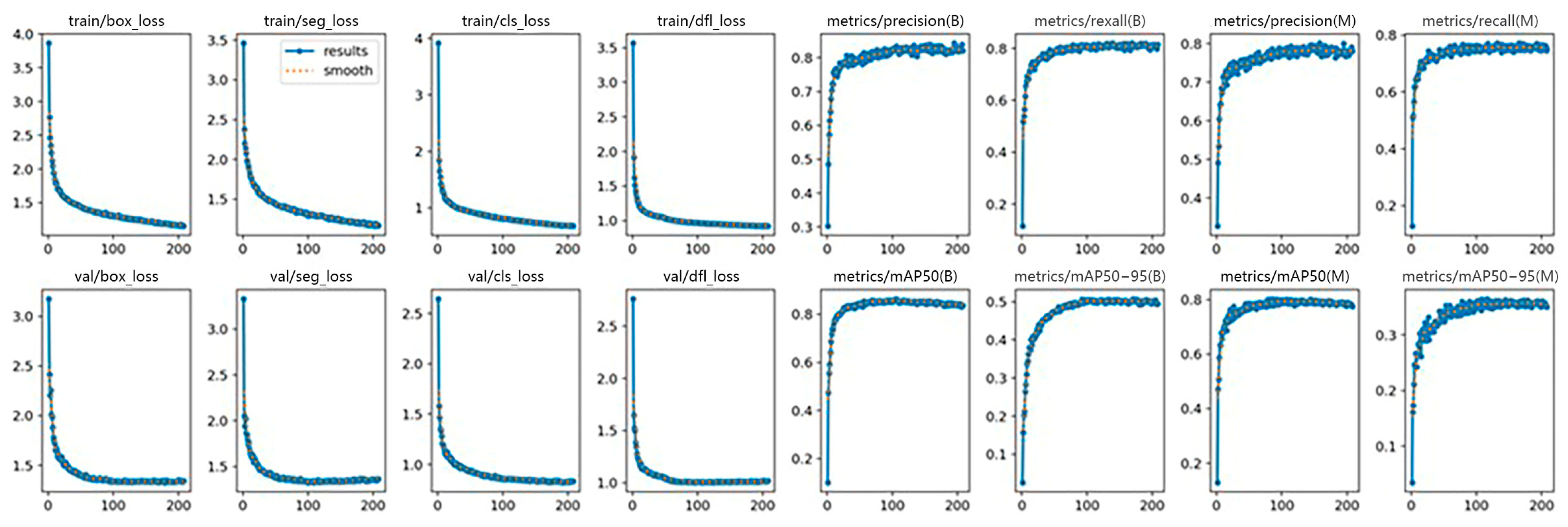
For mandarin fish, the FishSegNet-PRL model achieved a box precision of 97.8%, a recall of 82.8%, and an mAP50 of 80.1%. For masks, the precision reached 78.5%, the recall 74.7%, and the mAP50 79.4%. The results of the FishSegNet-PRL model on the dataset are illustrated in Figure 10.

3.3. Ablation Study

To evaluate the contribution of each improved module, ablation experiments were conducted using YOLOv11-seg as the baseline model, focusing on the P2 detection layer, RCSOSA module, and LSDECD module. Under identical dataset, input size, and training strategy conditions (Learning rate = 0.01, batch size = 8, image size = 640, number of training epochs = 400), only the presence or absence of these three modules was varied to form eight configurations (N1–N8): YOLOv11-seg (N1), YOLOv11-seg + P2 (N2), YOLOv11-seg + RCSOSA (N3), YOLOv11-seg + LSDECD (N4), YOLOv11-seg + P2 + RCSOSA (N5), YOLOv11-seg + P2 + LSDECD (N6), YOLOv11-seg + RCSOSA + LSDECD (N7), and YOLOv11-seg + P2 + RCSOSA + LSDECD (N8). Evaluation metrics included box-level Precision (P), Recall (R), mAP50, and mAP50–95, as well as mask-level Precision (P), Recall (R), mAP50, and mAP50–95. Frames per second (FPS) were also recorded to assess real-time performance (see Table 3).
The results show that introducing the P2 layer alone yielded the most notable improvements in recall for small targets and boundary regions. RCSOSA provided certain feature enhancement when used independently, but the accuracy gains were limited and occasionally accompanied by minor fluctuations. LSDECD contributed more stable improvements in boundary refinement and overall accuracy. The combination of multiple components achieved generally superior performance, with the P2 and LSDECD modules being particularly effective in boosting accuracy. Taking the PRLSFISH dataset as an example, the lightweight design significantly improved the detection of small targets and boundary segmentation, with FishSegNet-PRL (N8) outperforming the original YOLOv11-seg (N1) model, achieving increases of 4.6% and 13.2% in Box mAP50 and Mask mAP50, respectively. Moreover, despite a slight decrease in FPS, this design still maintains efficient real-time inference performance, demonstrating that the lightweight design effectively controls computational overhead while improving accuracy.

3.4. Comparative Study

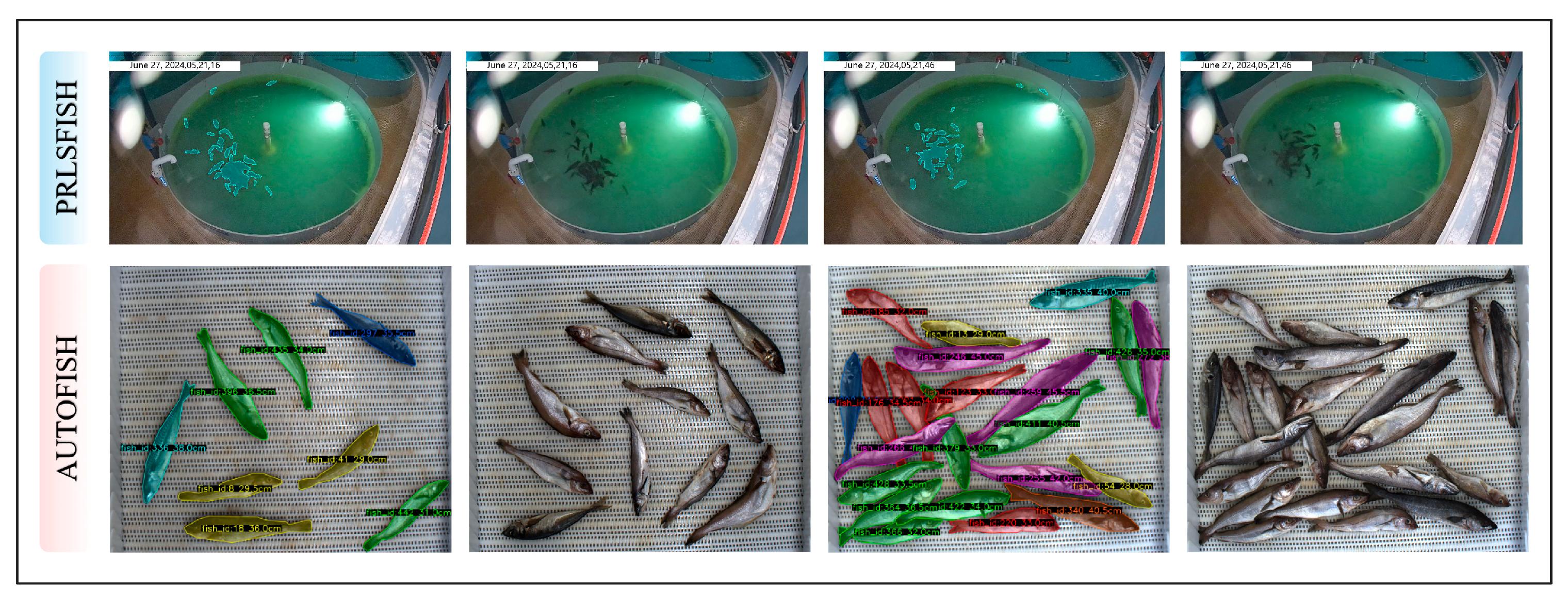
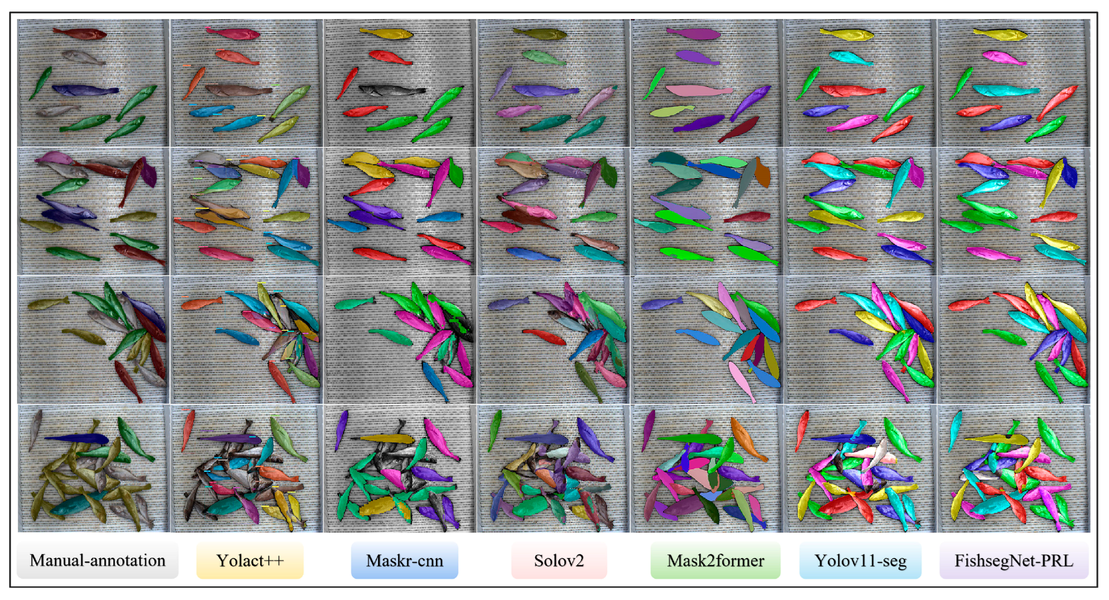
At present, there is a lack of publicly available instance segmentation datasets tailored to factory-scale fish farming scenarios, making it difficult to conduct cross-model comparisons under unified annotations and reproducible experimental conditions. The proposed FishSegNet-PRL is designed for practical aquaculture operations and specifically optimized for challenges such as small targets, high-density overlap, strong reflections, green-biased illumination, turbidity, and motion blur (e.g., by introducing a small-object detection layer, boundary-refinement decoder, and cross-layer contextual enhancement). To objectively verify the effectiveness and generalizability of these improvements, after training and evaluation on our self-constructed PRLSFISH dataset, we further selected the most task-relevant and well-annotated public dataset, AutoFish (1500 images covering 454 fish, with instance segmentation masks, individual IDs, and length annotations), for additional comparative experiments. A comparison of datasets is provided in Figure 11. We compared five models: Mask R-CNN, Mask2Former, YOLACT++, SOLOv2, and YOLOv11-seg, ensuring consistency in both training and inference processes. All models used a 0.5 confidence threshold to convert the output probability maps into binary masks, ensuring that only predictions with confidence higher than this threshold were considered valid. This threshold choice balances false positives and false negatives, ensuring the accuracy and recall of the segmentation results. We selected segmentation results for four levels of fish school stacking from the public dataset AutoFish for comparison, with results from the mainstream models shown in Figure 12. These comparison results are more closely aligned with the data from our custom dataset PRLSFISH, particularly the fish school stacking variations in Chinese perch under different feeding intensities.
The experimental results show that FishSegNet-PRL achieved an mAP50 of 98.2%, YOLOv11-seg achieved an mAP50 of 97.6%, Mask R-CNN (ResNet50) achieved an mAP50 of 92.4%, Mask2Former achieved an mAP50 of 94.6%, YOLACT++ achieved an mAP50 of 91.5%, and SOLOv2 achieved an mAP50 of 93.2%. In the scenario with large targets and relatively low stacking (AutoFish), the overall accuracy of all methods was similar. However, as the stacking degree increased, our model FishSegNet-PRL showed a slight improvement over the baseline YOLOv11-seg, achieving better segmentation of individual fish with fewer missed detections. This is particularly aligned with the severe fish school stacking observed in Chinese perch under different feeding intensities. In contrast, in complex underwater aquaculture scenarios (PRLSFISH), where the high proportion of small targets, severe occlusions/overlaps, and imaging degradation are prevalent, YOLOv11-seg showed a more pronounced drop in accuracy. Benefiting from task-specific optimizations tailored for small-object detection and aquaculture conditions, FishSegNet-PRL achieved significantly better performance in this challenging environment. In summary, our method can be regarded as a specialized domain-adaptive model: it delivers substantial gains in real farming environments, while in simpler scenarios it maintains comparable or slightly better accuracy than mainstream approaches with higher efficiency. This validates the effectiveness and transferability of the proposed improvements in the target application. The observed cross-domain differences essentially stem from a degradation pathway of physical degradation → feature degradation → task degradation: underwater absorption, scattering, and backscattering cause reduced contrast, hazing, and color bias; bubbles and particulates generate pseudo-foreground artifacts; combined with small targets, occlusions, and low contrast, these factors make generic models more prone to missed and false detections. To address this pathway, our approach leverages the P2 detection head to preserve high-resolution details, the RCSOSA attention mechanism to suppress scattering noise while highlighting boundary cues, and the lightweight LSDECD to stabilize mask details—achieving a superior balance between accuracy and speed in complex domains.

3.5. Feeding-Feature Dynamics & Phase Consistency

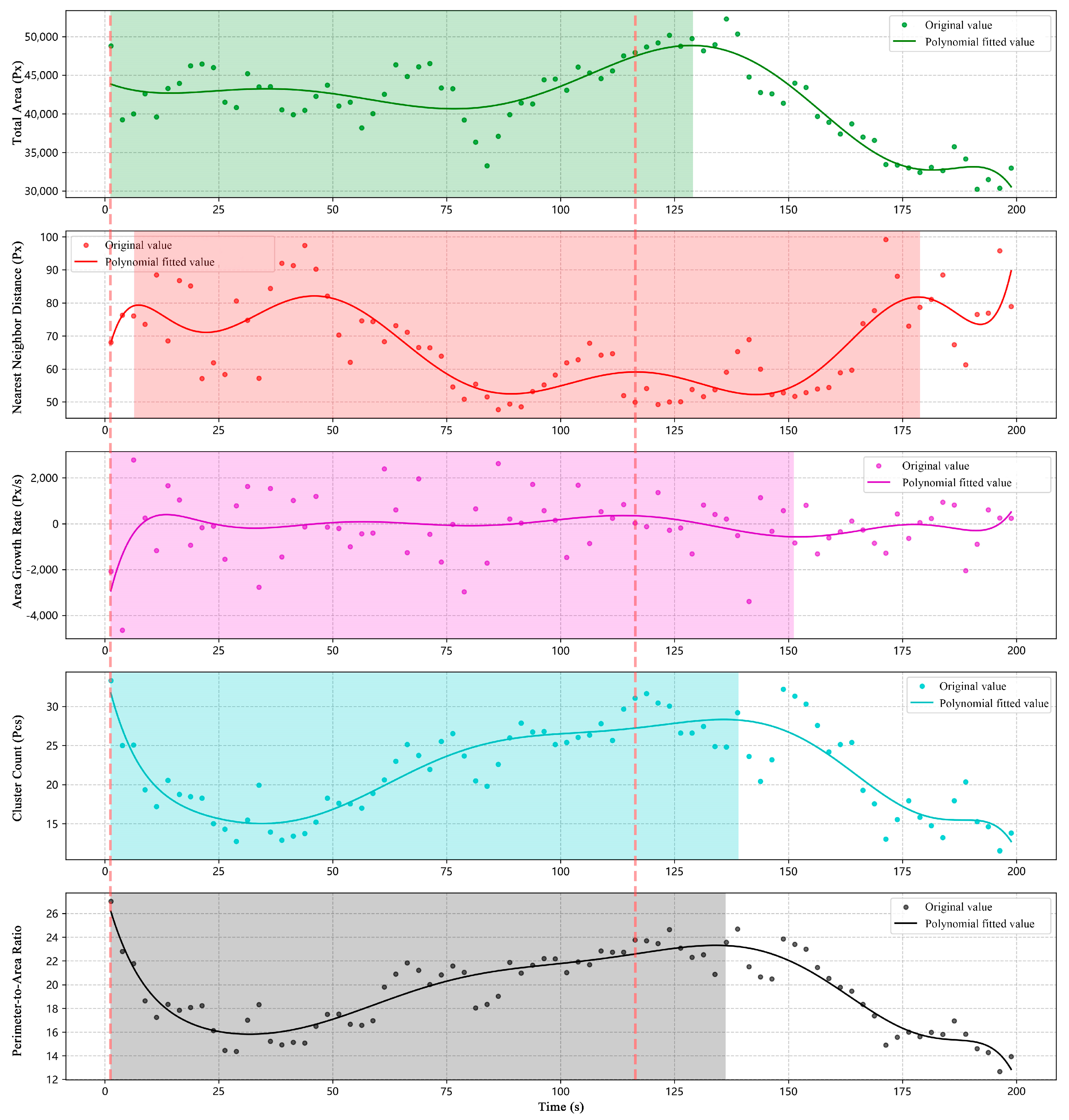
Figure 13 presents the time series and polynomial-smoothed curves of five group-level features computed from instance segmentation results: total area of the fish school, nearest-neighbor distance, area growth rate, cluster number, and perimeter-to-area ratio. Total area, nearest-neighbor distance, and cluster number collectively characterize dispersion, while area growth rate and perimeter-to-area ratio reflect activity. In the figure, vertical dashed lines indicate the ground-truth feeding intervals, and shaded backgrounds denote the predicted feeding intervals, providing an intuitive comparison of feature variations across different stages and thereby assessing their representational capacity for feeding intensity.
As shown in Figure 13, dispersion-related features (cluster number, total school area, and nearest-neighbor distance) exhibit a significant negative correlation with feeding intensity. During strong feeding phases, these three features are overall lower and fluctuate less than in moderate phases, reflecting rapid aggregation of the fish school; in non-feeding phases, they are generally higher than in weak feeding, indicating a more dispersed distribution. Activity-related features (area growth rate and perimeter-to-area ratio) display a positive correlation with feeding intensity. In strong feeding phases, their fluctuations are markedly greater than in moderate phases, indicating intense competition for feed; in non-feeding phases, they are substantially lower than in weak feeding, suggesting reduced activity. Although short-term fluctuations exist due to schooling effects and individual differences, the overall trends remain stable and gradually converge toward the end of feeding. Quantitative evaluation shows that the IoU values for total area, nearest-neighbor distance, area growth rate, cluster number, and perimeter-to-area ratio are 90.6%, 60.8%, 77.4%, 84.2%, and 87.3%, respectively, with an overall mIoU of 80.1%. These results indicate that the selected features can effectively capture the stage-wise variations in feeding intensity.

3.6. Feature Importance & Elimination

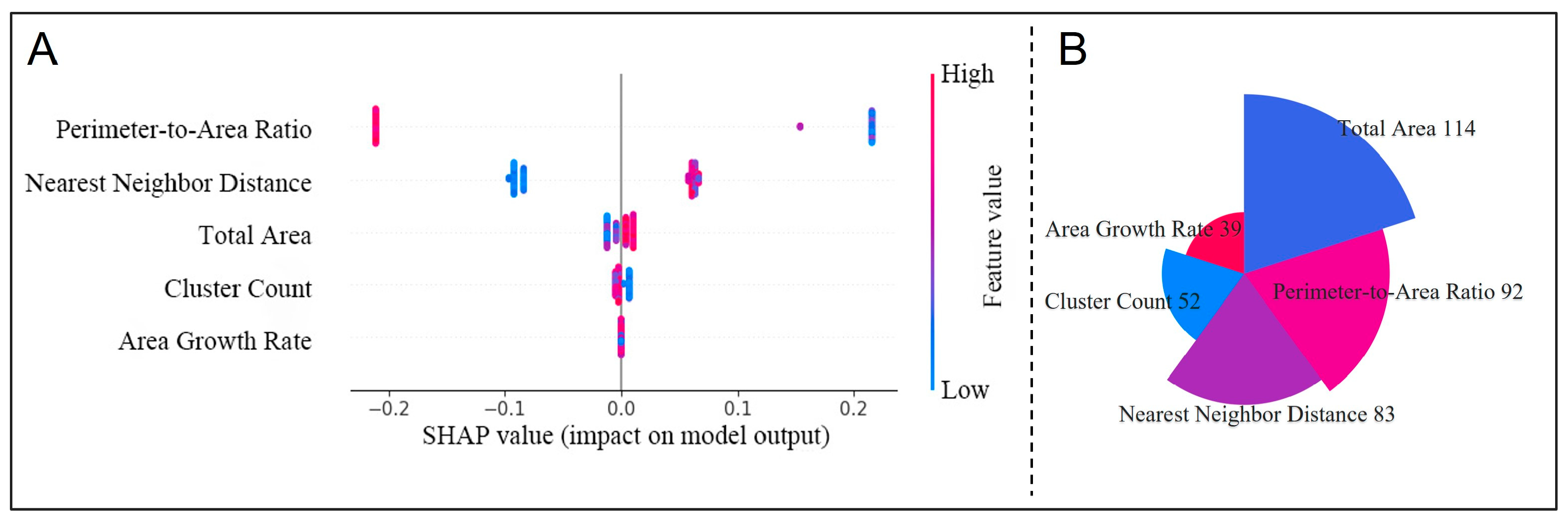
To interpret the basis on which the model discriminates feeding intensity and to identify the most effective group-level features, LightGBM was employed as the regressor for importance evaluation and interpretability analysis of the five input features (total area, nearest-neighbor distance, area growth rate, cluster number, and perimeter-to-area ratio). In the model training process, we selected the following LightGBM hyperparameters: learning rate (learning_rate = 0.05), number of leaves (num_leaves = 50), number of trees (n_estimators = 100), and random seed (random_state = 42). Figure 14A presents the SHAP beeswarm plot (with the horizontal axis indicating feature impact on model output, and colors representing high and low feature values, allowing simultaneous observation of both contribution direction and magnitude). Figure 14B shows the feature-importance rose chart, summarizing each feature’s overall contribution to the predictions. Furthermore, using a “full features–stepwise reduction” approach, we performed backward elimination to examine the impact of different feature combinations on model performance (RMSE, MAE, and R2), thereby achieving an optimal balance between predictive performance and model simplicity.
As shown in Figure 14, total area contributed the most to the model, followed by perimeter-to-area ratio and nearest-neighbor distance, while cluster number ranked in the middle and area growth rate contributed the least. The beeswarm plot further indicates that nearest-neighbor distance is generally negatively correlated with feeding intensity, whereas perimeter-to-area ratio is predominantly positively correlated, consistent with the earlier analysis of dispersion and activity features. Back-ward elimination experiments revealed that removing “area growth rate” and “cluster number” improved model performance, with RMSE decreasing by 0.0922, MAE decreasing by 0.0879, and R2 increasing by 0.1771. However, further removal of “nearest-neighbor distance” degraded performance, indicating that this feature is essential for maintaining overall fitting ability. Integrating the SHAP ranking with the backward elimination results, the recommended optimal simplified feature set comprises total area + nearest-neighbor distance + perimeter-to-area ratio. This combination substantially simplifies the model while preserving predictive accuracy and improving generalizability, thereby providing a more robust and interpretable input design for subsequent feeding-intensity modeling and deployment.

3.7. Feeding-Intensity Curve & Stage Detection

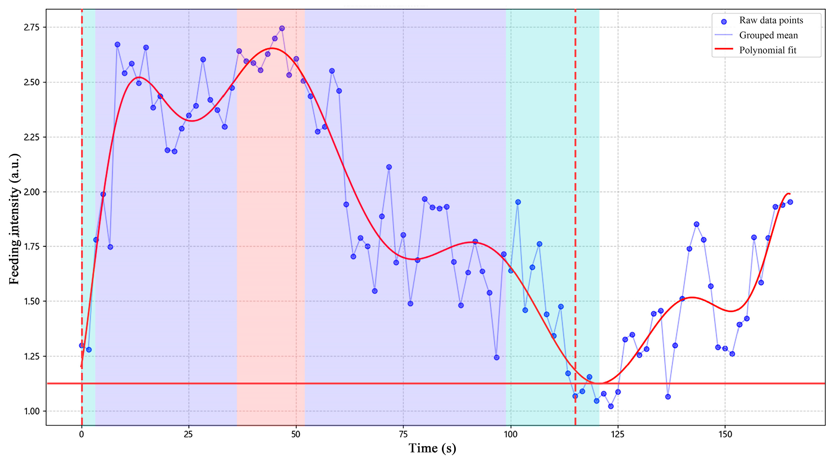
In animal behavior research, feeding intensity is an important indicator for assessing feeding motivation and behavioral rhythms. Figure 15 illustrates the temporal variation in fish-school feeding intensity along with polynomial fitting results, with the overall process divided into four phases. During the initiation phase, feeding intensity rapidly increased following feed delivery and reached a local peak at approximately 16 s. In the active phase, the global maximum occurred at around 45 s, reflecting the most concentrated and vigorous feeding behavior. In the decline phase, intensity gradually decreased and stabilized at a moderate level, representing differences in satiety among individuals and adaptive adjustments. In the termination/transition phase, feeding intensity dropped sharply and frequently fell below the threshold, indicating that the fish school had largely ceased feeding. The slight rebound observed in the final segment was likely due to group swimming variations rather than renewed feeding behavior. Overall, the results demonstrate that the feeding process follows distinct phases of initiation, activity, decline, and cessation, consistent with physiological satiety feedback. Polynomial fitting effectively captured trend fluctuations, providing a methodological basis for rhythm recognition and abnormal behavior monitoring. The predicted feeding-interval IoU reached 95.9%, representing a 15.8% improvement over the mean feature mIoU, thereby further confirming the reliability of the proposed method.

4. Discussion

4.1. Effectiveness of Architectural Modifications

In this study, FishSegNet-PRL integrates the P2 detection layer, RCSOSA attention module, and LSDECD to achieve significant performance improvements in handling small targets, occlusions, and reflection interference. Using mAP50 as the evaluation metric, we observed that Box AP50 increased from 81.1% to 85.7%, and Mask AP50 improved from 66.2% to 79.4% on the test set. Compared with the baseline YOLOv11-seg, the proposed method enhanced segmentation accuracy while maintaining real-time performance. In comparison with existing studies, Li et al. improved underwater fish segmentation accuracy by approximately 2–3% mAP through receptive field expansion and soft attention to strengthen background context in their Receptive Field Expansion Model (RFEM) [39]; however, fusion errors persisted in dense schools and occlusion regions. Similarly, He et al. incorporated CSCA and CAPAF modules for underwater instance segmentation, achieving a 3.2% increase in mAP50 on the UIIS dataset [40], yet their model lacked optimization for extremely small targets. By contrast, FishSegNet-PRL demonstrates two main advantages: (1) its architectural design is more task-specific, with finer handling of small-scale features and boundary details; and (2) its modular combination achieves a superior accuracy–efficiency trade-off, making it well-suited for deployment in real-time aquaculture environments.

4.2. Scene Adaptability and Cross-Dataset Performance

In cross-dataset validation, FishSegNet-PRL performed comparably to mainstream state-of-the-art methods in controlled environments (e.g., AutoFish and clear-water scenarios), while demonstrating a more pronounced performance advantage in real recirculating aquaculture tanks, where backgrounds are complex, water is turbid, and floating particles cause interference. This phenomenon of “limited gains in simple scenarios but marked advantages in complex scenarios” highlights the superior domain adaptability of the proposed model. Previous studies have noted that many models optimized for clear-water conditions suffer significant performance degradation in real-world environments. For example, Zhang et al. proposed a lightweight semantic segmentation model that achieved excellent results in transparent waters but exhibited sharply increased boundary errors under turbid conditions [41]. In another study, Han et al. employed the iAFF module to fuse multi-scale attention for enhanced semantic feature extraction in underwater images; however, foreground–background discrimination remained difficult in regions with high reflectance and low contrast [42]. By contrast, FishSegNet-PRL demonstrated greater stability in challenging conditions with turbid water and strong reflective backgrounds, likely owing to the noise-suppression capability of its attention module, the P2 layer’s enhancement of small-object features, and the decoder’s ability to consistently recover boundary structures.

4.3. Behavioral Rationale for Feeding-Intensity Modeling

Feeding time is an important zeitgeber for fish, regulating their circadian rhythms and inducing food anticipatory activity (FAA) [43]. Sparse feeding can influence circadian rhythms, even in species like cavefish [40]. This study used a dual-feature framework combining dispersion and activity to identify four feeding stages: initiation, active, decline, and cessation. The classification accuracy for these stages was 95.9%. Key features like total area, nearest-neighbor distance, and perimeter-to-area ratio reflect fish behavior. For instance, increased total area indicates dispersion and lower feeding intensity, while reduced nearest-neighbor distance shows aggregation and competitive feeding. Area growth rate indicates feeding peaks, and changes in cluster number and perimeter-to-area ratio reveal food distribution and school structure. These features provide reliable data for intelligent feeding systems. Related studies have focused on feeding intensity estimation using fish-school density or posture. Zhao et al. proposed a model predicting satiety states based on posture and spatial distribution [4], while Cai et al. introduced a lightweight approach for behavior recognition [44]. However, these methods mostly rely on density or posture and seldom consider geometric features [45]. In contrast, this study combines geometric and proximity-structural features, providing better interpretability and accuracy for behavior recognition in intelligent feeding systems.

4.4. Interpretable Modeling and Feature Selection

For the learner selection, this study employed LightGBM to perform regression on the five feature categories, with SHAP used to provide interpretability at both global and local levels. LightGBM, through histogram-based binning and a leaf-wise growth strategy, combined with acceleration techniques such as GOSS and EFB, can significantly reduce training and inference costs while maintaining accuracy, making it well-suited for real-time applications and small-to-medium sample scenarios. SHAP offers a consistent additive explanation framework that assigns feature contributions to individual predictions, thereby overcoming the “black-box” issue and improving auditability [41]. Based on backward stepwise elimination results, the final feature set was reduced to total area + nearest-neighbor distance + perimeter-to-area ratio, which not only decreased dimensionality and deployment complexity but also maintained or even improved curve-level metrics. This achieved a balance among interpretability, traceability, and deployability. Huang et al. applied the LightGBM + SHAP combination to a water-quality prediction model, providing interpretable rankings of water-quality parameters and enhancing model transparency and trustworthiness [46]. Similarly, Wang et al. employed LightGBM + SHAP in crop-yield estimation, where the global explanations revealed the importance distributions of features such as NDVI and VTCI [47]. In contrast to these studies—mainly focusing on physical environmental variables with strong inter-variable correlations and interpretability confined to factor associations—this study applied LightGBM + SHAP to fish-school feeding-intensity modeling in a vision + behavior fusion scenario. By deriving a minimal feature subset through feature elimination, the model achieves both performance and interpretability in behavioral prediction tasks, making it more compatible with the operational and auditing requirements of real-world applications.

4.5. Engineering Deployability and the Data Ecosystem

From an engineering deployment perspective, the designed “segmentation → feature extraction → regression” pipeline is lightweight and efficient, enabling near real-time processing on standard GPU devices and even certain edge-computing hardware. Moreover, the system architecture incorporates anomaly detection and quality-control mechanisms at the image, feature, and regression levels, allowing stepwise localization of errors when anomalies occur and thereby enhancing system maintainability and stability. In real aquaculture environments, domain variations across different sites, seasons, and water qualities often make single-domain trained models insufficient to cover all practical conditions. To address this, the current literature widely recommends introducing multimodal fusion mechanisms, combining visual data with IoT-based environmental sensors (e.g., dissolved oxygen, temperature, turbidity) or acoustic cues, to strengthen model robustness under uncertain conditions.
From an engineering practice perspective, the “segmentation → feature extraction → regression” pipeline is lightweight and can achieve real-time processing on a single GPU. At the same time, anomalies can be localized step by step at the image, feature, and regression levels, facilitating quality control and system maintenance. Considering that aquaculture sites involve domain shifts across different farms, seasons, and water qualities, single-domain training is insufficient to cover all operating conditions. Recent reviews and applied studies recommend multimodal fusion of video data with IoT-based environmental sensing (e.g., dissolved oxygen, temperature, turbidity) or acoustic cues to improve the robustness of feeding-related decision-making, while also advocating for unified annotation standards and cross-domain evaluation protocols to enhance external comparability and reproducibility [48]. Du et al. demonstrated in their multimodal fusion research that integrating heterogeneous sensing modalities significantly improves the accuracy and robustness of fish feeding-intensity recognition [49]. Similarly, Gu et al., through their MMFINet architecture, achieved a classification accuracy of 97.6% via vision–audio fusion, markedly outperforming unimodal approaches [50]. At the same time, it has been increasingly recognized that the lack of unified annotation standards and open evaluation benchmarks is a major obstacle limiting cross-method comparison and progress. Although the AV-FFIA audio–video annotated dataset has been introduced for multi-modal feeding-intensity assessment [51], its coverage in terms of sites, equipment, and lighting conditions remains relatively limited. In the future, it is imperative to establish open datasets and unified evaluation protocols across multiple aquaculture farms, seasons, and water-quality conditions, thereby constructing a multi-domain evaluation framework spanning “controlled, semi-controlled, and real underwater” scenarios. Such efforts will improve the comparability, reproducibility, and transferability of models.

4.6. Limitations and Future Directions

At present, video-based quantification of fish-school feeding intensity in dense feeding scenarios still faces systemic errors arising from the combination of “small targets + severe occlusions + boundary adhesion.” During feeding, fish move rapidly, local contrast is extremely low, and foreground–background interference is severe, causing generic detectors or segmenters to frequently miss or misclassify targets. These errors propagate downstream to the “individual counting → intensity estimation” stages. This issue aligns with the key challenges summarized in recent reviews of small-object detection, where factors such as low resolution, occlusion, background noise, and class imbalance collectively limit performance; reliance solely on single-scale networks or post-processing strategies is insufficient to eliminate such error sources [52]. Secondly, the current representations of feeding behavior remain relatively coarse-grained, primarily relying on group-level statistics such as individual counts, occupied area, and trajectory density. Fine-grained spatiotemporal features—such as subtle postural variations, acceleration distributions, and local aggregation–dispersion intensity—are underutilized, thereby limiting the characterization of micro-sequential behavioral events like “sudden feeding bursts → rapid decline → secondary foraging.” Indeed, recent reviews on visual analysis of fish feeding behavior have also called for a shift from “single counting” toward “multi-dimensional behavioral evaluation” [9]. Moreover, in real aquaculture waters, the absorption and scattering of light lead to color shifts, reduced contrast, and loss of detail, often accompanied by hazing, glare, and floating-particle interference. This induces significant domain shifts and cross-scene performance fluctuations. The chain effect of “imaging degradation → feature degradation → task degradation” has been systematically demonstrated in reviews of underwater imaging and enhancement [53]. In addition, the lack of unified annotation standards and evaluation protocols for aqua-culture pond scenarios, coupled with the extreme scarcity of public datasets, forces many studies to rely on self-constructed or controlled-environment data. This severely limits external comparability and reproducibility.
To address the aforementioned bottlenecks, future research can advance along five directions: structural priors, multidimensional spatiotemporal modeling, cross-domain adaptation, multimodal fusion, and open benchmarks. At the model-architecture level, earlier-stage multi-scale detection heads (e.g., enhanced P2 branches), deformable convolutions, or direction-sensitive convolution modules could be introduced and combined with attention mechanisms or graph neural network–based structural priors to explicitly model individual–individual or individual–school spatial relation-ships, thereby improving the visibility of small targets and maintaining instance consistency under crowded and occluded conditions [52,53]. At the behavioral-representation level, instance segmentation should be integrated with multi-object tracking and temporal models (e.g., TCNs or Transformers) to construct a multidimensional intensity scoring system encompassing speed distributions, acceleration statistics, local aggregation–dispersion indices, and boundary perturbations. In addition, interpretability and traceability at the stage level could be enhanced through SHAP analysis or attention-visualization techniques. In terms of generalization, “enhancement–task” co-learning should be promoted by coupling physical priors of underwater imaging with detection and segmentation modules in an end-to-end manner, while incorporating unsupervised or weakly supervised domain-adaptation (UDA) strategies or synthetic-to-real (Syn → Real) transfer approaches to reduce domain gaps across water qualities, devices, and seasonal conditions [53]. On the perception side, multimodal fusion of video with IoT environmental sensors (e.g., dissolved oxygen, temperature, turbidity) and acoustic cues should be explored to mitigate visual uncertainty and stabilize feeding-related decision-making [54]. Finally, the development of integrated benchmarks—including open datasets, protocols, and baselines—covering multiple farms and seasons is strongly recommended. Such benchmarks should span controlled, semi-controlled, and real underwater conditions, forming a multi-domain evaluation framework to enhance cross-study comparability and reproducibility.

5. Conclusions

This study proposes FishSegNet-PRL to address the challenges of small-target density, boundary adhesion, and strong reflections in factory-scale aquaculture. By integrating high-resolution P2 detection, cross-layer attention with re-parameterization (RCSOSA), and a lightweight boundary decoder (LSDECD), the model significantly improves instance segmentation accuracy while maintaining real-time performance. Building upon the explicit group-level features of dispersion and activity, we constructed a temporal framework for feeding-intensity description and stage recognition. Through interpretable regression and feature selection with LightGBM and SHAP, the minimal effective feature set—total area, nearest-neighbor distance, and perimeter-to-area ratio—was identified. The predicted versus ground-truth interval achieved a time-domain IoU of 95.9%, surpassing the overall mIoU obtained from multi-feature combinations. Cross-dataset comparisons demonstrated that the model achieves accuracy comparable to mainstream methods while offering superior speed in simple large-target scenarios, and exhibits more pronounced advantages in complex aquatic environments. These results validate both the effectiveness of the domain-specific design and its practical utility in engineering applications.

Author Contributions

Conceptualization, S.Z. and X.H.; methodology, S.Z. and A.G.; software, X.H. and M.F.; validation, X.H., T.C. and M.F.; formal analysis, T.C. and M.F.; investigation, T.C. and S.Y.; data curation, X.H., T.C. and M.F.; writing—original draft preparation, X.H.; writing—review and editing, S.Z., S.Y. and A.G.; visualization, X.H.; project administration, S.Y. and J.L.; resources, S.Z., J.L. and A.G.; supervision, S.Z. and A.G.; funding acquisition, S.Z. All authors have read and agreed to the published version of the manuscript.

Funding

This work was supported by the Central Public-interest Scientific Institution Basal Research Fund, East China Sea Fisheries Research Institute (ECSFR), Chinese Academy of Fishery Sciences (CAFS) (No. 2024TD04).

Institutional Review Board Statement

The research utilized only existing video/image data of fish in their normal rearing environment; there were no experimental interventions, manipulations, harm, or changes to the fishes’ physiological condition. All visual materials were obtained from routine husbandry or facility management processes, and were not generated specifically for this research purpose.

Informed Consent Statement

Not applicable.

Data Availability Statement

The data are not publicly available due to commercial restrictions but can be obtained from the corresponding author upon reasonable request.

Acknowledgments

We would like to acknowledge Shengmao Zhang for his valuable guidance throughout this research, and we extend our gratitude to all authors for their contributions and support.

Conflicts of Interest

The author Mingjun Fan was employed by Shenzhen Shengya Environment Technology Ltd. The author Jun Lu was employed by Fishery Industry Park Co., Ltd. The remaining authors declare that the research was conducted in the absence of any commercial or financial relationships that could be construed as potential conflicts of interest.

References

  1. Han, X.; Zhang, S.; Wang, Y.; Fang, H.; Peng, S.; Yang, S.; Wu, Z. Seedling selection of the large yellow croaker (Larimichthys crocea) for sustainable aquaculture: A review. Appl. Sci. 2025, 15, 7307. [Google Scholar] [CrossRef]
  2. FAO. Fao Report: Global Fisheries and Aquaculture Production Reaches a New Record High; FAO Newsroom: Rome, Italy, 2024. [Google Scholar]
  3. Xu, X.; Zhang, Y.; Ding, L.; Huang, J.; Zhou, Z.; Chen, W. Farmed chinese perch (Siniperca chuatsi) coinfected with parasites and oomycete pathogens. Fishes 2024, 9, 97. [Google Scholar] [CrossRef]
  4. Zhao, S.; Cai, K.; Dong, Y.; Feng, G.; Wang, Y.; Pang, H.; Liu, Y. Fish feeding behavior recognition via lightweight two stage network and satiety experiments. Sci. Rep. 2025, 15, 30025. [Google Scholar] [CrossRef]
  5. Liu, Z.; Li, X.; Fan, L.; Lu, H.; Liu, L.; Liu, Y. Measuring feeding activity of fish in ras using computer vision. Aquac. Eng. 2014, 60, 20–27. [Google Scholar] [CrossRef]
  6. Han, X.; Li, Z.; Zhang, S. Reviews on the application of automatic feeding technology in aquaculture. Fish. Inf. Strategy 2025, 40, 98–109. [Google Scholar]
  7. Musalia, L.M.; Jonathan, M.M.; Liti, D.M.; Kyule, D.N.; Ogello, E.O.; Obiero, K.O.; Kirimi, J.G. Aqua-feed wastes: Impact on natural systems and practical mitigations—A review. Agric. Sci. 2020, 13, 111. [Google Scholar]
  8. Wu, A.-Q.; Li, K.-L.; Song, Z.-Y.; Lou, X.; Hu, P.; Yang, W.; Wang, R.-F. Deep learning for sustainable aquaculture: Opportunities and challenges. Sustainability 2025, 17, 5084. [Google Scholar] [CrossRef]
  9. Xiao, Y.; Huang, L.; Zhang, S.; Bi, C.; You, X.; He, S.; Guan, J. Feeding behavior quantification and recognition for intelligent fish farming application: A review. Appl. Anim. Behav. Sci. 2025, 285, 106588. [Google Scholar] [CrossRef]
  10. Zhao, H.x.; Cui, H.w.; Qu, K.; Zhu, J.; Li, H.; Cui, Z.; Wu, Y. A fish appetite assessment method based on improved bytetrack and spatiotemporal graph convolutional network. Biosyst. Eng. 2024, 240, 46–55. [Google Scholar] [CrossRef]
  11. Huang, J.; Yu, X.; An, D.; Ning, X.; Liu, J.; Tiwari, P. Uniformity and deformation: A benchmark for multi-fish real-time tracking in the farming. Expert Syst. Appl. 2025, 264, 125653. [Google Scholar] [CrossRef]
  12. Liu, S.; Zhang, J.; Zheng, H.; Qian, C.; Liu, S. An improved deepsort-based model for multi-target tracking of underwater fish. J. Mar. Sci. Eng. 2025, 13, 1256. [Google Scholar] [CrossRef]
  13. Zhao, H.; Wu, J.; Liu, L.; Qu, B.; Yin, J.; Yu, H.; Jiang, Z.; Zhou, C. A real-time feeding decision method based on density estimation of farmed fish. Front. Mar. Sci. 2024, 11, 1358209. [Google Scholar] [CrossRef]
  14. Yang, L.; Chen, Y.; Shen, T.; Li, D. An fsfs-net method for occluded and aggregated fish segmentation from fish school feeding images. Appl. Sci. 2023, 13, 6235. [Google Scholar] [CrossRef]
  15. Herong, W.; Yingyi, C.; Yingqian, C.; Ling, X.; Huihui, Y. Image segmentation method combined with vovnetv2 and shuffle attention mechanism for fish feeding in aquaculture. Smart Agric. 2023, 5, 137. [Google Scholar]
  16. Yang, L.; Chen, Y.; Shen, T.; Yu, H.; Li, D. A blendmask-vovnetv2 method for quantifying fish school feeding behavior in industrial aquaculture. Comput. Electron. Agric. 2023, 211, 108005. [Google Scholar] [CrossRef]
  17. Kong, H.; Wu, J.; Liang, X.; Xie, Y.; Qu, B.; Yu, H. Conceptual validation of high-precision fish feeding behavior recognition using semantic segmentation and real-time temporal variance analysis for aquaculture. Biomimetics 2024, 9, 730. [Google Scholar] [CrossRef]
  18. Ubina, N.; Cheng, S.-C.; Chang, C.-C.; Chen, H.-Y. Evaluating fish feeding intensity in aquaculture with convolutional neural networks. Aquac. Eng. 2021, 94, 102178. [Google Scholar] [CrossRef]
  19. Feng, S.; Yang, X.; Liu, Y.; Zhao, Z.; Liu, J.; Yan, Y.; Zhou, C. Fish feeding intensity quantification using machine vision and a lightweight 3d resnet-glore network. Aquac. Eng. 2022, 98, 102244. [Google Scholar] [CrossRef]
  20. Zhang, L.; Wang, J.; Li, B.; Liu, Y.; Zhang, H.; Duan, Q. A mobilenetv2-senet-based method for identifying fish school feeding behavior. Aquac. Eng. 2022, 99, 102288. [Google Scholar] [CrossRef]
  21. Wu, Y.; Wang, X.; Shi, Y.; Wang, Y.; Qian, D.; Jiang, Y. Fish feeding intensity assessment method using deep learning-based analysis of feeding splashes. Comput. Electron. Agric. 2024, 221, 108995. [Google Scholar] [CrossRef]
  22. Wei, D.; Ji, B.; Li, H.; Zhu, S.; Ye, Z.; Zhao, J. Modified kinetic energy feature-based graph convolutional network for fish appetite grading using time-limited data in aquaculture. Front. Mar. Sci. 2022, 9, 1021688. [Google Scholar] [CrossRef]
  23. Dong, Y.; Zhao, S.; Wang, Y.; Cai, K.; Pang, H.; Liu, Y. An integrated three-stream network model for discriminating fish feeding intensity using multi-feature analysis and deep learning. PLoS ONE 2024, 19, e0310356. [Google Scholar]
  24. Li, J.; Wei, Y.; Ma, W.; Wang, T. Cross-modal complementarity learning for fish feeding intensity recognition via audio–visual fusion. Animals 2025, 15, 2245. [Google Scholar] [CrossRef] [PubMed]
  25. Qin, X. Research on Fish Object Detection and Image Segmentationin Aquaculture Environment. Ph.D. Thesis, Shanghai Ocean University, Shanghai, China, 2022. [Google Scholar]
  26. Zhao, Z. Abnormal behavior fish and population detection method based on deep learning. Front. Comput. Intell. Syst. 2023, 4, 44–48. [Google Scholar] [CrossRef]
  27. Ma, Y.; Cheng, Y.; Zhang, D. Comparative analysis of traditional and deep learning approaches for underwater remote sensing image enhancement: A quantitative study. J. Mar. Sci. Eng. 2025, 13, 899. [Google Scholar] [CrossRef]
  28. Jeon, M.; Paeng, Y.; Lee, S. Color information-based automated mask generation for detecting underwater atypical glare areas. arXiv 2025, arXiv:2502.16538. [Google Scholar] [CrossRef]
  29. Shi, L.; Bai, X.; Feng, F.; Liu, X.; Meng, H.; Cui, X.; Yang, X.; Li, X. Adaptive polarizing suppression of sea surface glare based on the geographic polarization suppression model. Appl. Sci. 2024, 14, 4171. [Google Scholar] [CrossRef]
  30. Chen, X.; Deng, L.; Hu, C.; Xie, T.; Wang, C. Dense small object detection based on an improved yolov7 model. Appl. Sci. 2024, 14, 7665. [Google Scholar] [CrossRef]
  31. Kang, M.; Ting, C.-M.; Ting, F.F.; Phan, R.C.-W. Rcs-yolo: A fast and high-accuracy object detector for brain tumor detection. In Proceedings of the International Conference on Medical Image Computing and Computer-Assisted Intervention, Vancouver, BC, Canada, 8–12 October 2023; Springer: Cham, Switzerland, 2023; pp. 600–610. [Google Scholar]
  32. Ma, X. Dangerous driving behavior detection algorithm based on faster-yolo11. Inf. Technol. Informatiz. 2025, 3, 175–178. [Google Scholar] [CrossRef]
  33. Li, W.; Lu, S.; Yan, Z.; Sha, C. Yolov8s-ewd:A model for ethernet cable wiring defect detection for radar. Mod. Radar 2025, 1–12. Available online: https://link.cnki.net/urlid/32.1353.TN.20250901.1528.002 (accessed on 2 September 2025).
  34. Wang, Q.; Liu, F.; Cao, Y.; Ullah, F.; Zhou, M. Lfir-yolo: Lightweight model for infrared vehicle and pedestrian detection. Sensors 2024, 24, 6609. [Google Scholar] [CrossRef]
  35. Florek, P.; Zagdański, A. Benchmarking state-of-the-art gradient boosting algorithms for classification. arXiv 2025, arXiv:2305.17094. [Google Scholar]
  36. Yang, L.; Zhou, W.; Zhang, C.; Tang, F. A comparative machine learning study identifies light gradient boosting machine (lightgbm) as the optimal model for unveiling the environmental drivers of yellowfin tuna (Thunnus albacares) distribution using shapley additive explanations (shap) analysis. Biology 2025, 14, 1567. [Google Scholar]
  37. Wei, J.; Li, Z.; Pinker, R.T.; Wang, J.; Sun, L.; Xue, W.; Li, R.; Cribb, M. Himawari-8-derived diurnal variations in ground-level pm 2.5 pollution across china using the fast space-time light gradient boosting machine (lightgbm). Atmos. Chem. Phys. 2021, 21, 7863–7880. [Google Scholar] [CrossRef]
  38. Huang, Z.; He, J.; Song, X. Fish feeding behavior recognition and quantification based on body motion and image texture features. Period. Ocean. Univ. China 2022, 52, 32–41. [Google Scholar] [CrossRef]
  39. Li, D.; Yang, Y.; Zhao, S.; Ding, J. Segmentation of underwater fish in complex aquaculture environments using enhanced soft attention mechanism. Environ. Model. Softw. 2024, 181, 106170. [Google Scholar] [CrossRef]
  40. He, Z.; Cao, L.; Xu, X.; Xu, J. Underwater instance segmentation: A method based on channel spatial cross-cooperative attention mechanism and feature prior fusion. Front. Mar. Sci. 2025, 12, 1557965. [Google Scholar] [CrossRef]
  41. Zhang, Z.; Li, W.; Seet, B.C. A lightweight underwater fish image semantic segmentation model based on u-net. IET Image Process. 2024, 18, 3143–3155. [Google Scholar] [CrossRef]
  42. Han, Y.; Zheng, B.; Kong, X.; Huang, J.; Wang, X.; Ding, T.; Chen, J. Underwater fish segmentation algorithm based on improved pspnet network. Sensors 2023, 23, 8072. [Google Scholar] [CrossRef]
  43. López-Olmeda, J.F.; Sánchez-Vázquez, F.J. Feeding rhythms in fish: From behavioral to molecular approach. Biol. Clock Fish 2010, 8, 155–183. [Google Scholar]
  44. Cai, K.; Yang, Z.; Gao, T.; Liang, M.; Liu, P.; Zhou, S.; Pang, H.; Liu, Y. Efficient recognition of fish feeding behavior: A novel two-stage framework pioneering intelligent aquaculture strategies. Comput. Electron. Agric. 2024, 224, 109129. [Google Scholar] [CrossRef]
  45. de Assis Hattori, J.F.; Piovesan, M.R.; Alves, D.R.S.; de Oliveira, S.R.; Gomes, R.L.M.; Bittencourt, F.; Boscolo, W.R. Mathematical modeling applied to fish feeding behavior. Aquac. Int. 2024, 32, 767–774. [Google Scholar] [CrossRef]
  46. Li, L.; Qiao, J.; Yu, G.; Wang, L.; Li, H.-Y.; Liao, C.; Zhu, Z. Interpretable tree-based ensemble model for predicting beach water quality. Water Res. 2022, 211, 118078. [Google Scholar] [CrossRef]
  47. Wang, Y.; Wang, P.; Tansey, K.; Liu, J.; Delaney, B.; Quan, W. An interpretable approach combining shapley additive explanations and lightgbm based on data augmentation for improving wheat yield estimates. Comput. Electron. Agric. 2025, 229, 11. [Google Scholar] [CrossRef]
  48. Li, W.; Du, Z.; Xu, X.; Bai, Z.; Han, J.; Cui, M.; Li, D. A review of aquaculture: From single modality analysis to multimodality fusion. Comput. Electron. Agric. 2024, 226, 109367. [Google Scholar] [CrossRef]
  49. Du, Z.; Cui, M.; Xu, X.; Bai, Z.; Han, J.; Li, W.; Yang, J.; Liu, X.; Wang, C.; Li, D. Harnessing multimodal data fusion to advance accurate identification of fish feeding intensity. Biosyst. Eng. 2024, 246, 135–149. [Google Scholar] [CrossRef]
  50. Gu, X.; Zhao, S.; Duan, Y.; Meng, Y.; Li, D.; Zhao, R. Mmfinet: A multimodal fusion network for accurate fish feeding intensity assessment in recirculating aquaculture systems. Comput. Electron. Agric. 2025, 232, 110138. [Google Scholar] [CrossRef]
  51. Cui, M.; Liu, X.; Liu, H.; Du, Z.; Chen, T.; Lian, G.; Li, D.; Wang, W. Multimodal fish feeding intensity assessment in aquaculture. IEEE Trans. Autom. Sci. Eng. 2025, 22, 9485–9497. [Google Scholar] [CrossRef]
  52. Wei, W.; Cheng, Y.; He, J.; Zhu, X. A review of small object detection based on deep learning. Neural Comput. Appl. 2024, 36, 6283–6303. [Google Scholar] [CrossRef]
  53. Wang, M.; Zhang, K.; Wei, H.; Chen, W.; Zhao, T. Underwater image quality optimization: Researches, challenges, and future trends. Image Vis. Comput. 2024, 146, 104995. [Google Scholar] [CrossRef]
  54. Rastegari, H.; Nadi, F.; Lam, S.S.; Ikhwanuddin, M.; Kasan, N.A.; Rahmat, R.F.; Mahari, W.A.W. Internet of things in aquaculture: A review of the challenges and potential solutions based on current and future trends. Smart Agric. Technol. 2023, 4, 100187. [Google Scholar] [CrossRef]
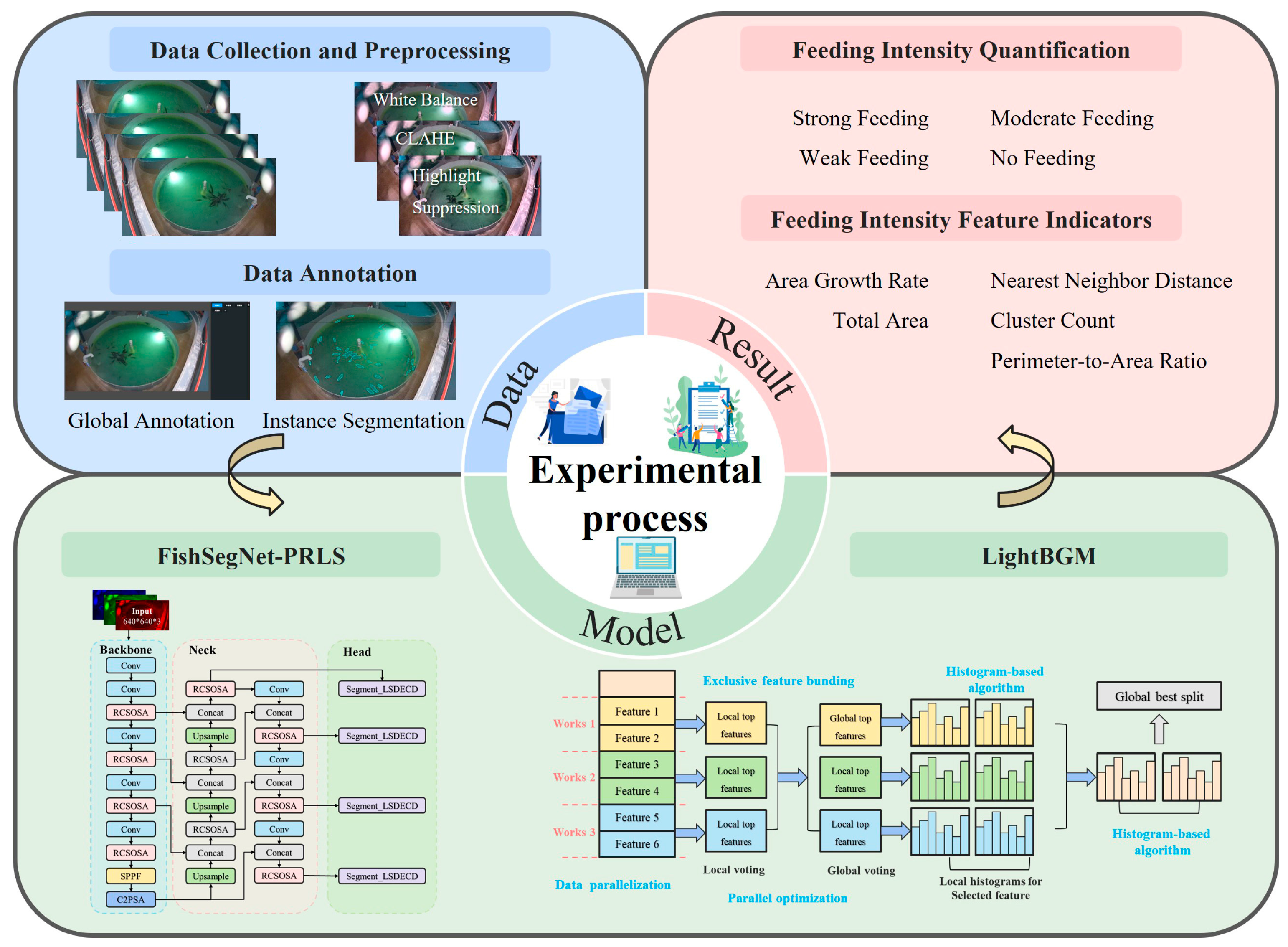
Figure 1. Framework for quantifying mandarin fish feeding behavior.
Fishes 10 00630 g001
Figure 2. Diagram of the recirculating aquaculture system.
Fishes 10 00630 g002
Figure 3. Examples from the mandarin fish school feeding state dataset.
Fishes 10 00630 g003
Figure 4. Preprocessing of fish school feeding images.
Fishes 10 00630 g004
Figure 5. Network architecture of FishSegNet-PRL.
Fishes 10 00630 g005
Figure 6. Network architecture of RCSOSA.
Fishes 10 00630 g006
Figure 7. Network structure of the module with the added P2 detection layer.
Fishes 10 00630 g007
Figure 8. Network architecture of LSDECD.
Fishes 10 00630 g008
Figure 9. Principle of LightGBM.
Fishes 10 00630 g009
Figure 10. Training results of the FishSegNet-PRL model.
Fishes 10 00630 g010
Figure 11. Dataset comparison.
Fishes 10 00630 g011
Figure 12. Comparison of Mainstream Models. Note: The first column shows the manually annotated original image, and the subsequent columns display the instance segmentation results generated by different models. The colors in the images are used solely to distinguish segmented regions and do not represent species classification.
Fishes 10 00630 g012
Figure 13. Feature plots of mandarin fish schools. Note: Shaded regions represent the predicted feeding intervals for individual features. Dashed intervals denote the ground-truth feeding intervals.
Fishes 10 00630 g013
Figure 14. Importance of fish school features. Note: (A) SHAP beeswarm plot illustrating the direction and magnitude of positive and negative feature impacts on prediction results. (B) Rose chart of feature importance showing which features the model considers most influential overall.
Fishes 10 00630 g014
Figure 15. Feeding intensity of fish schools. Note: The red, purple, and green regions correspond to strong, medium, and weak feeding phases, respectively. The red horizontal line indicates the feeding cessation threshold. The dashed intervals denote the ground-truth feeding intervals.
Fishes 10 00630 g015
Table 1. Sample records of mandarin fish feeding activities by date.
DateTimeFeeding AmountDateTimeFeeding Amount
23 June5:56Strong8 July5:22Medium
17:46Strong 17:12Strong
17:39Medium 17:10Medium
27 June5:21Medium17 July5:18Medium
5:44Strong 17:08Medium
16:59Medium 17:06Strong
2 July5:25Strong24 July5:30Strong
5:54Strong 17:17Medium
Table 2. Quantitative indices for feeding intensity.
Intensity IndexFormulaDefinition
Total area S = A u n i o n A R O I Total area represents the proportion of the area occupied by the fish school in each frame relative to the total area of the observation region; A R O I represents the total area of the observation region; A u n i o n represents the union area of all instances in this frame.
Nearest Neighbor Distance D N N = 1 n i , j d i s t ( i , j ) Nearest neighbor distance refers to the average distance between each individual in the fish school and its nearest neighbor; dist(i,j) is the Euclidean distance between individual i and j; n is the number of individuals in the calculation.
Area Growth Rate R g r o w t h = A t A t 1 t Area growth rate represents the rate of change in the fish school’s area over a unit of time; A t is the fish school area at the current time point; A t 1 is the fish school area at the previous time point; t is the time interval.
Cluster Count K t = N t Cluster count represents the number of valid clusters in the current frame; a cluster refers to a group of fish within the school that exhibits a certain degree of aggregation; N t represents the number of valid clusters in this frame (after removing small noise, non-fish instances, and instances outside the ROI).
Perimeter-to-Area Ratio P A = P A The perimeter-to-area ratio is the ratio of the fish school’s external contour perimeter (P) to the fish school’s area (A).
Table 3. Results of the ablation experiments.
ModelP2RCSOSALSDECDBox
P/%
Box
R/%
mAP
@50/%
mAP
@50–95/%
Mask
P/%
Mask
R/%
mAP
@50/%
mAP
@50–95/%
FPS
N1 7976.981.146.968.16466.227116.09
N2 8281.684.849.676.775.778.535.195.06
N3 79.275.980.246.168.965.467.928151.59
N4 80.776.981.646.968.465.566.627.4107.47
N5 80.680.884.85075.474.478.135.2128.01
N6 81.882.28651.477.874.579.135.490.13
N7 80.376.38146.469.965.367.627.8138.66
N882.880.185.750.678.574.779.435.6112.13
Disclaimer/Publisher’s Note: The statements, opinions and data contained in all publications are solely those of the individual author(s) and contributor(s) and not of MDPI and/or the editor(s). MDPI and/or the editor(s) disclaim responsibility for any injury to people or property resulting from any ideas, methods, instructions or products referred to in the content.