Construction and Comparison of Different Models to Forecast Central Fishing Grounds for Trawl Fishery Targeting Argentine Shortfin Squid (Illex argentinus) in the Southwest Atlantic

Abstract

The abundant Argentine shortfin squid resource plays a key role in the Patagonian Large Marine Ecosystem, the Polar Frontal Zone Ecosystem, and the South Atlantic Subtropical Gyre Ecosystem. In this article, we analyzed the annual and monthly changes in catch per unit effort (CPUE) of Argentine shortfin squid with a spatial resolution of 0.25° × 0.25° and constructed three ensemble learning and two deep learning fishing grounds forecasting models using catch information and spatial–temporal and marine environmental data. The results of the study were as follows: 1. From 2016 to 2021, Argentine shortfin squid in the Southwest Atlantic experienced notable interannual fluctuations, with the resource showing an increase and then remaining stable from 2016 to 2018, a decline in 2019, and a substantial increase from 2020 to 2021. Seasonally, CPUE was low from November to January, rose significantly from February to May, and declined in June; 2. The XGBoost model had the best overall performance among the three tree models, achieving an average of 68.86% accuracy, 70.19% F1-score; 3. In the 2021 actual production data validation, the Fusion ResNet18 model achieved an average production data accuracy of 74.47%, F1-score of 73.85%; the Fusion 3DResNet18 model achieved an average production data accuracy of 81.27%, F1-score of 82.43%. This indicates that convolutional neural networks, particularly 3D versions, are more suitable than decision tree-based ensemble models for predicting Argentine shortfin squid fishing grounds. Highly accurate fishing grounds forecasts help enterprises save production costs while providing some reference for the sustainable development of fishery resources.

1. Introduction

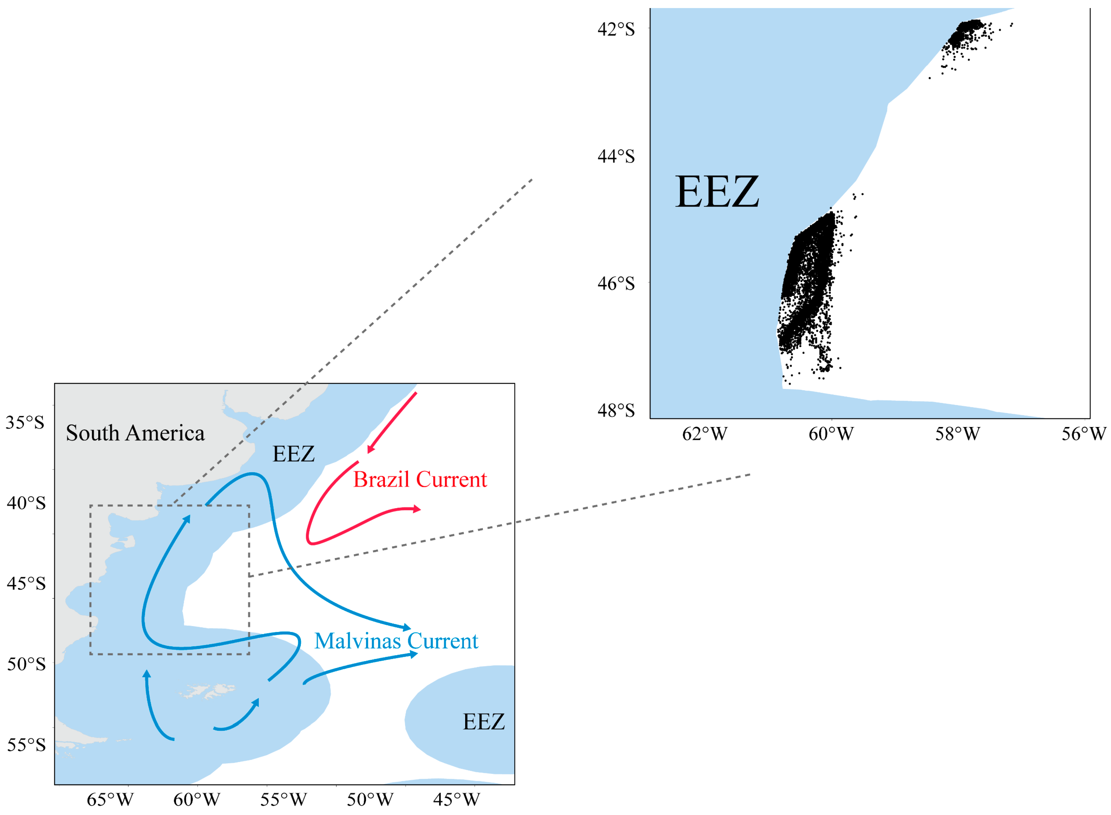
The current system formed by two opposing currents, the Brazil Current and the Malvinas Current, in the Southwestern Atlantic Ocean, is considered to be an essential influence on the resource abundance of the Argentine shortfin squid (Illex argentinus) (Figure 1) [1]. Argentine shortfin squid are characterized by a short life cycle, a rapid growth rate, a seasonal reproductive behavior, and only one reproduction throughout their life cycle [2]. The maturation period is 1 month for females and 1.5 to 2.5 months for males [3], with weight loss and reproductive atrophy at the beginning of the spawning cycle, followed by death once spawning is completed [4]. This reproductive characteristic determines that its population consists of almost a single generation, resulting in the variability in its resources depending mainly on the recruitment, and the dynamics of the Argentine shortfin squid fishery are closely linked to the changes in the marine environments. Various abiotic elements, such as water temperature, nutrient salts, currents, etc., may lead to fluctuations in the Argentine shortfin squid population [5]. It is primarily distributed in the Southwest Atlantic, between 23° S and 54° S, with the highest resource abundance occurring between 35°S and 52°S. Currently, it is widely believed that there are four spawning populations. The winter spawning group is the largest and is further divided into two subgroups: the Buenos Aires–Northern Patagonia group (Bonaerensis North Patagonian stock, BNPS), located north of 43° S, and the South Patagonia population (South Patagonian stock, SPS), located south of 44° S [6]. China’s share of world fisheries production has increased in recent decades [7]. In 2020, China became one of the significant contributors to the world’s capture fisheries. Meanwhile, the world capture production of Argentine shortfin squid is about 2.44 million tons, and this capture species is also an essential target for China’s pelagic fisheries. The Southwest Atlantic trawl fishery is the primary method for catching Argentine shortfin squid. The migration and movement of squid stocks require offshore fishing companies to continuously adjust the course of their vessels in search of key fishing grounds. High-accuracy fishing ground forecasts help companies reduce production costs while also providing valuable insights for the sustainable development of fishery resources.

Previous studies identified various factors affecting the ecology, resource status, and fishing grounds of the Argentine shortfin squid as latitude, sea surface temperature (SST), chlorophyll-a concentration (Chl-a), etc. Those studies were based on a generalized additive model (GAM) [8,9,10,11], multivariate linear model [12], maximum entropy model [13], Bayesian-based generalized linear model [14], Back Propagation (BP) neural network [15,16], and spatial overlay analysis [17]. Recent studies indicate a shift from traditional models to deep learning approaches in predicting Argentine shortfin squid fishing grounds. Researchers have shown that both environmental and spatiotemporal variables are key factors in modeling the distribution of this species. Among these, marine environmental variables are the most commonly used, with fluctuations in factors such as SST, sea surface height (SSH), and Chl-a directly or indirectly influencing squid abundance. These findings highlight the importance of incorporating environmental data into predictive models for more accurate forecasting of squid populations.

Fishing grounds refer to marine areas where fishing activities are concentrated due to the abundance of target species [18]. For Argentine shortfin squid, these fishing grounds are typically found in regions where environmental conditions, such as temperature and salinity, are favorable. Fishing grounds forecasting refers to predicting the distribution of fishing grounds or the spatial and temporal distribution of fishery resources based on existing statistics or environmental and fishery data. High-quality fishing grounds forecasts help fishery enterprises to rationalize production schedules and improve production efficiency [19]. The construction of the fishing grounds prediction model for Argentine shortfin squid in the Southwest Atlantic Ocean relies on the spatiotemporal and environmental elements of the study area such as the month, latitude and longitude, SST, sea surface salinity (SSS), dissolved oxygen (DO), etc. Researchers utilize the constructed prediction model to efficiently extract fishing ground features represented by these elements, and by integrating these with the inherent biological characteristics of the Argentine shortfin squid, they effectively analyze and forecast its spatiotemporal distribution and interannual variability in the Southwest Atlantic Ocean. As a species with a short life cycle, resource changes in Argentine shortfin squid are closely related to the marine environmental element. Establishing traditional fishing grounds forecasting models always depends on manually extracting marine environmental features. In contrast, the deep learning-based fishery forecasting model can make full use of the current conditions of computer arithmetic advancement, break the limitations of traditional ones, automatically extract the necessary information for fishery formation from big data, and improve the efficiency and accuracy of forecasting [20]. CPUE stands for catch per unit effort, which is a commonly used indicator in fisheries science to measure the relative abundance of a target species in a specific area. CPUE is relevant for forecasting fishing grounds because it reflects the density and distribution of target species in a given area. High CPUE values often indicate areas where the species is more abundant, making it a valuable metric for identifying potential fishing grounds. By analyzing the spatial and temporal variations in CPUE along with environmental variables, high-abundance fishing grounds can be effectively predicted.

The migration and relocation of fish stocks cause pelagic fishing companies to constantly modify fishing vessels’ routes to find the center fishing grounds during production. Therefore, the high accuracy of the fishing grounds forecast can help companies save production costs while providing some reference for the sustainable development of fishery resources. To better adapt to climate change and provide theoretical support for fishing grounds forecasting for Argentine shortfin squid in the Southwest Atlantic, as well as to inform the construction of fishing grounds forecasting models for other fish resources around the globe, this research aimed to (1) analyze annual and monthly CPUE changes in Argentine shortfin squid at 0.25° × 0.25° resolution; (2) construct three decision tree-based ensemble and two deep learning models using fishing logbooks, spatiotemporal, and environmental variables data. Meanwhile, they were validated with 2021 production data to identify the best model.

2. Materials and Methods

2.1. Study Area

The study area is located in the high seas of the Southwest Atlantic Ocean (45° W~61° W, 42° S~48° S, Figure 1), where the abundant resources of Argentine shortfin squid are attributed to the Malvinas Current and Brazil Current, and the convergence of the two currents provides favorable environmental conditions for the formation of the fishery. It is also the main production area for Chinese fishing vessels in the Southwest Atlantic Ocean.

2.2. Data Sources

2.2.1. Fisheries Data

The data on Argentine shortfin squid in the Southwest Atlantic Ocean used in this study came from the commercial fishing logbooks of Chinese trawlers in the Southwest Atlantic Ocean from the East China Sea and Pelagic Seas Data Service Center Database, which included vessel information (company name, port of registry, vessel model and equipment parameters, etc.), catch information (catch species, catch), operation information (date, number of nets, latitude and longitude, starting and releasing time of nets, etc.), and the original commercial fishing logbooks were categorized into two types: electronic version and paper version. The primary operating time for Argentine shortfin squid trawlers in the Southwest Atlantic was from November to June.

2.2.2. Marine Environmental Data

Combined with previous studies on the effects of environmental variables on the abundance of Argentine shortfin squid resources [17,21,22], a total of seven marine environmental variables were selected to construct the model in this study, namely, SST, SSH, Chl-a, SSS, mixed layer depth (Mlotst), DO, and 97 m water layer temperature (T97). The environmental variables data were inverted from satellite remote sensing data and derived from the Nucleus for European Modelling of the Ocean (NEMO) reanalysis values provided by Copernicus Marine Environmental Services (CMEMS, https://resources.marine.copernicus.eu/products (accessed on 23 November 2025)). The reanalysis values had a temporal resolution of months and a spatial resolution of 0.25° × 0.25°.

2.3. Fishery Data Preprocessing

The commercial fishing logbook operational information used in this study was recorded once a day for a total of 40, 576 fishery catch records. Fishery logbook records were curated by experienced fisheries experts to exclude non-fishing operations and correct obvious recording errors. To align the catch data with the spatial resolution of the environmental variables, the Southwest Atlantic was divided into 0.25° × 0.25° grid cells based on latitude and longitude. The operational position, total catch, and total nets were summarized monthly for each fishing area grid (time resolution). Based on this, CPUE was calculated with the formula:

$$\mathrm{C}\mathrm{P}\mathrm{U}\mathrm{E}={\displaystyle \frac{C_T}{Net}}$$

(1)

where $C_T$ is the total statistical catch (ton) in a 0.25° × 0.25° grid and Net is the total statistical nets (net) in a 0.25° × 0.25° grid in t/net. The resulting CPUE values formed a gridded CPUE dataset.

Gridded CPUE refers to the calculation of CPUE within specific spatial grid cells. In this study, the Southwest Atlantic was divided into 0.25° × 0.25° grid cells based on latitude and longitude. Within each grid cell, the total catch and total fishing effort (e.g., number of trawling hauls) for the same time period (e.g., monthly) were aggregated, and CPUE was calculated as the ratio of total catch to total effort. Gridded CPUE from 2016 to 2021 was grouped by year, based on which the median grid CPUE for each fishing area was further calculated based on each month of the year. The gridded CPUE of each fishing area was compared with the median of the corresponding month. Based on the results, the fishing grounds were classified into two categories. Specifically, if the gridded CPUE of a fishing ground was higher than the median of the month in which it was located, the fishing ground was defined as a central fishing ground; on the contrary, if the CPUE was lower than the median of the month, the fishing ground was identified as a non-central fishing ground.

2.4. Model Selection and Construction

2.4.1. Ensemble Learning Model

Random Forest (RF) Model

The RF model is an improved model proposed by Breiman based on the Bagging algorithm. It consists of multiple decision trees, each analyzing a subset of the dataset independently [23]. The RF model not only inherits the advantages of the Bagging parallel ensemble method but also has a higher generalization ability due to the significant flexibility of its sub-model, i.e., the decision boundary of the decision tree. Integrating multiple decision trees with significant individual differences can effectively reduce the errors that may be generated by a single decision tree, effectively solving the performance limitation problem caused by relying on a single decision tree and producing more accurate prediction results [24].

Extreme Gradient Boosting (XGBoost) Model

The XGBoost model, an optimization algorithm for gradient-boosted trees, was first proposed by Chen et al. in 2011 [25]. The XGBoost model constitutes an objective function based on a loss function and a regularization term. The loss function quantifies the accuracy of the model for fitting the data, while the regularization term draws a limit on the model complexity to reduce overfitting [26]. Meanwhile, the XGBoost model uses distributed parallel computing technology; the boosting algorithm is not easy to parallelize, but the XGBoost model parallelizes the computation in the feature column. The model training involves a large number of feature ordering and node-splitting calculations. The XGBoost model can calculate the gain of features in node splitting in parallel to speed up the model training [27].

Light Gradient Boosting Machine (LightGBM) Model

The LightGBM model is an efficient gradient boosting framework proposed to face large-scale data. Facing the challenge of large-scale data, traditional models based on boosting algorithms must traverse the entire training dataset several times in each iteration, which sets a high threshold for memory and computational resources. When the data cannot be loaded into memory at once, frequent disk read/write operations lead to serious efficiency degradation. The LightGBM model introduces two significant innovations on top of the traditional boosting algorithm-based model: histogram-based algorithm for optimality-seeking segmentation and leaf- wise growth strategy [28].

In addition, the LightGBM model introduces a gradient-based One-Side Sampling (GOSS) and a mutually exclusive feature merging technique [29]. The GOSS strategy prioritizes high-gradient instances and reduces computational and memory resource consumption by randomly sampling small gradient instances. In conjunction with the mutually exclusive feature merging technique, it further reduces data sparsity and computational burden and expands the ability to handle high-dimensional and large-scale data.

Ensemble Learning Modeling Model

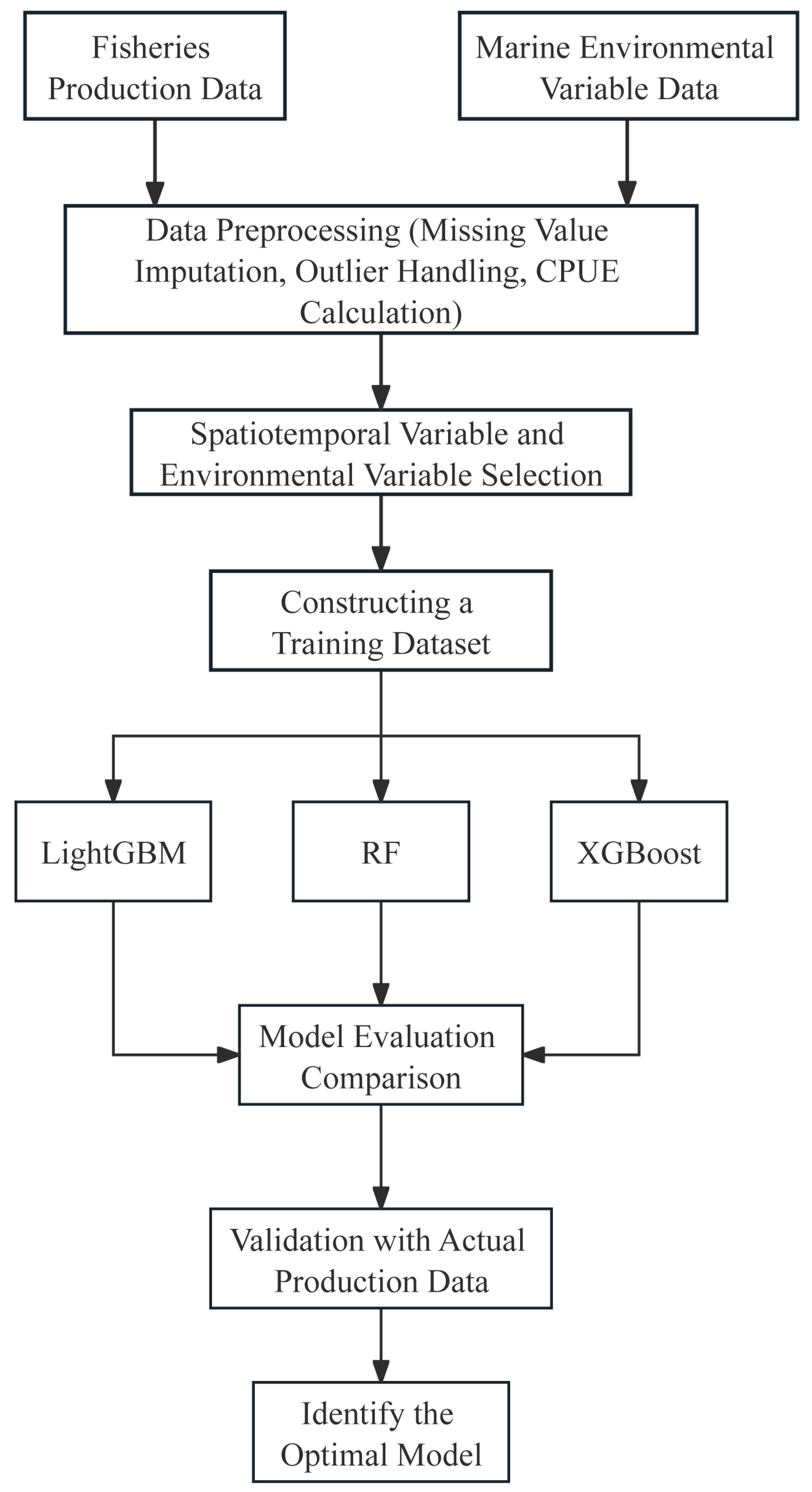
In this study, the training set in the dataset was first used to construct three different models, namely, RF, XGBoost, and LightGBM, respectively. To ensure reproducibility, all experiments were conducted with a fixed random seed of 42. Only three key hyperparameters, learning rate, max_depth, and n_estimators, were tuned for each model, while all other parameters retained their default values in XGBoost v2.0.2, LightGBM v4.1.0, and scikit-learn v1.2.1. The parameters of each model were optimized using grid search and five-fold cross-validation to screen out the best parameter settings (model parameter setting:

Table 1. Parameter settings in RF, XGBoost, and LightGBM models.

Model	Parameters	Range of Values
RF model	n_estimators	100, 150, 200, 250, 300, 350, 400, 450
	max_depth	6, 8, 10, 12, 14, 16
XGBoost model	n_estimators	100, 150, 200, 250, 300, 350, 400, 450
	max_depth	6, 8, 10, 12, 14, 16
	Learning rate	0.01, 0.05, 0.1
LightGBM model	n_estimators	100, 150, 200, 250, 300, 350, 400, 450
	max_depth	6, 8, 10, 12, 14, 16
	Learning rate	0.01, 0.05, 0.1

), and then the optimal model was obtained. Subsequently, the feature importance of the optimal model was output using the feature_importances_ function in the scikit-learn library, with a view to filtering and exploring the influence of environmental variables on the forecasting of the Argentine shortfin squid fishing grounds. Finally, the real production data in 2021 were used as a validation set to bring into the model for the simulation and validation of actual production scenarios, and model evaluation and comparison were carried out to obtain the optimal forecasting model. Figure 2 illustrates the ensemble learning fishing grounds forecasting model construction process.

2.4.2. Deep Learning Model

Convolutional Neural Networks and Residual Networks

A convolutional neural network is a network structure in deep learning technology, which mainly consists of a convolutional layer, pooling layer, and fully connected layer. The convolutional layer is the core of the model, and its main role is to perform spatial convolution operations to identify local features in the input data. On the other hand, the pooling layer reduces the feature dimensions by means of sampling, which reduces the model parameters and the amount of computation and also provides the model robustness to local variations. The fully connected layer is the integration of high-level abstract information for the final classification or regression task [20].

A 3D convolutional neural network operates in a similar essence to 2D convolution (two-dimensional convolution), but differs in its treatment of spatial dimensions. In 3D convolution, the convolution kernel slides in width and height and moves in the depth (or time) dimension. This means that the input data are a three-dimensional feature map, such as the width, height, and depth of a pixel point or the width, height, and time in a video. The convolution kernel is also a three-dimensional matrix, and by sliding over this feature map, features with depth information can be extracted [30].

Residual network (ResNet) is a deep learning model proposed by He et al. [31] and others in Microsoft Research. This model introduces the concept of “residual block” in the convolutional neural network model, which effectively solves the problem of gradient disappearance and gradient explosion in the traditional deep learning network and is able to better construct deep networks. The structure of a residual module typically consists of two main parts: the Main Path and the Residual Connection. The Main Path contains a series of layers such as convolution, pooling, and activation functions that are used to learn the feature representation of the input data. The Residual Connection, on the other hand, is responsible for summing the input data with the output of the Main Path, allowing the input to be passed directly to the output across the layers and passing the residual signals to the subsequent layers of the network. The introduction of the residual module allows certain layers to retain the information obtained from the model’s previous levels of learning even though no meaningful transformations are made, mitigating the problem of gradient vanishing.

Construction of the Dataset

Each sample in the dataset consists of three parts: the first part was a multi-channel multidimensional matrix containing a variety of marine environmental variables data; the second part was a one-dimensional matrix for storing spatiotemporal variables, including latitude, longitude, and month information; and the third part was the fishing grounds type labels, which were set to be 1 for the central fishing grounds labels and 0 for the non-central fishing grounds labels. In total, 80% of the data from 2016 to 2020 in the dataset were used as the training set, 20% as the validation set, and the 2021 data were used to test the model’s performance in the actual production environment.

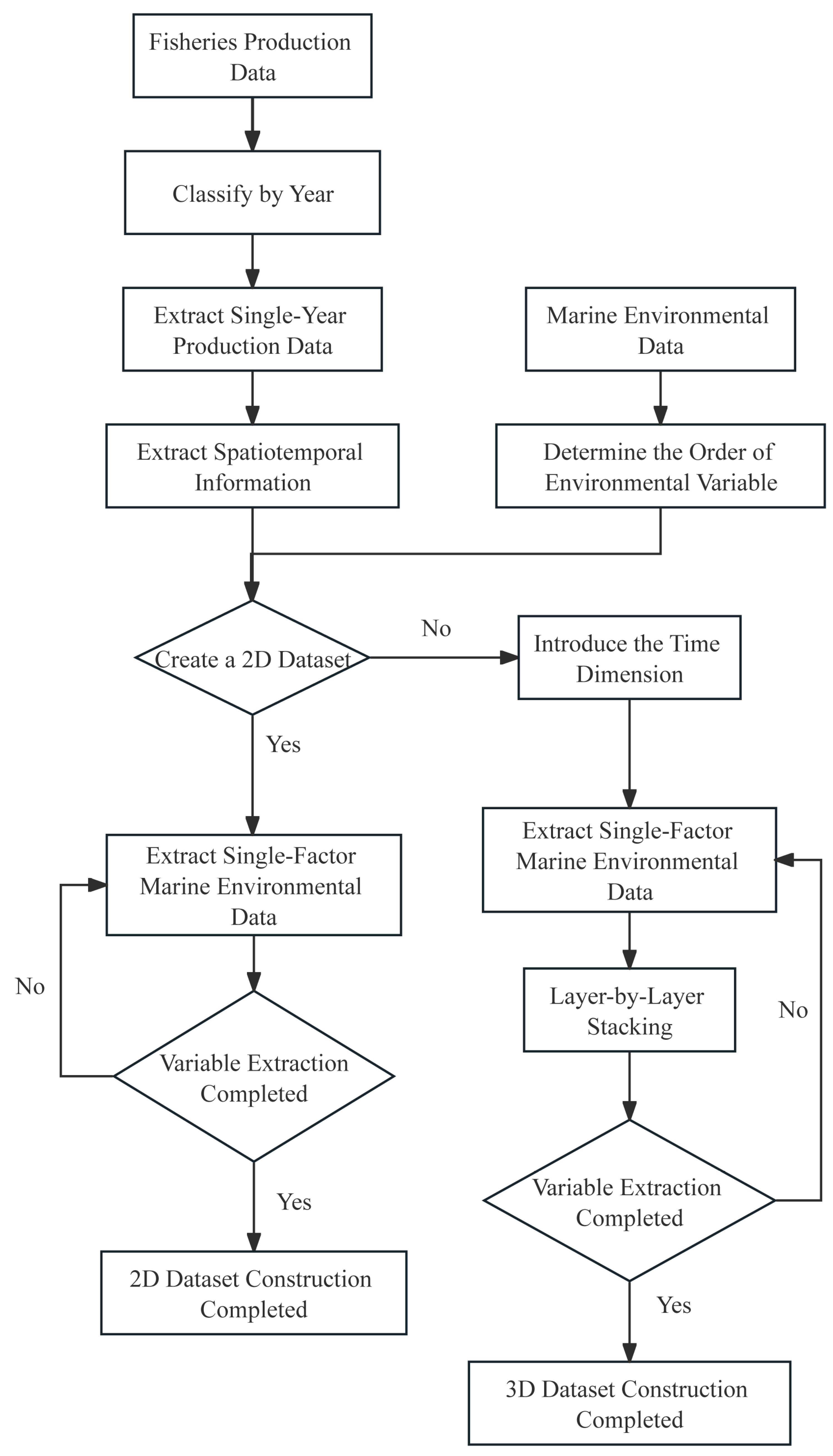
The dataset construction process in this section is shown in Figure 3: Firstly, the fishery data of Argentine shortfin squid and environmental variables data of Argentine shortfin squid were matched based on the operational time and latitude and longitude, and the surrounding marine environmental data were extracted centered on the latitude and longitude of the fishing area to form a 32 × 32 environmental data 2D matrix to construct a dataset. Subsequently, the 2D dataset was used as the basis to introduce the time dimension to construct the 3D dataset. The 32 × 32 environmental variables data of the month around the fishing area were first extracted as the basic information. Then, the environmental data were extracted toward the historical time dimension according to the preset step parameter for layer-by-layer stacking to form a complete time series. To ensure model consistency, the same order of environmental elements extraction was used in both the 2D and 3D dataset construction process, with the order of SST, SSH, T97, SSS, Mlotst, and Chl-a.

Model Construction

In this section, the ResNet model was chosen as the basis for constructing a forecast model for Argentine shortfin squid fishing grounds in the Southwest Atlantic.

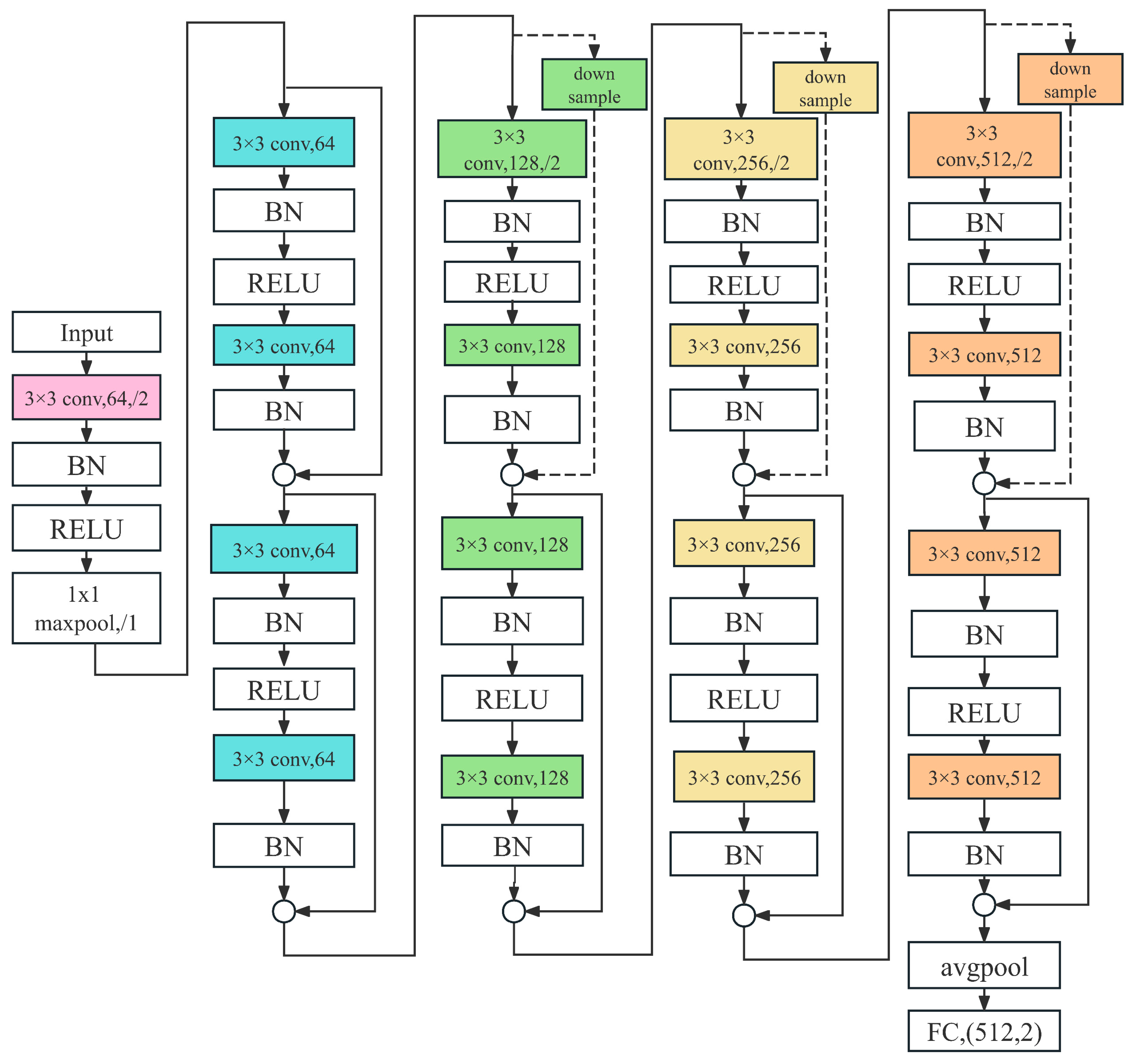
ResNet18 is a smaller version of the ResNet family [31] with fewer parameters and computational complexity, and contains the basic residual module. Figure 4 shows the structure of the ResNet18 model with an overall network depth of 18 layers, including 17 convolutional layers and 1 fully connected layer, excluding other layers. In the residual block, the layers were generally stacked in the order of “convolutional layer–BN layer–ReLU activation function”. The BN layer is a Batch Normalization layer, which normalizes the inputs of each layer so that they have a mean of 0 and variance of 1.

The model steps were as follows: Take ResNet18 as an example; firstly, the input data size of the model was 7 × 32 × 32, that is to say, 7 channels, the size of each channel was 32 × 32, and then entered the first convolutional layer, the size of the convolutional kernel was 3 × 3, the step size was 2, and the padding was 3. Then, passing through a maximal pooling layer, the size of the convolutional kernel was 1 × 1, the step size was 1, and the padding was 1. This was followed by a stack of eight residue blocks, where every two residue blocks were considered as a group, and there were four groups in total, each operating similarly. The size of the convolution kernel of the two residual blocks in the first group was 3 × 3, the step size was 1, and the padding was 1. The size of the data and the number of channels have not been changed. In the second, third, and fourth groups, the input data were divided into two branches inside the starting residual block of each group. In branch 1, the data passed through a 1 × 1 convolutional layer, which adjusted the number of channels of the feature map, followed by a convolutional operation set to a step size of 2 to perform down sampling to reduce the spatial dimension. Meanwhile, branch two directly applied a convolution with a step size of 2 to the output data of the previous layer, doubling the number of convolution kernels, and the rest of the convolution layers in the group had a step size of 1 and the same number of kernels as the previous convolution layer. After completing all the convolution operations, the fully connected layer was entered to integrate advanced features. Finally, the linear layer was entered to output the final prediction results of the model.

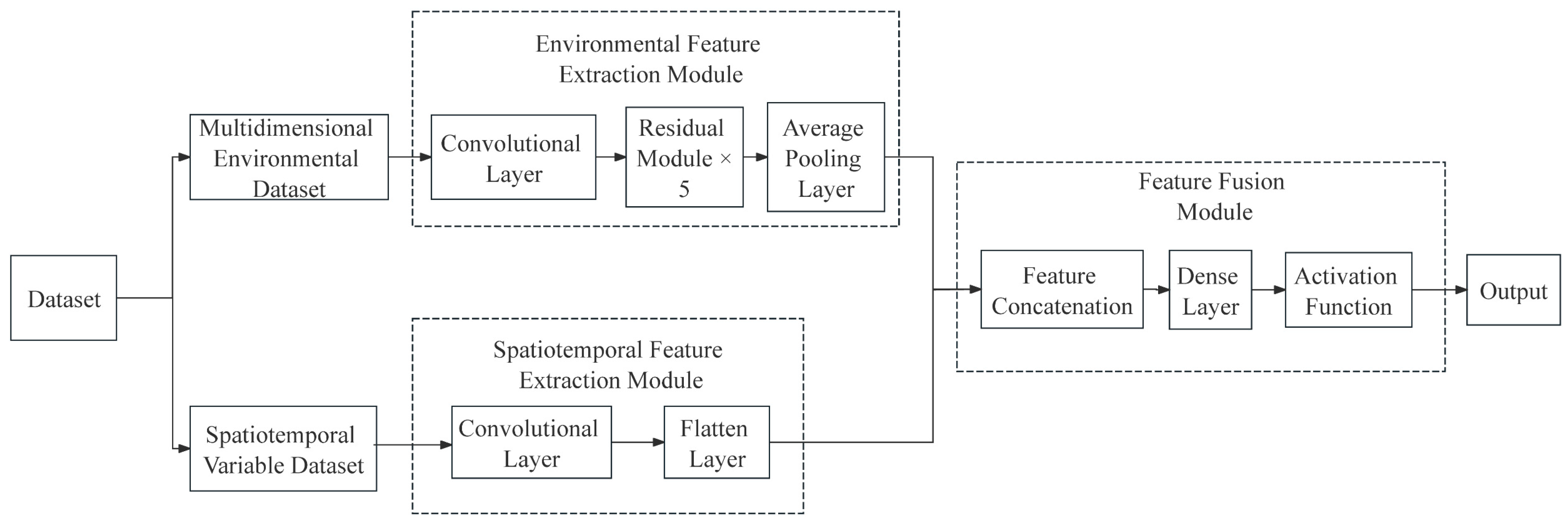
In order to make fuller use of the data, for the characteristics of spatiotemporal variables as a one-dimensional data structure, this paper used a one-dimensional convolutional neural network to map the spatiotemporal variables data into a high-dimensional feature set with more features, while using the ResNet network for feature extraction for multidimensional environmental data.

Experimental Process

The experiments in this chapter used Windows 11 as the operating system, Intel Core i7-12700 as the CPU model, and NVIDIA GeForce RTX 3060 as the GPU model. Based on this configuration, the Python3.8-based Pytorch 1.13.0 framework was built on the Anaconda3 platform. Model construction was performed for the 2D dataset and 3D dataset in the above experimental environment.

The model training process is shown in Figure 5, where the corresponding models were constructed for the 2D dataset and 3D dataset for training, and the models were named Fusion ResNet18 and Fusion 3DResNet18 because the models were based on ResNet18 with the addition of a 1D feature extraction module, respectively. The steps of model training were the same, and the first step was to combine the multidimensional environment firstly, the multidimensional environment dataset, and the spatiotemporal variables dataset were input into the corresponding feature extraction module, and the features extracted from the two modules were spliced together, and finally, the features were fused through the full connectivity layer to obtain the prediction results, and the output model evaluation indexes were used for the comparison of prediction effects.

2.5. Evaluation Criteria for Model Prediction Performance

In the process of model evaluation, accuracy is a commonly used evaluation metric, defined as the ratio between the number of samples correctly predicted and the total number of samples. In the context of this study, it referred to the ratio of the number of samples successfully predicted as central and non-central fishing grounds to the total number of samples, reflecting the model’s predictive ability in distinguishing between the two fishing grounds. The calculation formula was as follows:

$$\mathrm{A}\mathrm{c}\mathrm{c}\mathrm{u}\mathrm{r}\mathrm{a}\mathrm{c}\mathrm{y}={\displaystyle \frac{\mathrm{T}\mathrm{P}+\mathrm{T}\mathrm{N}}{\mathrm{T}\mathrm{P}+\mathrm{T}\mathrm{N}+\mathrm{F}\mathrm{P}+\mathrm{F}\mathrm{N}}}$$

(2)

where TP represented the number of fishing areas that were central fishing grounds in both the actual sample and the predicted results; FN refers to the number of fishing grounds that were central but predicted to be non-central fishing grounds; FP represents the number of fishing grounds that were actually non-central but incorrectly predicted to be central fishing grounds; and TN denoted the number of fishing areas that were actually and correctly predicted to be non-central fishing grounds.

For the Argentine shortfin squid fishing grounds forecasting model, a single evaluation metric cannot fully reflect the effectiveness of the model application, and the model’s precision, recall, and F1-score were also used as reference aids to evaluate the model’s effectiveness. Precision measures the proportion of correctly predicted fishing grounds that are predicted to center; recall represents the proportion of actual centers that are successfully predicted; and F1-score is a comprehensive measure of precision and recall. The formula is shown below as follows:

$$\mathrm{P}\mathrm{r}\mathrm{e}\mathrm{c}\mathrm{i}\mathrm{s}\mathrm{i}\mathrm{o}\mathrm{n}={\displaystyle \frac{\mathrm{T}\mathrm{P}}{\mathrm{T}\mathrm{P}+\mathrm{F}\mathrm{P}}}$$

(3)

$$\mathrm{R}\mathrm{e}\mathrm{c}\mathrm{a}\mathrm{l}\mathrm{l}={\displaystyle \frac{\mathrm{T}\mathrm{P}}{\mathrm{T}\mathrm{P}+\mathrm{F}\mathrm{N}}}$$

(4)

$$\mathrm{F}1-\mathrm{s}\mathrm{c}\mathrm{o}\mathrm{r}\mathrm{e}=\frac{2\times \mathrm{r}\mathrm{e}\mathrm{c}\mathrm{a}\mathrm{l}\mathrm{l}\times \mathrm{p}\mathrm{r}\mathrm{e}\mathrm{c}\mathrm{i}\mathrm{s}\mathrm{i}\mathrm{o}\mathrm{n}}{\mathrm{r}\mathrm{e}\mathrm{c}\mathrm{a}\mathrm{l}\mathrm{l}+\mathrm{p}\mathrm{r}\mathrm{e}\mathrm{c}\mathrm{i}\mathrm{s}\mathrm{i}\mathrm{o}\mathrm{n}}$$

(5)

3. Results

3.1. Variation in Annual and Monthly Mean CPUE of Argentine Shortfin Squid

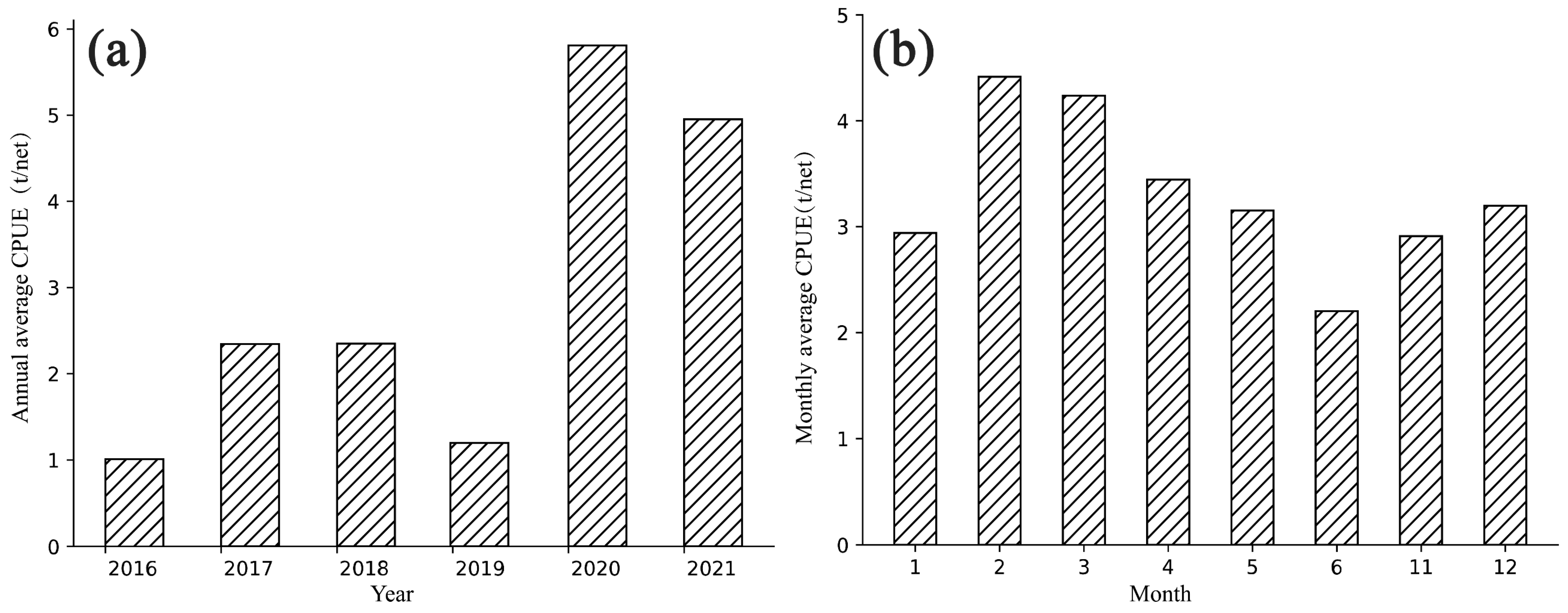
The total number of vessels and the total number of nets for 2016–2021 are shown in

Table 2. Total number of vessels and total number of nets from 2016 to 2021.

Year	Total Number of Vessels	Total Number of Nets
2016	20	3416
2017	27	6923
2018	30	8930
2019	27	4085
2020	25	7976
2021	29	9246

. As can be seen from Figure 6a, the annual average CPUE of Argentine shortfin squid in the Atlantic high seas waters fluctuates greatly, with the lowest and highest CPUEs in 2016 and 2020, respectively. The annual average CPUE rose rapidly from 2016 to 2018 and remained stable for two consecutive years. But in 2019, it rapidly declined to the level of 2016. From 2020 onwards, the annual average CPUE is historically high for two consecutive years, with 2020 in particular being the highest for the 2016–2021 period.

As can be seen from Figure 6b, the average monthly CPUE of Argentine shortfin squid in the Southwest Atlantic Ocean exceeded 2 t/net during the operational period, with a lower average monthly CPUE of 2.2 t/net in June, a relatively low average monthly CPUE from November to January, and the highest average monthly CPUE of 4.4 t/net in February.

3.2. Comparison of Ensemble Learning Models’ Prediction Performance

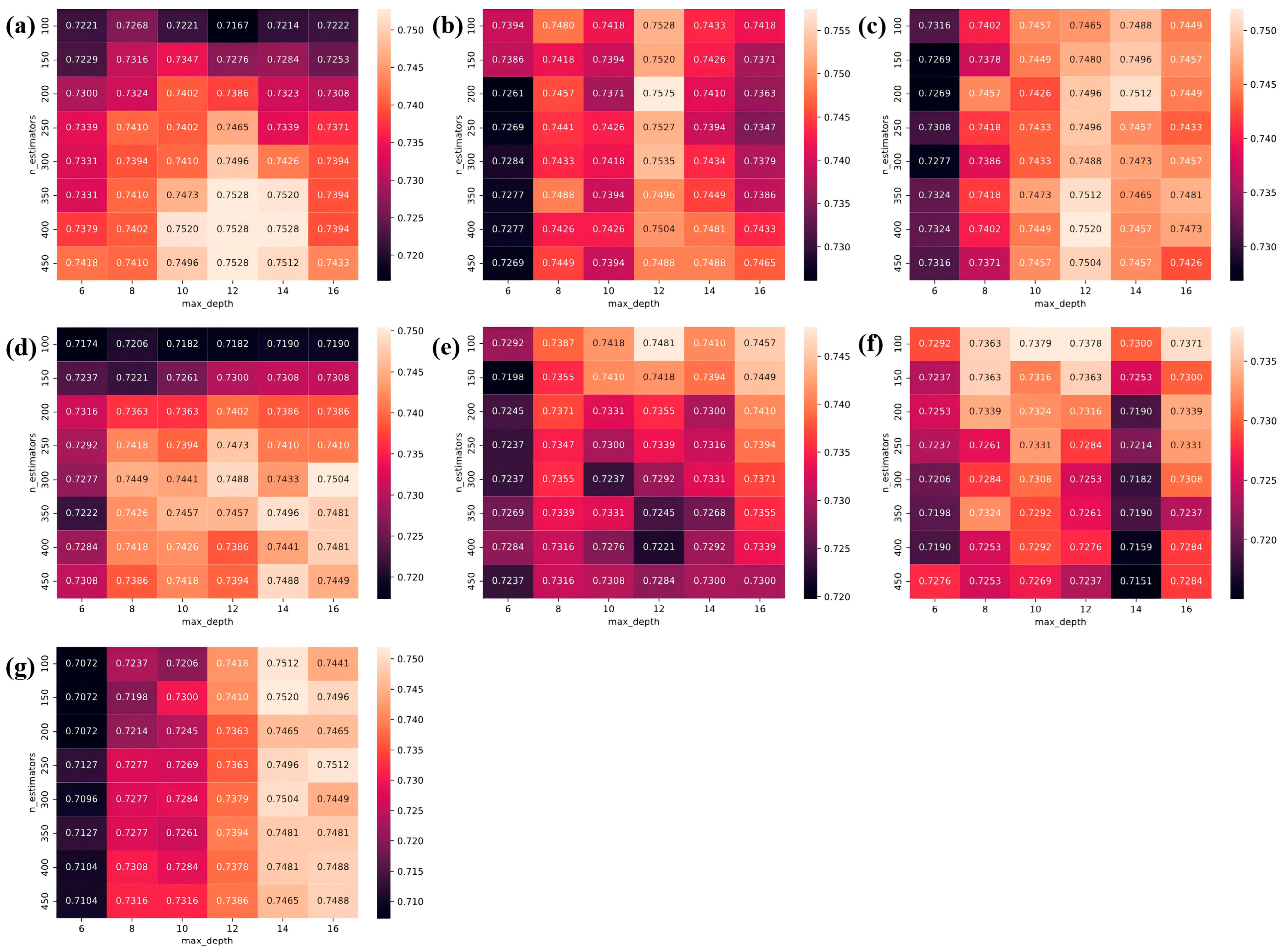
Figure 7 shows the cross-validation accuracy of XGBoost, LightGBM, and Random Forest across various hyperparameter combinations: XGBoost achieves the highest test accuracy (75.75%) at a learning rate of 0.05, max_depth = 12, and n_estimators = 200; Random Forest peaks at 75.20% with max_depth = 14 and n_estimators = 150; and LightGBM performs best (75.04%) when using a learning rate of 0.01, max_depth = 16, and n_estimators = 300. These parameter settings are therefore adopted as the final configurations for each model, respectively.

As can be seen from

Table 3. Comparison of prediction results of ensemble learning model.

Model	Precision (%)	Recall (%)	F1-Score (%)	Accuracy (%)
XGBoost	69.15	71.56	70.19	68.86
RF	68.97	58.82	63.49	65.67
LightGBM	65.93	59.12	62.17	63.68

, the XGBoost model exhibited optimal performance in terms of precision, recall, F1-score, and accuracy values of 69.15%, 71.56%, 70.19%, and 68.86%, respectively, in the validation experiments conducted for the actual production data in 2021. Compared with the XGBoost model, the performance of the RF model was relatively poor among the three models. Although the precision was close to that of XGBoost, the recall, F1-score, and accuracy were lower. The recall of the LightGBM model was slightly better than that of the RF model, but the precision, F1-score, and accuracy all performed slightly worse. Of the three models, neither the RF model nor the LightGBM model had a recall of more than 60%.

3.3. Feature Importance of the Optimal Model

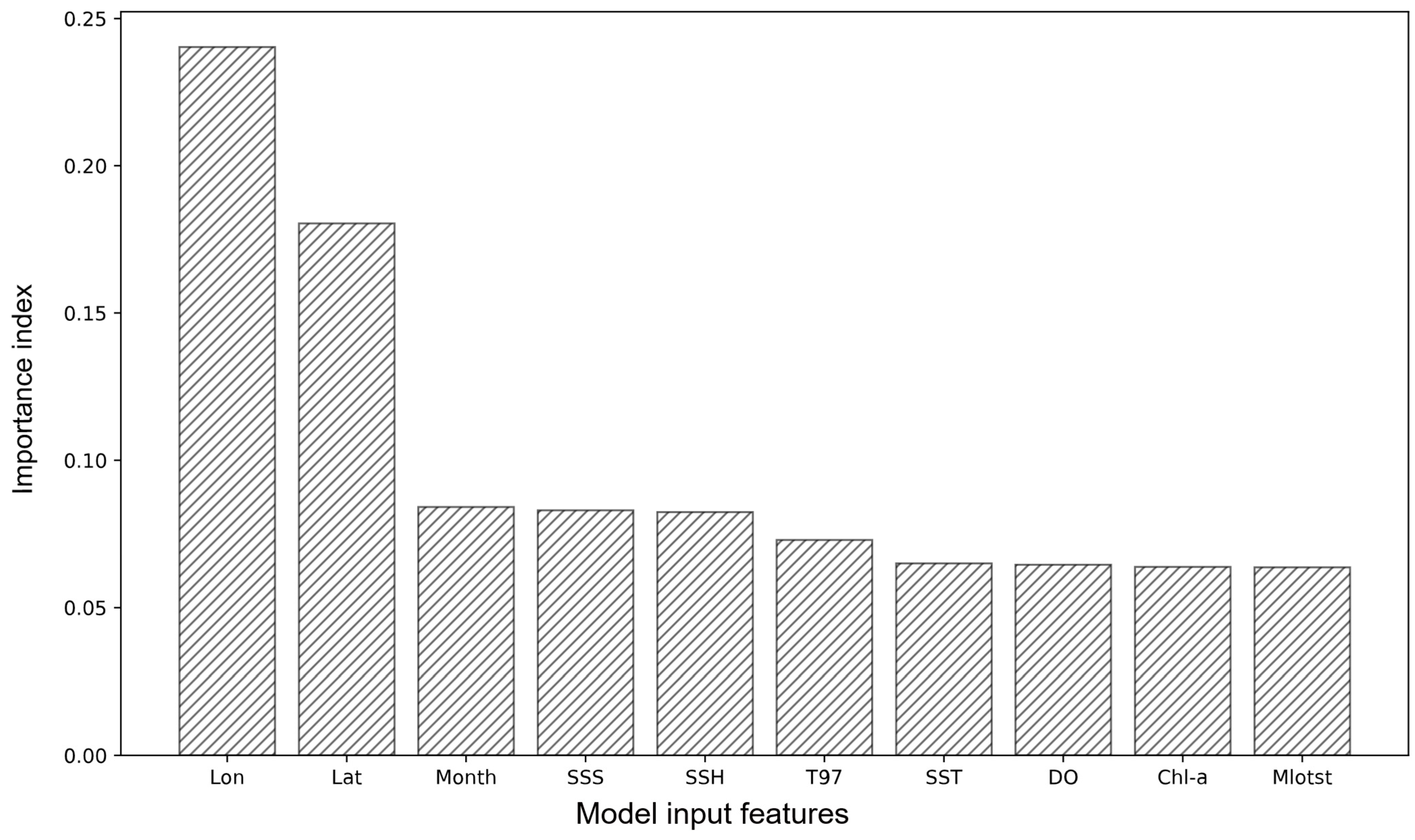
The XGBoost model exhibited the best overall performance among the three ensemble tree-based models, and thus its feature importance results are used for interpretation. As shown in Figure 8, the selected input features encompass spatiotemporal and environmental variables, all of which demonstrate non-negligible importance, indicating their collective influence on the formation and distribution of Argentine shortfin squid fishing grounds.

Longitude and latitude emerge as the most influential factors, reflecting the strong spatial dependence of squid habitat suitability. Month ranks third, highlighting seasonal variability in fishing ground dynamics. Among the environmental variables, SSS, SSH, T97, SST, DO, Chl-a, and Mlotst contribute progressively lower importance scores.

3.4. Comparison of Deep Learning Models’ Prediction Performance

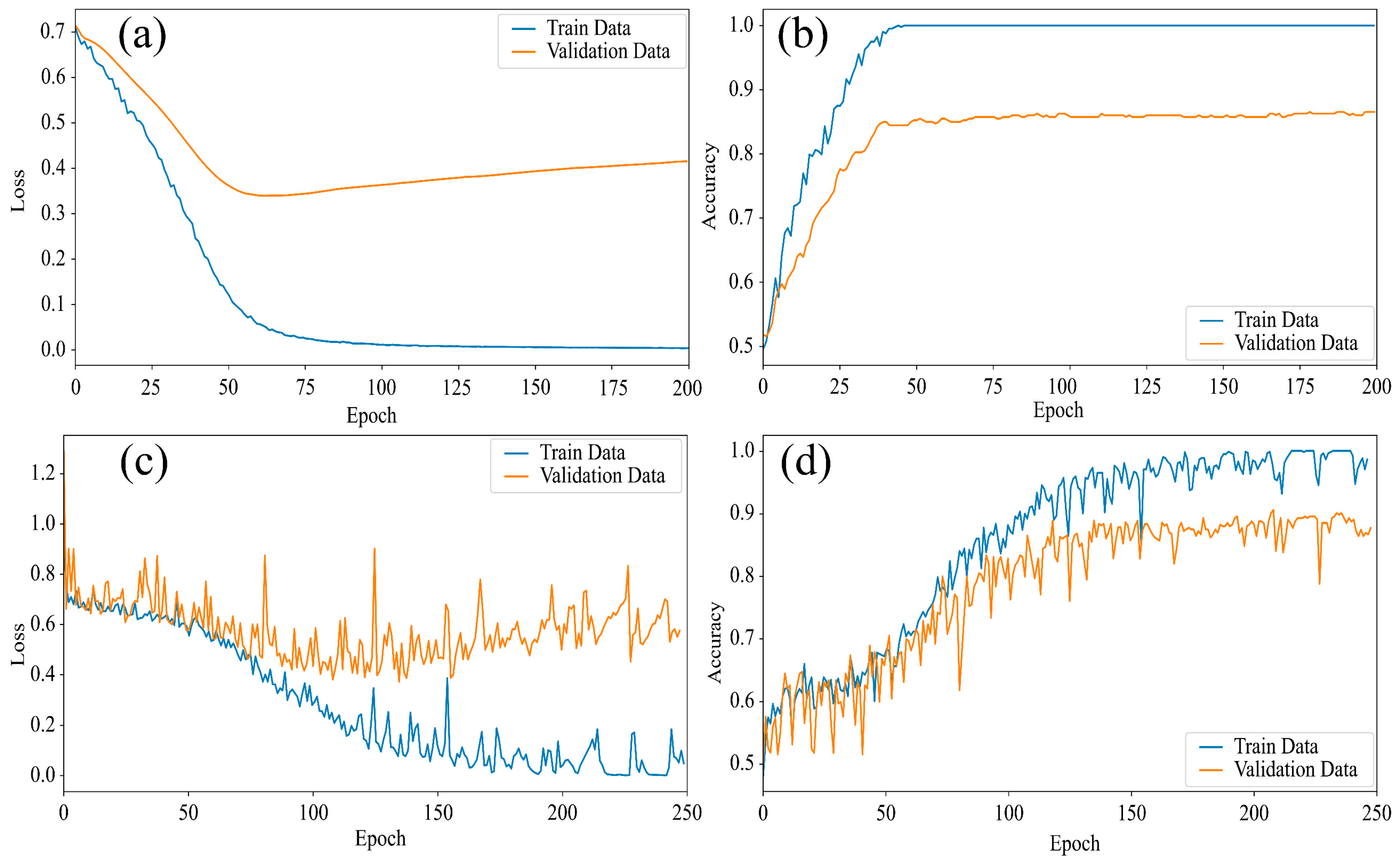
In the Fusion ResNet18 model, the number of iterations epoch was set to 200, the initial learning_rate was set to 0.0001, with a batch size of 8, and the optimizer used the Adam optimizer based on the Adam (Adaptive Moment Estimation) algorithm, which can adaptively adjust the learning rate. The model calculated the accuracy of the validation set once per iteration with the current model parameters. Figure 9a,b show the loss and accuracy of the Fusion ResNet18 model on the training and validation datasets, respectively, and the model’s accuracy on the validation set was up to 86.57% after the accuracy on the validation dataset was stabilized.

In the Fusion 3DResNet18 model, the number of model iterations epoch was 250, the initial learning rate was set to 0.0001, with a batch size of 8, the optimizer used the Adam function, and the model will compute the accuracy of the test set once with the current model parameters for each iteration, and Figure 9c,d show the loss and accuracy of the Fusion 3DResNet18 model on the training set and validation set, respectively. After the model stabilized on the test set, the accuracy on the test dataset was up to 90.79%.

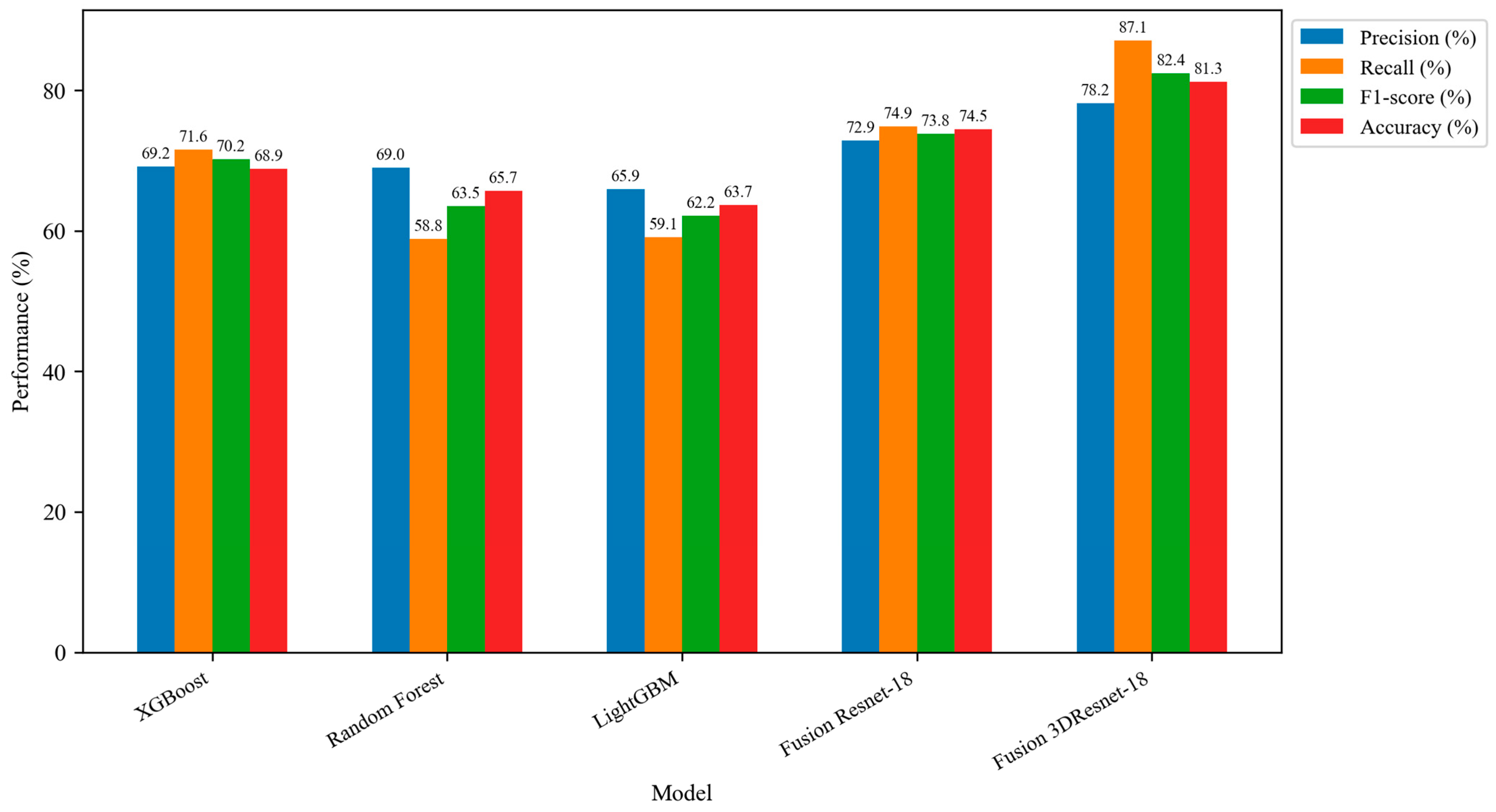
The 3D convolutional neural network-based Fusion 3DResNet18 model had improved in average accuracy, F1-score, precision, and recall compared to the 2D convolutional neural network-based Fusion ResNet18 model (

Table 4. Comparative analysis of the test dataset performance between Fusion Resnet-18 and Fusion 3DResnet-18 models.

Model	Precision (%)	Recall (%)	F1-Score (%)	Accuracy (%)
Fusion Resnet-18	72.87	74.86	73.85	74.47
Fusion 3DResnet-18	78.21	87.14	82.43	81.27

). The Fusion 3DResNet18 model had an average production data accuracy of 81.27%, an F1-score of 82.43%, a precision of 78.21%, and a recall of 87.14% for actual production data in 2021.

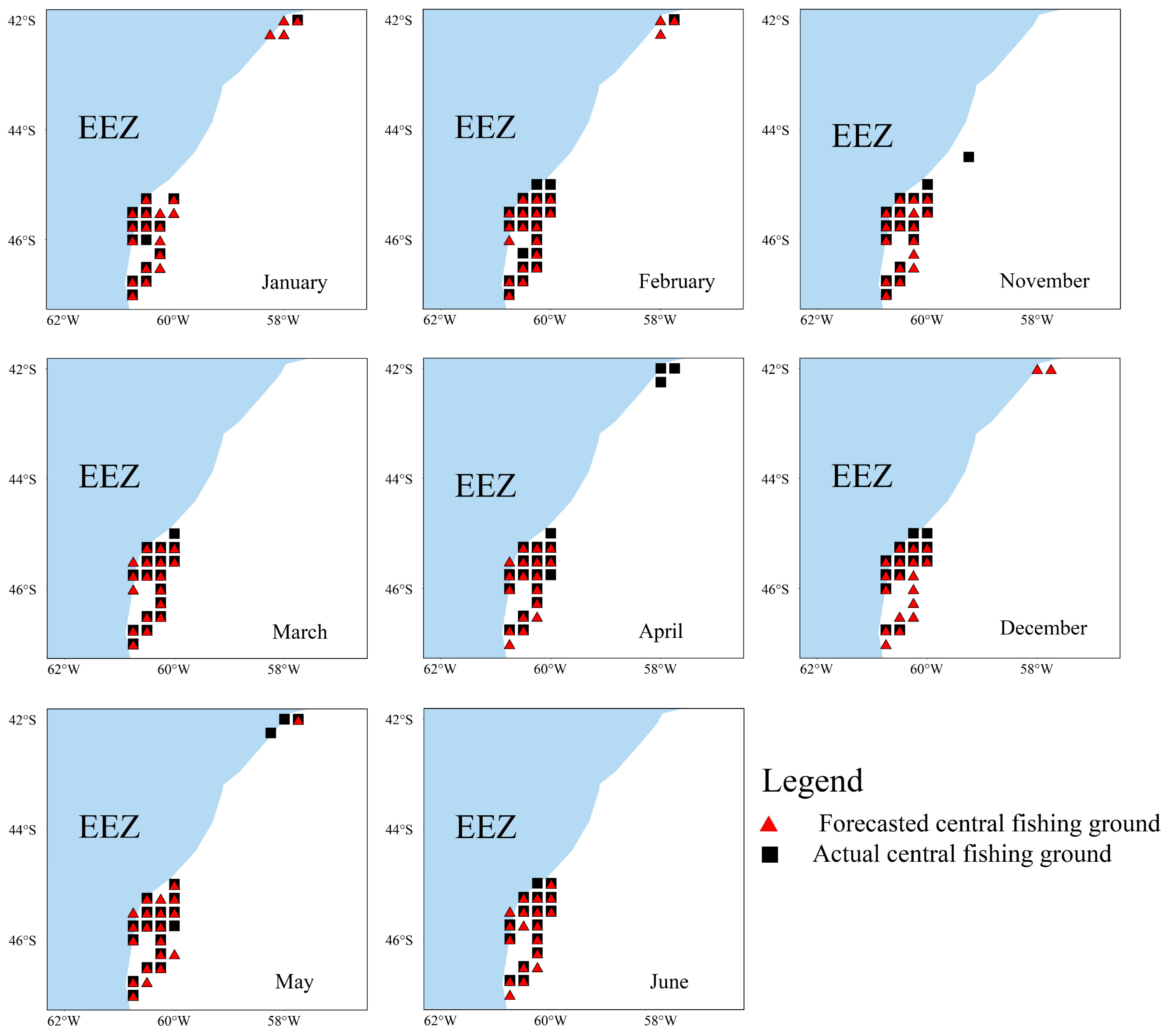
In order to verify the practical application of the model, based on the Fusion 3DResNet18 model, which had the highest forecast accuracy among the five Argentine shortfin squid fishing grounds forecasting models established by this institute (Figure 10), spatial and temporal data as well as environmental variables in 2021 were input into the trained 3DResNet18 model as a test dataset. Monthly forecasts of the Argentine shortfin squid fishing grounds in the Southwest Atlantic were made, and the forecast results were output. Since the location of the central fishing grounds is important for the actual production, we only visualized the difference in the location of the forecasted and actual central fishing grounds, and the results are shown in Figure 11. The center of the forecasted Argentine shortfin squid fishing grounds for each month in 2021 overlaps essentially exactly with the actual production center fishing grounds (Figure 11).

Based on the results obtained from the test dataset input model, the evaluation indexes were calculated, and the results are shown in

Table 5. Actual application effect of Fusion 3DResNet18 model in 2021.

Month	Precision (%)	Recall (%)	F1-Score (%)	Accuracy (%)
January	66.67	93.33	77.78	74.19
February	85.71	85.71	85.71	85.36
March	88.89	94.11	91.42	91.18
April	83.33	75.00	78.94	80.00
May	80.95	85.00	82.92	82.50
June	78.95	93.75	85.71	83.87
November	83.33	88.24	85.71	84.85
December	60.00	85.71	70.56	62.96

. The model showed good prediction performance in February–June and November, and slightly poorer prediction results in January and December, which need further optimization.

4. Discussion

4.1. Analysis of Changes in Annual and Monthly Average CPUE

Based on the operational production data of Argentine shortfin squid from 2016 to 2021, since 2017, the annual total number of nets has demonstrated significant differences despite the annual total number of fishing vessels remaining stable (Table 2). This suggests that there is not a positive relationship between the number of nets and the number of fishing vessels. This discovery revealed a significant interannual fluctuation in CPUE of Argentine shortfin squid, primarily attributed to the short lifespan of this species, which typically ranges around one year. Consequently, the abundance of Argentine shortfin squid resources is substantially influenced by the marine environment [11], especially through high seas trawl fishing, which was spreading Argentinean offshore continental shelf squid to the stocks at the high seas shelves and slopes. Therefore, the variation in its CPUE was large. Additionally, its stocks are also subject to resource variability in addition to changes in the marine environment that may lead to large changes in production [13,32].

The CPUE analysis revealed significant interannual fluctuations from 2016 to 2021. CPUE increased rapidly from 2016 to 2018, stabilized for two years, sharply declined in 2019, and peaked in 2020, maintaining high levels in 2021. These changes reflect the short life cycle of Argentine shortfin squid and environmental variability. Seasonally, CPUE was highest from February to May, the main fishing season, peaking in February and gradually declining by June. Lower CPUE values were recorded from November to January. Taken as a whole, the higher average monthly CPUE during the period from February to May can be considered as the main fishing season for the Argentine shortfin squid fishery.

Due to high exploitation rates and variable environmental conditions, the resource abundance of Argentine shortfin squid exhibits significant interannual fluctuations. From 2012 to 2013, the resource volume gradually recovered, and by 2014 to 2015, it had fully recovered. However, in 2016, the resource volume declined again, which may be related to the negative temperature anomaly of the bottom water in the southern part of the Patagonian continental shelf [12]. Statistical analyses of pelagic fishing logbooks [33] and GAM-based assessments of production data (2008–2018) [16] converged on identifying February–May as the critical fishing season for Argentine shortfin squid, despite variations in vessel operations. These findings align with the spatiotemporal patterns observed in the present study, thereby indicating a more pronounced seasonal fishing grounds in the species.

4.2. Comparative Analysis of Ensemble Learning Models

The XGBoost model had the best overall performance in predicting Argentine shortfin squid’s real fishing grounds in 2021. The performance of each index was better to some extent compared with the RF and LightGBM models. This may be because XGBoost uses a pre-sorting method to split the features and obtain the optimal splitting point by traversing all the splitting points [34]. On the other hand, to improve accuracy, the XGBoost model uses second-order gradient optimization and explicit regularization to mitigate overfitting, improve generalization ability, and increase model accuracy [35]. The RF model is created based on the Bagging algorithm by constructing multiple independent decision trees in parallel and finally integrating the training results as predictions. In contrast, its base learner shows higher flexibility in forming decision boundaries. This flexibility refers to the fact that only most of the features will be randomly extracted to construct the model when constructing branches in each tree of the RF model. With this strategy, independent decision trees may suffer from some limitations. However, this flexibility of the RF model reduces the single-tree error and breaks through the limitations of the performance of a single decision tree, giving it a higher generalization ability. Although this approach reduces the computational complexity and improves the training speed, the RF model mainly reduces the error by adding more trees. Compared with the gradient boosting tree, it does not directly optimize for the error, which may lead to unsatisfactory learning results when the model is more complex, and the training data are noisy [36,37]. The principle of the LightGBM model, although also based on the idea of boosting, improves the performance by iteratively adding new models; each new model is a correction of the error of the previous model. However, its main emphasis is on training speed and efficiency and its GOSS sampling method, which can be used to reduce the training complexity by filtering most of the small gradient samples without changing the data distribution. This allows the LightGBM model to have faster computational speed, better suppress the interference of noisy data, and perform well on big data. However, this practice of filtering samples may also result in filtered samples containing important information, leading to a degradation of model performance [29].

In this study, the fisheries dataset used is small compared to the large-scale datasets commonly used in traditional computer science and industry. Regarding data processing, the XGBoost model does not have the process of randomly discarding data, can fully utilize the data, and has good overfitting control. For both the RF and LightGBM models, there is some random selection and discarding process of data in the model construction process. Although all three ensemble learning algorithms present some utility in modeling the distribution of the Argentine shortfin squid fishing grounds, the XGBoost model showed the best results.

4.3. The Influence of Model Features on Fishing Grounds

Among the model input features, longitude and latitude exhibit the highest contribution scores, consistent with Sacau et al. [22], who reported spatial dominance using GAMs. This reflects both the influence of the Brazil–Malvinas Confluence, a key oceanographic feature that shapes Argentine shortfin squid fishing grounds by altering thermal and haline structures, and the fact that vessel positions in logbook-based fishery data likely track squid migration routes [9]. Seasonally, CPUE peaks from February to May, aligning with known temporal patterns of this species. SSS also plays a notable role, regional differences arise from mixing of distinct water masses [38], and salinity-driven osmoregulatory stress can affect squid metabolism and growth [17].

SSH acts as an indicator of current dynamics and vertical mixing, promoting nutrient upwelling and prey production under favorable conditions [39], while SST is consistently identified alongside SSH and spatial coordinates as a key predictor in prior studies [8]. T97 corroborates observations of Argentine shortfin squid aggregation near the 100 m layer [40]. DO supports the species’ high metabolic demands and influences spawning behavior [41,42], and Chl-a, as a proxy for primary productivity, shapes juvenile distribution through trophic availability [43,44]. Mlotst is critical for air–sea exchange and stratification [45] and has been shown to drive squid habitat formation in other regions [46].

4.4. Comparative Analysis of Deep Learning Models

The Fusion ResNet18 model uses a deep residual network technique, deepening the network model by solving gradient vanishing and explosion problems. This allows the network to handle more complex, high-dimensional datasets, such as the marine remote sensing environmental data used in this study, and thus to fit well and predict the Argentine shortfin squid fishing grounds. The Fusion ResNet18 model improves the average test accuracy of the Argentine shortfin squid fishing grounds prediction by 5.61% compared to the XGBoost model. It is demonstrated that using convolutional neural networks can extract the surrounding environmental features in marine remote sensing images, which can improve the effectiveness of fishing grounds prediction.

The dynamic nature of the marine environment is constant, and its indicators exhibit constant change over time. Marine organisms also migrate cyclically with time shifts, and for fisheries research, ignoring species’ changes in the temporal dimension may lead to difficult model fitting. Traditional 2D convolutional neural networks can extract marine environment feature information in the spatial dimension, but it is difficult to solve the problem of needing to integrate the time dimension. The 3D convolutional neural network not only extracts information in the spatial dimension but also incorporates the temporal dimension, allowing the model to more comprehensively extract features in both the temporal and spatial dimensions and identify species’ response to changes in the marine environment [47].

The Fusion 3DResNet18 model based on 3D convolutional neural networks showed an improvement in average accuracy, F1-score, precision, and recall compared to the 2D convolutional neural network Fusion ResNet18 model based on 2D convolutional neural networks, which demonstrates the ability of 3D convolutional neural networks in dealing with the problems with mixed spatial–temporal characteristics. The simultaneous increase in accuracy also indicates that including time dimension information allows the model to understand better and fit the changes in the marine environment and, thus, more accurately predict the Argentine shortfin squid fishing grounds.

5. Conclusions

This study constructed and compared three ensemble learning models (Random Forest, XGBoost, LightGBM) and two deep learning models (Fusion ResNet18 and Fusion 3DResNet18) for forecasting the central fishing grounds of Argentine shortfin squid in the Southwest Atlantic. Evaluation on 2021 production data demonstrated that the Fusion 3DResNet18 model achieved the best performance, with an accuracy of 81.27%, F1-score of 82.43%, precision of 78.21%, and recall of 87.14%. This represents an improvement over the best ensemble model (XGBoost: accuracy = 68.86%, F1-score = 70.19%) and the 2D deep learning counterpart (Fusion ResNet18: accuracy = 74.47%, F1-score = 73.85%). The performance of the 3D convolutional architecture confirms the importance of integrating temporal dynamics with spatial environmental features for predicting squid distribution. These forecasts can help fishing enterprises reduce operational costs and support sustainable fishery management in a changing ocean.

References

1. Liu, H.; Yu, W.; Chen, X. A review of Illex argentinus resources and the responses to environmental variability in the southwest Atlantic Ocean. J. Fish. Sci. China 2020, 27, 1254–1265. [Google Scholar] [CrossRef]
2. Lin, D.; Chen, X.; Chen, Y.; Fang, Z. Sex-specific reproductive investment of summer spawners of Illex argentinus in the southwest Atlantic. Invertebr. Biol. 2015, 134, 203–213. [Google Scholar] [CrossRef]
3. Arkhipkin, A.; Laptikhovsky, V. Seasonal and interannual variability in growth and maturation of winter-spawning Illex argentinus (Cephalopoda, Ommastrephidae) in the Southwest Atlantic. Aquat. Living Resour. 1994, 7, 221–232. [Google Scholar] [CrossRef]
4. Zang, N.; Lian, J.; Chen, X.; Lin, D. The yearly growth and body condition of Argentinean shortfin squid, Illex argentinus. Acta Hydrobiol. Sin. 2021, 45, 906–916. [Google Scholar] [CrossRef]
5. Chemshirova, I.; Hoving, H.-J.; Arkhipkin, A. Temperature effects on size, maturity, and abundance of the squid Illex argentinus (Cephalopoda, Ommastrephidae) on the Patagonian Shelf. Estuar. Coast. Shelf Sci. 2021, 255, 107343. [Google Scholar] [CrossRef]
6. Brunetti, N.E. Contribución al Conocimiento Biológico-Pesquero del Calamar Argentino (Cephalopoda: Ommastrephidae: Illex argentinus). Ph.D. Thesis, Universidad Nacional de La Plata, La Plata, Argentina, 1988. [Google Scholar]
7. FAO. The State of World Fisheries and Aquaculture; Food and Agriculture Organization of the United Nations: Rome, Italy, 2022; ISBN 978-92-5-136364-5. [Google Scholar]
8. Wang, J.; Chen, X.; Chen, Y. Projecting distributions of Argentine shortfin squid (Illex argentinus) in the Southwest Atlantic using a complex integrated model. Acta Oceanol. Sin. 2018, 37, 31–37. [Google Scholar] [CrossRef]
9. Chiu, T.-Y.; Chiu, T.-S.; Chen, C.-S. Movement patterns determine the availability of Argentine shortfin squid Illex argentinus to fisheries. Fish. Res. 2017, 193, 71–80. [Google Scholar] [CrossRef]
10. Chang, K.-Y.; Chen, C.S.; Wang, H.-Y.; Kuo, C.; Chiu, T. The Antarctic Oscillation index as an environmental parameter for predicting catches of the Argentine shortfin squid (Illex argentinus) Cephalopoda: Ommastrephidae) in southwest Atlantic waters. Fish. Bull. 2015, 113, 202–212. [Google Scholar] [CrossRef]
11. Chang, K.-Y.; Chen, C.-S.; Chiu, T.-Y.; Huang, W.-B.; Chiu, T.-S. Argentine Shortfin Squid (Illex argentinus) Stock Assessment in the Southwest Atlantic Using Geostatistical Techniques. Terr. Atmos. Ocean. Sci. 2016, 27, 281. [Google Scholar] [CrossRef]
12. Wang, Y.; Wang, J.; Chen, X.; Lu, H.; Lei, L. Interannual change of Illex argentinus abundance and its relationship with sea surface temperature in Falkland waters. Trans. Oceanol. Limnol. 2021, 43, 109–114. [Google Scholar] [CrossRef]
13. Chen, P.; Chen, X. Analysis of habitat distribution of Argentine shortfin squid (Illex argentinus) in the southwest Atlantic Ocean using maximum entropy model. J. Fish. China 2016, 40, 893–902. [Google Scholar] [CrossRef]
14. Lu, H.; Chen, X.; Cao, J. CPUE Standardization of Illex argentinus for Chinese Mainland squid-jigging fishery based on generalized linear Bayesian models. Acta Ecol. Sin. 2013, 33, 5375–5384. [Google Scholar] [CrossRef]
15. Li, N.; Lu, H.; Chen, X. Comparison of Different Forecasting Model for Fishing Ground of Illex argentinus Based on Artificial Neural Networks in the Southwest Atlantic Ocean. J. Guangdong Ocean Univ. 2017, 37, 65–71. [Google Scholar] [CrossRef]
16. Zhang, X.; Wang, J.; Chen, X. CPUE Standardization of Illex angentinus Based on BP Neural Network. Prog. Fish. Sci. 2022, 43, 11–20. [Google Scholar] [CrossRef]
17. Zhang, W.; Zhang, J. A discussion about relationship between the distribution of production of Illex argentinus and marine environmental factors in the Southwest Atlantic Ocean. J. Shanghai Ocean Univ. 2008, 17, 471–475. [Google Scholar]
18. Chen, X. Basic Theories of Formation of Fishing Ground. In Theory and Method of Fisheries Forecasting; Chen, X., Ed.; Springer Nature: Singapore, 2022; pp. 87–107. ISBN 978-981-19295-5-7. [Google Scholar]
19. Chen, X.; Gao, F.; Guan, W.; Lie, L.; Wang, J. Review of fishery forecasting technology and its models. J. Fish. China 2013, 37, 1270–1280. [Google Scholar] [CrossRef]
20. Han, H.; Jiang, B.; Shi, Y.; Jiang, P.; Zhang, H.; Shang, C.; Sun, Y.; Li, Y.; Xiang, D. Response of the Northwest Indian Ocean purpleback flying squid (Sthenoteuthis oualaniensis) fishing grounds to marine environmental changes and its prediction model construction based on multi-models and multi-spatial and temporal scales. Ecol. Indic. 2023, 154, 110809. [Google Scholar] [CrossRef]
21. Wu, Y.; Yang, S.; Shen, J.; Zhou, W.; Zhang, J. Fishing grounds characteristics of Illex argentinus in southwest Atlantic. Chin. J. Appl. Ecol. 2009, 20, 1445–1451. [Google Scholar] [CrossRef]
22. Sacau, M.; Pierce, G.J.; Wang, J.; Arkhipkin, A.I.; Portela, J.; Brickle, P.; Santos, M.B.; Zuur, A.F.; Cardoso, X. The spatio-temporal pattern of Argentine shortfin squid Illex argentinus abundance in the southwest Atlantic. Aquat. Living Resour. 2005, 18, 361–372. [Google Scholar] [CrossRef]
23. Breiman, L. Random Forests. Mach. Learn. 2001, 45, 5–32. [Google Scholar] [CrossRef]
24. Min, J.; Lu, T.; Ren, T.; Chen, R. Interpretable Machine Learning Algorithm Based on Rules Ensemble and Its Application. J. Front. Comput. Sci. Technol. 2024, 18, 1476–1490. [Google Scholar] [CrossRef]
25. Li, W.; Yin, Y.; Quan, X.; Zhang, H. Gene Expression Value Prediction Based on XGBoost Algorithm. Front. Genet. 2019, 10, 1077. [Google Scholar] [CrossRef]
26. Ding, X. Empirical Reasearch on ESG Multi-factor Model Based on XGBoost and Other Boosting Algorithms. Master’s Thesis, Shandong University, Jinan, China, 2024. [Google Scholar]
27. Ji, X. Research on Ship Risk Assessment Model Based on Machine Learning. Master’s Thesis, Zhejiang Ocean University, Zhoushan, China, 2023. [Google Scholar]
28. Li, B. Position determination algorithm for intelligent unmanned vehicles based on LightGBM model assistance. Master’s Thesis, Lanzhou Jiaotong University, Lanzhou, China, 2024. [Google Scholar]
29. Ke, G.; Meng, Q.; Finley, T.; Wang, T.; Chen, W.; Ma, W.; Ye, Q.; Liu, T.-Y. LightGBM: A highly efficient gradient boosting decision tree. In Proceedings of the Advances in Neural Information Processing Systems 30 (NIPS 2017), Long Beach, CA, USA, 4–9 December 2017. [Google Scholar]
30. Han, H.; Jiang, B.; Xiang, D.; Shi, Y.; Liu, S.; Shang, C.; Zhao, X.; Zhang, H.; Sun, Y. Comparison of model selection and data bias on the prediction performance of purpleback flying squid (Sthenoteuthis oualaniensis) fishing ground in the Northwest Indian Ocean. Ecol. Indic. 2024, 158, 111526. [Google Scholar] [CrossRef]
31. He, K.; Zhang, X.; Ren, S.; Sun, J. Deep Residual Learning for Image Recognition. In Proceedings of the IEEE Conference on Computer Vision and Pattern Recognition, Las Vegas, NV, USA, 27–30 June 2016; pp. 770–778. [Google Scholar]
32. Li, N.; Chen, X.; Wang, R. Incorporating spatial autocorrelation into CPUE standardization with an application to the Illex argentinus. Haiyang Xuebao 2018, 40, 61–68. [Google Scholar] [CrossRef]
33. Cui, G.; Xuan, W.; Wei, Q.; Tao, Y.; Su, S.; Yu, Q.; Zhu, W. Temporal and Spatial Variation of Illex argentinus Fishing Ground in the Southwest Atlantic Ocean Based on SST and Chl-a. J. Zhejiang Ocean Univ. Sci. (Nat. Sci.) 2023, 42, 10–19. [Google Scholar] [CrossRef]
34. Li, Z.; Liu, Z. Feature selection algorithm based on XGBoost. J. Commun. 2019, 40, 101–108. [Google Scholar] [CrossRef]
35. Zhou, W.-F.; Wang, J.-G.; Deng, L.-F.; Yao, Y.; Liu, J.-L. Terminal Temperature Prediction of Molten Steel in VD Furnace based on XGBoost and LightGBM Algorithms. In Proceedings of the 2021 IEEE 40th Chinese Control Conference (CCC), Shanghai, China, 26–28 July 2021; pp. 6289–6294. [Google Scholar]
36. Ren, S.; Zhao, W.; Zhou, X.; Sun, J. Global refinement of random forest. In Proceedings of the IEEE Conference on Computer Vision and Pattern Recognition, Boston, MA, USA, 7–12 June 2015; pp. 723–730. [Google Scholar]
37. Abellán, J.; Mantas, C.J.; Castellano, J.G. A Random Forest approach using imprecise probabilities. Knowl.-Based Syst. 2017, 134, 72–84. [Google Scholar] [CrossRef]
38. Zhang, X. Consideration of Heterogeneity of Fishery Data for Standardizing CPUE of Illex angentinus in Atlantic Ocean. Master’s Thesis, Shanghai Ocean University, Shanghai, China, 2022. [Google Scholar]
39. Guanyu, H.; Xinjun, C.; Jintao, W. Forecasting fishing ground of Illex argentinus based on different weight habitat suitability index in the southwestern Atlantic. Haiyang Xuebao 2015, 37, 88–95. [Google Scholar] [CrossRef]
40. Bazzino, G.; Quiñones, R.A.; Norbis, W. Environmental associations of shortfin squid Illex argentinus (Cephalopoda: Ommastrephidae) in the Northern Patagonian Shelf. Fish. Res. 2005, 76, 401–416. [Google Scholar] [CrossRef]
41. Roberts, M.J. Chokka squid (Loligo vulgaris reynaudii) abundance linked to changes in South Africa’s Agulhas Bank ecosystem during spawning and the early life cycle. ICES J. Mar. Sci. 2005, 62, 33–55. [Google Scholar] [CrossRef]
42. Wang, D.; Yao, L.; Yu, J.; Chen, P. The role of environmental factors on the fishery catch of the squid uroteuthis chinensis in the pearl river estuary, China. J. Mar. Sci. Eng. 2021, 9, 131. [Google Scholar] [CrossRef]
43. González, A.F.; Trathan, P.N.; Yau, C.; Rodhouse, P.G. Interactions between oceanography, ecology and fishery biology of the ommastrephid squid Martialia hyadesi in the South Atlantic. Mar. Ecol. Prog. Ser. 1997, 152, 205–215. [Google Scholar] [CrossRef][Green Version]
44. Anderson, C.I.; Rodhouse, P.G. Life cycles, oceanography and variability: Ommastrephid squid in variable oceanographic environments. Fish. Res. 2001, 54, 133–143. [Google Scholar] [CrossRef]
45. An, Y.-Z.; Wang, H.-Z.; Chen, Y.-D. Study on calculation and spatio-temporal variations of global ocean mixed layer depth. Chin. J. Geophys. 2012, 55, 2249–2258. [Google Scholar] [CrossRef]
46. Yu, W.; Chen, X.; Yi, Q. Analysis of variations in the environmental conditions on the fishing ground of neon flying squid (Ommastrephes bartramii) in the Northwestern Pacific Ocean under different climate modes. J. Fish. China 2017, 41, 525–534. [Google Scholar] [CrossRef]
47. Han, H.; Yang, C.; Jiang, B.; Shang, C.; Sun, Y.; Zhao, X.; Xiang, D.; Zhang, H.; Shi, Y. Construction of chub mackerel (Scomber japonicus) fishing ground prediction model in the northwestern Pacific Ocean based on deep learning and marine environmental variables. Mar. Pollut. Bull. 2023, 193, 115158. [Google Scholar] [CrossRef]
Figure 1. Spatial distribution of catch points of Argentine shortfin squid in the Southwest Atlantic, 2016–2021 (EEZ: Exclusive Economic Zone).
Fishes 10 00610 g001
Figure 2. Construction process of fishing grounds forecast model based on ensemble learning.
Fishes 10 00610 g002
Figure 3. Workflow of building deep learning dataset.
Fishes 10 00610 g003
Figure 4. ResNet18 model structure diagram.
Fishes 10 00610 g004
Figure 5. Training process flowchart of Fusion ResNet18 and Fusion 3DResNet18 models.
Fishes 10 00610 g005
Figure 6. Annual (a) and monthly (b) average CPUE distributions of Argentine shortfin squid in the Southwest Atlantic, 2016–2021.
Fishes 10 00610 g006
Figure 7. Grid search accuracy over n_estimators and max_depth: (ac) XGBoost with learning rates 0.01, 0.05, and 0.1; (df) LightGBM with learning rates 0.01, 0.05, and 0.1; (g) Random Forest.
Fishes 10 00610 g007
Figure 8. Relative importance of environmental features in the optimal XGBoost model.
Fishes 10 00610 g008
Figure 9. Loss and accuracy curves of Fusion ResNet18 and Fusion 3DResNet18 models on training and validation datasets. (a,b) Loss and accuracy for Fusion ResNet18; (c,d) loss and accuracy for Fusion 3DResNet18.
Fishes 10 00610 g009
Figure 10. Performance comparison of all candidate models across four evaluation metrics.
Fishes 10 00610 g010
Figure 11. Comparison between the actual central fishing grounds and the forecasted central fishing grounds in 2021 based on the Fusion 3DResNet18 model.
Fishes 10 00610 g011