Article

Spatiotemporal and Environmental Effects on Demersal Fishes Along the Nearshore Texas Continental Shelf

by
Erin M. Johnson
1,*,
Fernando Martinez-Andrade
2,
P. Santiago Domínguez-Sánchez
1,
Aurora Gaona-Hernandez
1,
Chengxue Li
1 and
R. J. David Wells
1
1
Department of Marine Biology, College of Marine Sciences and Maritime Studies, Texas A&M University, Galveston, TX 77553, USA
2
Texas Parks and Wildlife Department, Coastal Fisheries Division, Corpus Christi, 78418 TX, USA
*
Author to whom correspondence should be addressed.
Fishes 2025, 10(12), 632; https://doi.org/10.3390/fishes10120632
Submission received: 3 November 2025 / Revised: 4 December 2025 / Accepted: 5 December 2025 / Published: 9 December 2025
(This article belongs to the Section Biology and Ecology)

Abstract

The goal of this study was to analyze data from a 10-year bottom longline survey to examine spatial, temporal, and environmental effects on demersal fishes along the Texas coast within the northwestern Gulf of Mexico. Generalized additive models (GAMs) and generalized linear models (GLMs) were employed to evaluate trends and patterns in species composition (species richness and species diversity), relative abundance, and presence probability of fish species in the Texas region of the northwestern Gulf of Mexico. Temperature, salinity, and dissolved oxygen were the most influential variables driving richness, diversity, and abundance of demersal fish assemblages. The community was dominated by six species that represent 93% of total catch: Rhizoprionodon terraenovae (Atlantic sharpnose shark), Bagre marinus (gafftopsail catfish), Sciaenops ocellatus (red drum), Carcharhinus limbatus (blacktip shark), Carcharhinus brevipinna (spinner shark), and Carcharhinus leucas (bull shark). Analyses of dominant species revealed that multiple factors modulated their presence probability, with temperature and dissolved oxygen as common environmental drivers among species. Findings from the present study suggest that the composition and abundance of demersal fish assemblages were shaped by key environmental drivers.
Key Contribution: This multiyear assessment highlights the role of environmental variables as key drivers to shape composition and abundance of demersal fish assemblages. The assessment also corroborates the benefits of long-term monitoring programs in analyzing patterns and trends of marine species.

Graphical Abstract

1. Introduction

Environmental conditions in marine environments vary due to numerous natural and anthropogenic variables. These variables can underpin the dynamic nature of species composition and abundance—metrics often used to evaluate ecosystem health [1,2]. Water temperature and salinity are key environmental variables that affect fish biology (e.g., growth) and ecology (e.g., recruitment) and shape the spatiotemporal abundance of fish communities in coastal areas [3,4,5].
The Gulf of Mexico (hereafter referred to as GoM), one of the most ecologically and economically productive marine ecosystems in the United States, has been experiencing climate-driven changes in local water temperature and salinity, which, in turn, alter the structure of coastal communities [6,7,8]. For example, a recent study found expansion of tropical species into the northern GoM—due to rising water temperature—that resulted in enhanced regional fish diversity [9]. These findings are consistent with broader global observations of climate-driven range shifts in marine species [4]. In addition to temperature, variability in salinity and dissolved oxygen in the GoM coastal areas where freshwater inputs and eutrophication are frequent can also influence species diversity and community composition [10]. Although the influence of environmental factors on coastal fish communities in the broader GoM has been extensively studied, relatively little research has focused on the interplay of environmental drivers and the relative contributions to fish community structure along the nearshore continental shelf of the Texas coast within the northwestern GoM, due to limited availability of long-term ecological time series data.
Data from consistent, long-term monitoring programs can be used to elucidate patterns or anomalous changes in species composition and abundance concurrent to changes in environmental metrics due to natural or anthropogenic pressures [11]. For example, researchers have been monitoring effects of the annual hypoxia event on fish ecology since the 1970s [10,12]. Through long term monitoring, researchers noted the time frame of the events during the summer months in the Louisiana–Mississippi coastal areas of the GoM. Continuous monitoring has allowed researchers to manage affected species, evaluate critical changes in the phenomenon, and inform the local community, specifically the substantial fishing community. Another study by Murawski et al. [13] analyzed seven years of longline survey data to provide regional species composition and evaluated relative resiliency potential of species assemblages, identifying subareas that may be vulnerable to natural and anthropogenic pressures. Therefore, data from consistent, long-term monitoring programs and assessments of the distribution, abundance, and habitat use patterns of key species could significantly enhance our understanding of habitat connectivity and species-specific drivers, which will facilitate the development of appropriate monitoring strategies and management practices.
Most studies that evaluated environmental effects on species composition in the GoM have made conclusions based on subregion (e.g., northwestern, northern, southern) [13,14,15,16]. However, each subregion consists of varying geographic features that can cause differences in environmental conditions [14,17,18]. This recurring “dead zone” that occurs during the summer months near the Mississippi River affects demersal fishes differently in Texas and Louisiana waters within the northwestern GoM (Rabalais and Turner 2019) [10]. The environmental conditions associated with the dead zone are known to drive changes in species composition and relative abundance [19]. Therefore, regional studies on the response of fish community structure to environmental conditions in the northwestern GoM are important for supporting ecosystem-based fisheries management in the region.
This study also provides insights on how spatial, temporal, and environmental variables affect the presence probability of specific species in the Texas region of the GoM. We analyzed 10 years of longline survey data collected by the Texas Parks and Wildlife Department (TPWD) on the continental shelf of the GoM. We assessed environmental factors that affect demersal species composition (species richness, diversity) and relative abundance over space and time using temperature, salinity, DO, depth, region, and time as predictor variables. We further investigated environmental, spatial, and temporal effects on the distribution of the most commonly occurring species in the survey to elucidate how these effects can influence their distribution. Our hypothesis states that salinity and temperature are two key drivers of change in the presence probabilities, species composition, and relative abundance of demersal fish species in the Texas region, which is similar to studies from other areas of the GoM.

2. Materials and Methods

2.1. Study Area

The GoM is the ninth largest body of water in the world, and its continental shelf is one of the most productive, comprising 32% of the GoM [16,18]. The GoM consists of numerous habitats including freshwater, saltwater marshes, mangroves, seagrass beds, estuaries, and coral reefs [18]. Numerous fish species utilize the estuarine and coastal areas within the GoM as feeding, nursery, and spawning grounds, contributing to its high diversity and dynamic ichthyofaunal community [20]. Therefore, the loss of these critical habitats may greatly reduce the abundance and diversity of fishes in the GoM. In addition, the fish community is known to vary spatially and temporally due to differing hydrographic, oceanographic, and geographic conditions [16].

2.2. Survey Protocol

Fishery-independent surveys were conducted from May–September annually between 2010 and 2019 by the Coastal Fisheries Division of the Texas Parks and Wildlife Department (TPWD) and coordinated and funded through the Southeast Area Monitoring and Assessment Program (SEAMAP; permit: SER-2009-07541). The survey followed a stratified sampling method. During each sampling period, locations (ranging from 29.682 N, −93.687 W to 27.116 N, −97.367 W) were randomly chosen using a number generator with replacement. The number generator provided a random line of latitude or longitude, and the subsequent coordinate was determined based on a random distance from the shore. The survey operated within Texas state waters with distances initially ranging from 1 to 16 km from shore, and later on expanding up to 16 km offshore in waters defined by the 3–10 m depth contour [21]. The National Marine Fisheries Service (NMFS) Statistical Zones were used as guides to ensure effective distribution of sampling effort. Survey locations for bottom longlines ranged from Sabine Pass, Texas (north) to Upper Laguna Madre, Texas (south) and proportionally allocated and randomly distributed within the depth contour for each zone. The data were divided into two regions: upper and lower (Figure 1B). We delineated these regions based on the delta of the Colorado River (Texas; Figure 1B).
The river empties into the GoM at Matagorda Bay and represents a natural breakpoint midway along the temperature and salinity gradient of the Texas coast [22]. The upper region generally exhibits cooler temperatures and lower salinities, while waters in the lower region are often warmer with higher salinities. It should be noted that areas were not chosen based on the capture or density of a particular elasmobranch or teleost. Fishes were collected using bottom longline sampling gear, which is a common and efficient gear type used in numerous studies to survey the distribution and abundance of fishes over the continental shelf [13,23,24].
Each vessel was equipped with a bottom longline setup including a longline winch with a spool holding ~9 km of 454 kg test monofilament line. At each sampling location a ~1.85 km long monofilament mainline was deployed with 100 hooks baited with Atlantic mackerel (Scomber scombrus) attached to monofilament leaders with AK snap attachment clip and hook. Before the longline was deployed, a high flyer was attached to aid with retrieval of the longline. After the mainline with the high flyer was deployed, baited hooks were attached to the line at equal distances (~18 m) as it was fed out from the hydraulic system onboard the vessel. Weights were attached at the beginning, middle, and end of the line to ensure the longline did not rise in the water column during the soak period and to prevent any drift. After the last weight was attached to the end of the longline, a second high flyer was attached and the mainline was cut, if needed. At the beginning of deployment, GPS coordinates were noted. The longline gear was allowed to soak for 1 h, which allows for calculation of catch per unit effort (CPUE). Sampling occurred during the three seasons: spring (April–May), summer (June–July), and fall (August–September).
At the end of each longline deployment, environmental data were recorded: date and time (for this study, we used year as the temporal variable), station number, latitude and longitude, bottom depth (m)—hereafter referred to as depth, temperature (°C), salinity (ppt), dissolved oxygen—DO (mg/L), and turbidity (NTU) as part of survey protocol. At haulback, the mainline was attached and the first high flyer was removed. Species caught on hooks were removed and processed before being released. During haulback events, species identification, individual weight (kg), as well as length measurements (mm) were recorded. Total length (TL) was recorded for teleost fish and shark species, while disk width (DW) was recorded for rays. More details on survey protocols can be found in the SEAMAP Bottom Longline Operations Manual (2024).

2.3. Data Standardization

Species richness, diversity, and relative abundance were examined for the demersal ichthyofaunal community along the nearshore Texas continental shelf. Species richness ‘S’ was calculated based on the number of species caught per longline using the ‘specnumber’ function in the ‘vegan’ R package [25,26] (version 2.7-2). Shannon’s diversity was calculated using the formula: H = i = 1 n p i ln p i , where p i is the proportion of individuals found in the ith species [27]. Shannon’s diversity was calculated using the ‘diversity’ function with “Shannon” index specified in the ‘vegan’ R package [26]. Richness and Shannon’s diversity were both calculated per longline. CPUE was calculated as the total number of individuals caught per longline by the number of hooks set (100). CPUE has been previously used as a proxy for relative abundance [28], so in this study, we equate CPUE calculations to relative abundance of the survey. Species richness, Shannon’s diversity, and relative abundance were used as response variables to analyze spatial, temporal, and environmental effects in the GoM. Each dataset included a response variable and predictor variables including temperature, salinity, DO, depth, region, year, and catch. Turbidity was not included in the analysis due to inconsistencies. Before the analyses, variables were tested for multicollinearity using a pairs plot (VIFs region: 1.53, year: 1.36, salinity: 1.24, temp: 1.08, do: 1.09, depth: 1.52).
When calculating species richness and Shannon’s diversity, we examined locations with as few as one species caught on longlines. Although species richness and Shannon’s diversity were calculated, locations with single catches could affect results and cause false interpretations. Previous literature suggests that species richness and Shannon’s diversity are a function of total number of individuals sampled [29,30], and therefore should be considered for species richness analysis. For this study, we included total catch per location, hereafter referred to as ‘catch’, as an explanatory variable in species richness and Shannon’s diversity analyses. Due to an observed collinearity between catch and relative abundance (100%), catch was not included in analyses for relative abundance.

2.4. Species Composition and Relative Abundance

To examine the spatial, temporal, and environmental effects on species richness, Shannon’s diversity (hereafter referred to as diversity), and relative abundance in the GoM, we constructed generalized additive models (GAMs) using the ‘mgcv’ R package [31]. Full models containing all main variables were initially created, setting continuous variables as smooth terms, and only region as a fixed term ((richness~s(year, k = −1) + s(salinity, k = −1) + s(do, k = −1) + s(temp, k = −1) + s(depth, k = −1) + s(catch, k = −1) + region). The initial number of basis function (k) was set to −1 to indicate that the amount of smoothing is not fixed to a preset value. To validate models, we used the ‘gam.check’ function in the ‘mgcv’ R package [31,32]. We utilized backwards stepwise regression to reach the most parsimonious model. The corrected Akaike Information Criterion (AICc) was used—due to sample size < 40 [33]—to determine the optimal model. The model with the lowest AICc was selected as the optimal model [33]. The final model was also validated by analyzing model residuals. To illustrate results, each variable included in the final model was plotted against the response variable with lines generated from model predictions. The effective degrees of freedom (edf) were used to determine the degree of non-linearity in the predictor–response relationship. An edf = 1 is equivalent to a linear relationship; an 1 < edf ≤ 2 indicates a weak non-linear relationship; and an edf > 2 indicates a highly non-linear relationship [32]. Significance of each explanatory variable was held at p-value < 0.05.

2.5. Predicted Presence Probability

We examined a noticeable difference in the abundance of certain species within the catch data, indicating some species were more abundant than others. Generalized linear models with binomial distributions (logistic regression) were constructed to analyze the effect of spatial, temporal, and environmental effects on dominant species of the survey. Those species were Atlantic sharpnose shark (Rhizoprionodon terraenovae), gafftopsail catfish (Bagre marinus), red drum (Sciaenops ocellatus), blacktip shark (Carcharhinus limbatus), spinner shark (Carcharhinus brevipinna), and bull shark (Carcharhinus leucas). Dominant species were defined as those occurring higher than the mean abundance and frequency of occurrences per longline using the Olmstead–Tukey corner test for association [34]. Data for dominant species were transformed into binary data (0’s and 1’s), where 1 signified species presence and 0 signified species absence per longline. Predictor variables used in the analysis were temperature, salinity, DO, depth, region, and year. Due to the considerable number of zeroes for some of the dominant species, two full models (all main variables and 2-way interactions between them) were initially built, one with a specified binomial link function of “cloglog”—formally known as the complimentary log-log function—and the logit function, which is the default function in R. The “cloglog” link function assumes the data may contain more 0’s than 1’s, or vice versa [32], and works well when the probability of an event is extremely high or low—in this case, 1 or 0. Without specification, RStudio (version 2024.12.0+467) defaults to the “logit” link function, which assumes the data contains an approximately equal number of 0’s and 1’s [32]. For each species, AICc was used to compare the full models [33]. The full model with the lower AICc number was chosen as the base model. Models for Atlantic sharpnose shark, blacktip Shark, spinner shark, and bull shark utilized the “cloglog” link function, while models for gafftopsail catfish and red drum utilized the default “logit” link function. Once the base model was selected, we applied backward stepwise regression, where non-significant variables were removed one at a time until the model consisted of only significant variables. Then, the corrected Akaike Information Criterion (AICc) was used to compare all constructed models. The model with the lowest AICc value was selected as the optimal model [33]. If the optimal model contained non-significant variables, only significant variables were plotted. To illustrate the final model, each significant explanatory variable was plotted against the response variable (predicted probability of presence) while holding all other explanatory variables at their mean [35]. To visualize the effect of interactions on the response variable, model predictions were plotted against one of the interacting variables at the 25th (referred to as “low”) and 75th (referred to as “high”) quantile of the other interacting variable (in Supplementary Materials [35]). For models with region (a factor) as a significant variable, a dummy variable was created to replace the factor, where upper region = 1 and lower region = 0 [36]. With the dummy variable, a replicate of the best fitted model was constructed for plotting purposes. Ninety-five percent confidence intervals were plotted for each significant variables, including interaction terms. All statistical analyses were conducted in RStudio and based on a significance level of α = 0.05.

3. Results

3.1. Data Summary

A total of 195 locations were sampled, 107 and 88 in the upper and lower regions, respectively, with an average of ~10 longlines sets per year (Figure 1A; 2010–2019). In the upper region, 2180 individuals were caught, consisting of 25 species, and 622 individuals were caught in the lower region, consisting of 21 species (Figure 1B, in Supplementary Materials). Altogether, 2802 individuals of 29 species were collected (Table 1).
Elasmobranch species accounted for ~56% of the total catch and bony fishes for ~44%. Atlantic sharpnose sharks had the highest catch (28 individuals) on a single longline, which occurred in the upper region in 2016. The least caught species were Cobia (Rachycentron canadum), cownose ray (Rhinoptera bonasus), crevalle jack (Caranx hippos), dolphinfish (Coryphaena hippurus), shrimp eel (Ophichthus gomesi), and snapper eel (Echiophis punctifer). These were all caught once during the entire survey. Some species were region-specific, such as black drum (Pogonias cromis), which were exclusively caught in the upper region. In contrast, the scalloped hammerhead shark (Sphyrna lewini) was only caught in the lower region.

3.2. Species Composition and Relative Abundance

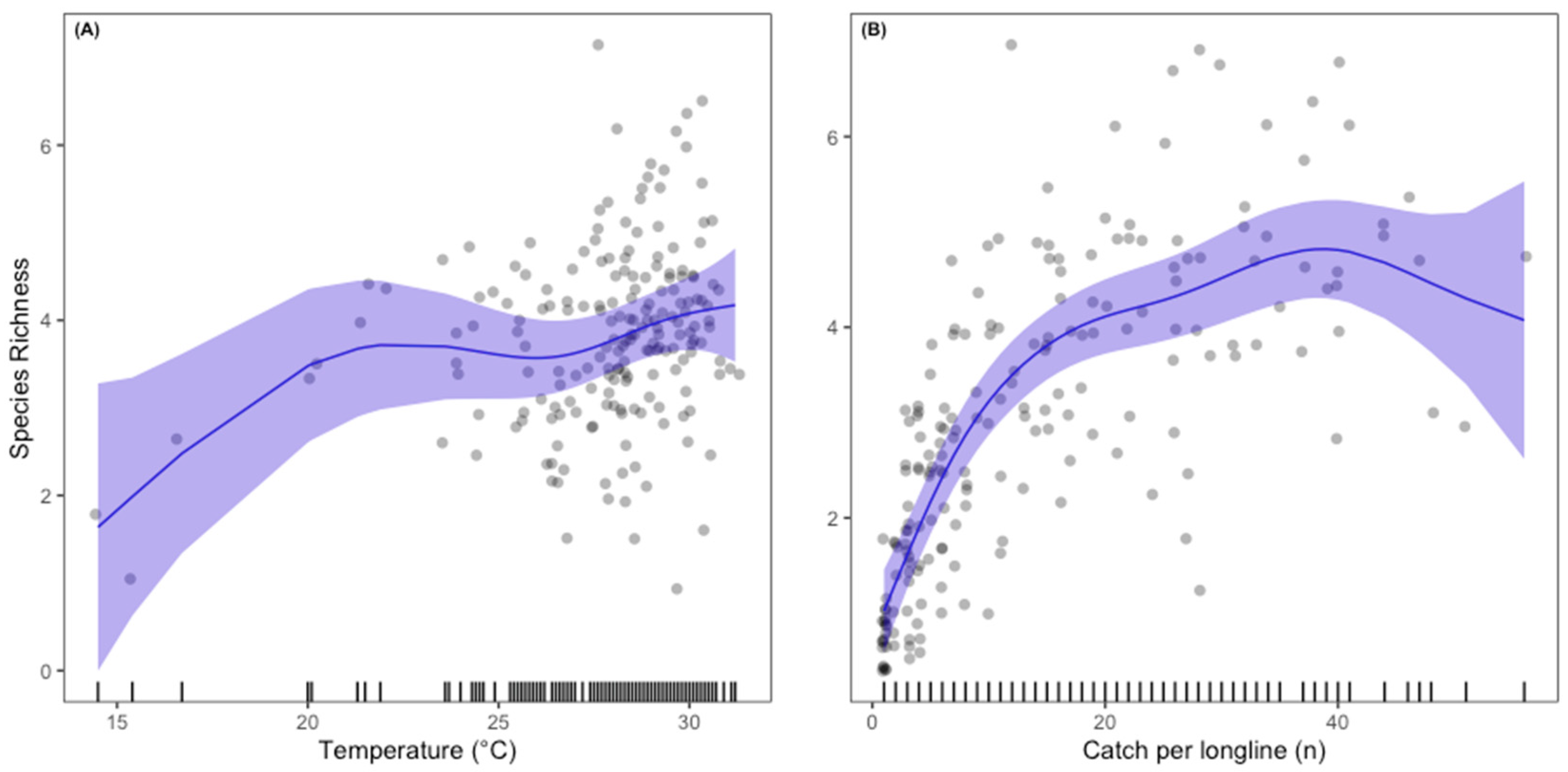
For species richness, model 4 with year, dissolved oxygen, temperature, and catch was selected as the final model (AICc = 569.0) (in Supplementary Materials), explaining 63.3% of the variance in species richness (adjusted R2 = 0.604). Smooth terms for temperature (edf = 3.537, F = 2.899, p-value = 0.018) and catch (edf = 4484, p-value < 0.0001) indicated significant non-linear effect on species richness (in Supplementary Materials). Species richness displayed a positive trend with temperature with observations aggregated between 27 and 30 °C, except for the slight decrease between 22 and 25 °C (Figure 2A). Species richness also displayed a positive trend with catch per longline (Figure 2B).
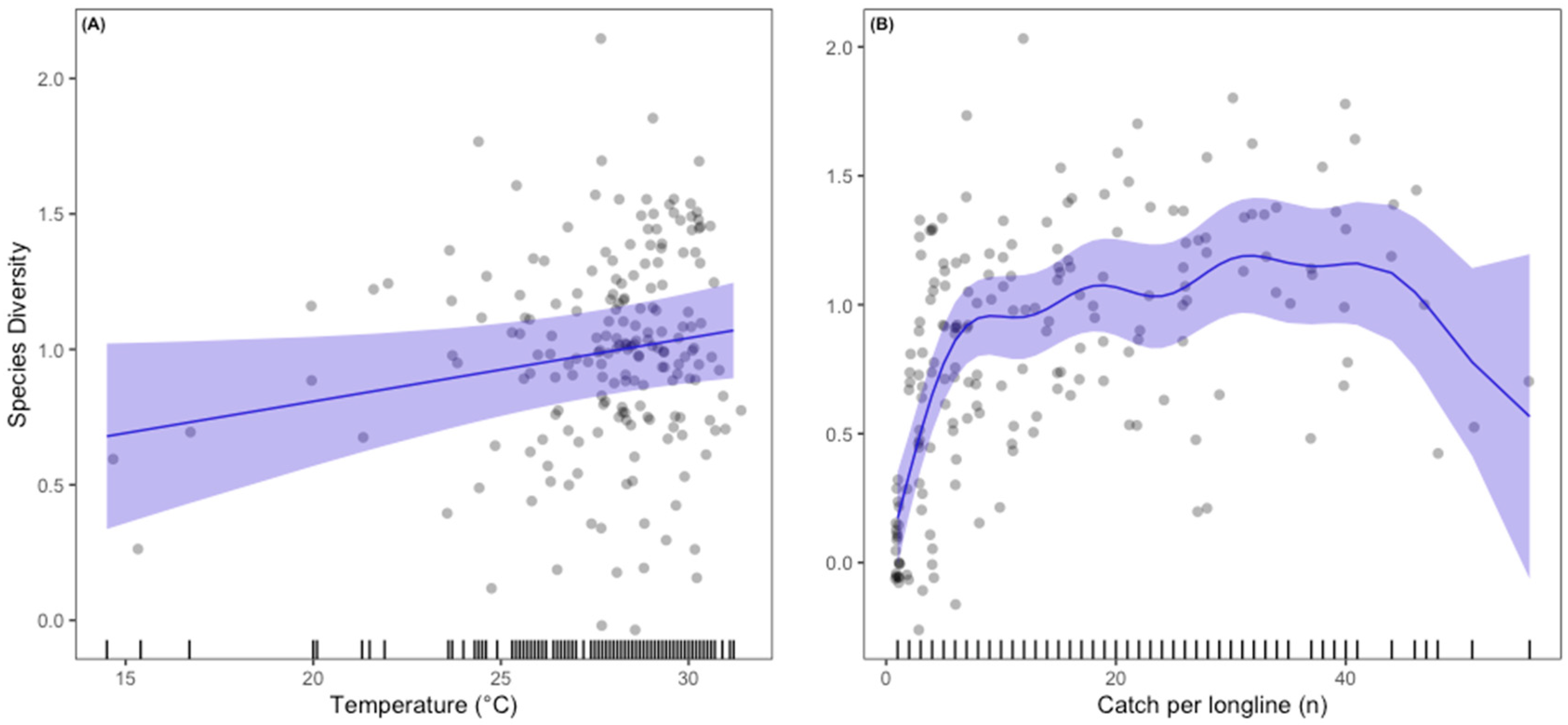
For species diversity, model 4 with salinity, dissolved oxygen, temperature, and catch was selected as the final model (AICc value = 172.6) (in Supplementary Materials), explaining 50% of the variance in species diversity (adjusted R2 = 0.451). The smooth terms for temperature (edf = 1, p-value = 0.0444) indicated significant linear effects with species diversity. The smooth term for catch (edf = 7.179, p-value < 0.0001) indicated significant non-linear effects on species diversity (in Supplementary Materials). Species diversity displayed a steady increasing trend with increasing temperature with an aggregation of observation between 25 and 28 °C (Figure 3A). Species diversity greatly increased with low catch per longline and fluctuated when 10–40 individuals were caught per longline (Figure 3B).
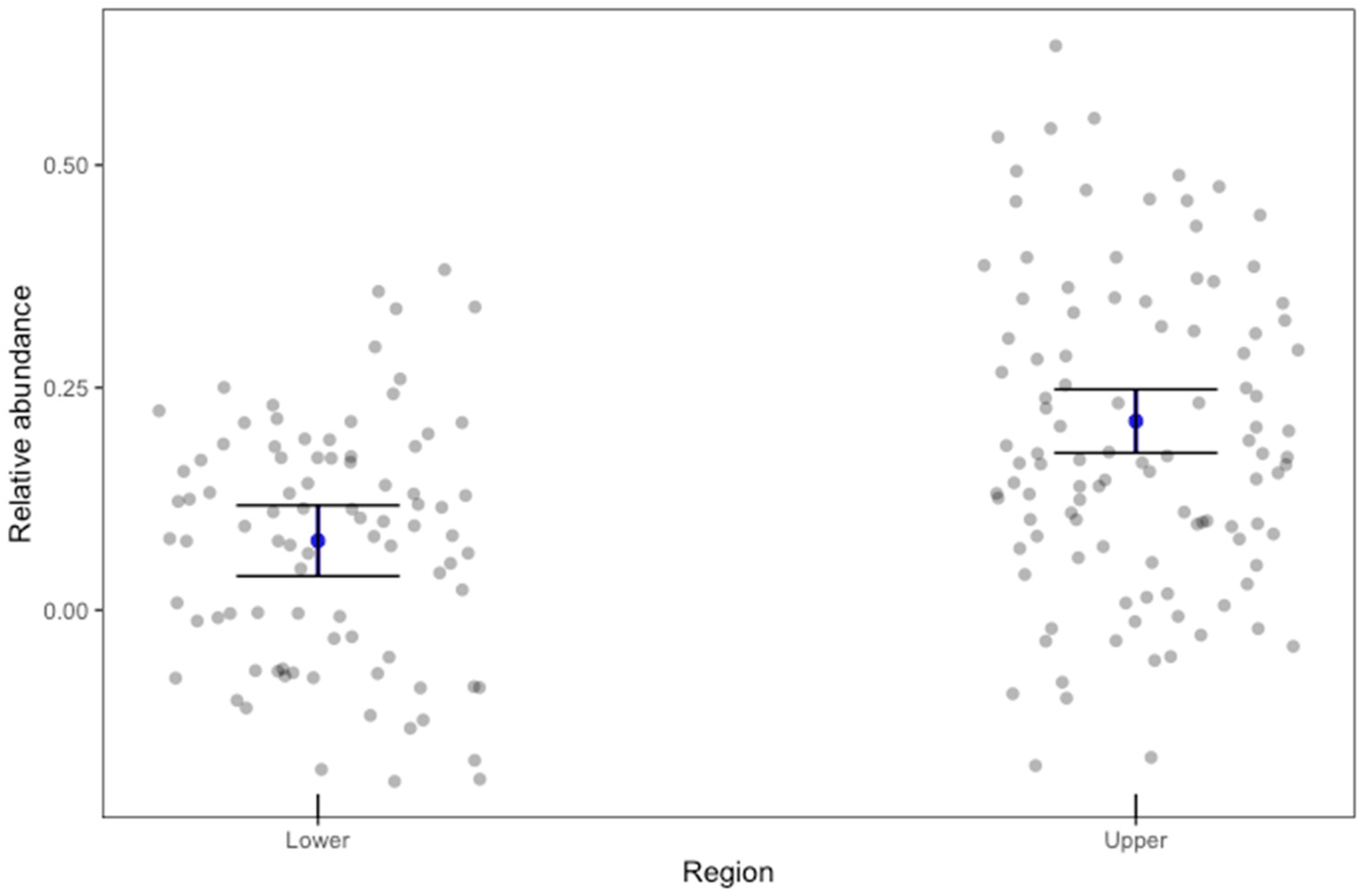
For relative abundance, model 1 with region, year, salinity, temperature, do, and depth was selected as the final model (AICc value = −302.3) (in Supplementary Materials), explaining 36.8% of the variance in relative abundance (adjusted R2 = 0.329). For region, p-value < 0.0001 indicated a significant effect on relative abundance (in Supplementary Materials). Relative abundance was significantly higher in the upper region than the lower region (Figure 4).

3.3. Predicted Presence Probability

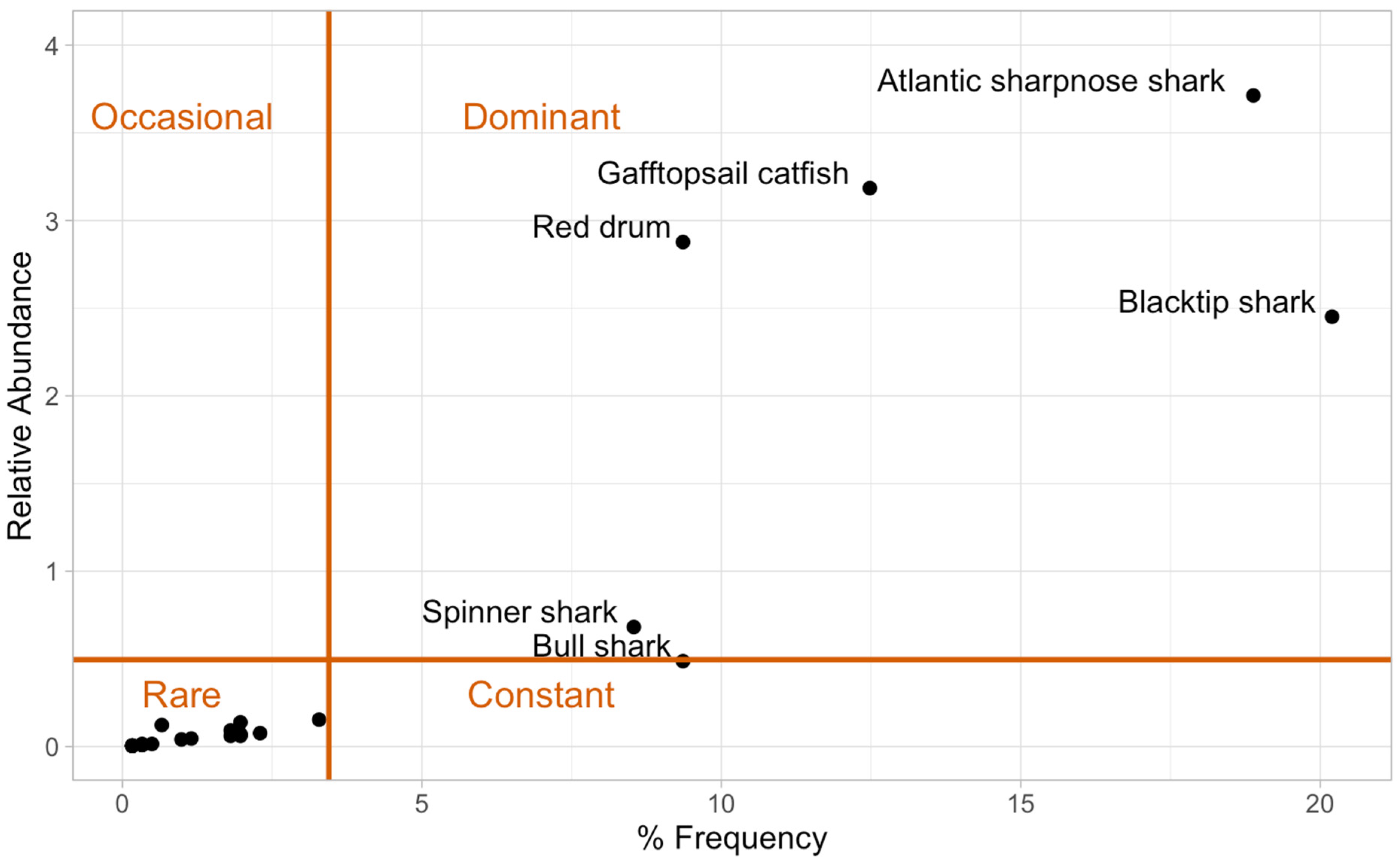
The Olmstead–Tukey corner test for association identified six dominant species: Atlantic sharpnose shark, gafftopsail catfish, red drum, blacktip shark, spinner shark, and bull shark (Figure 5). These species accounted for 93% of the total catch.
Region affected the presence probabilities of gafftopsail catfish, red drum, spinner shark, and bull sharks. The presence probabilities for these species were all significantly higher in the upper region than the lower region. Region also had interactive effects on other species. Atlantic sharpnose shark presence increased with depth in the upper region but decreased in the lower region. Salinity had a negative effect on blacktip shark presence in the lower region, but no effect in the upper region.
Results showed a significant temporal effect on three dominant species. Atlantic sharpnose sharks’ presence probability declined over time in varying DO conditions. Gafftopsail catfish probabilities also declined over the survey period in deeper water but increased in shallow water. Lastly, red drum probabilities increased in both high and low DO over time, but more with higher DO values.
Salinity did not directly affect any of the dominant species, but its interaction with other environmental drivers affected four of the six dominant species. Red drum presence probability declined with increasing salinity in all depths. For bull sharks, increasing salinity had opposing effects depending on water temperatures where high water temperatures displayed a stronger decline than cooler water temperatures. Increasing depths also negatively affected bull shark presence.
Water temperature directly influenced red drum presence probability, where presence declined as water temperature increased. However, temperature interactions with DO influenced the presence probabilities of three other dominant species. Presence probability of Atlantic sharpnose sharks increased with DO in high water temperatures and decreased in low water temperatures. Conversely, gafftopsail catfish and blacktip shark presence increased with DO in low water temperatures and decreased in high water temperatures. Significant effects were also observed with DO interacting with salinity. Presence probability of spinner sharks was negatively affected with increasing DO in high salinity conditions but showed slight increase in low salinity conditions. As a main variable, increasing DO had a positive effect on bull shark probabilities.

4. Discussion

In the present study, a multiyear (10-year period) assessment of bottom longline surveys of demersal fish assemblages was conducted along the nearshore Texas continental shelf within the GoM. Per our hypothesis, species richness, diversity, and abundance were significantly affected by water temperature and salinity, but also DO. When we further analyzed spatial, temporal, and environmental effects on the six dominant species, DO and temperature were the most influential environmental variables. Further analyses also supported a significant spatial effect on all six species.
Dominant species commonly occurring in the northwestern GoM include snappers (Lutjanidae), groupers (Serranidae), and drums (Sciaenidae) [13,16]. In this study, the dominance of red drum (Sciaenops ocellatus) coincides with findings in Murawski et al. (2018) [13]. However, no grouper or snapper species were caught during the survey, and a high percentage of species (76%) reported by Murawski et al. (2018) [13] differed from species caught for the present study. Differences between studies could be attributed to shallower survey depths in the present study (<23 m) compared to deeper survey depths in the previous study (>200 m). Differing assemblages could also be due to various habitat types within the GoM having unique fish assemblages [14,17,37]. These contradictions underpin the need for more continuous local or small-scale long-term monitoring programs to obtain a deeper understanding of the trends and patterns for fish communities throughout the GoM.
Temperature was one of the most influential environmental factors in this study, where a high density of observations for both species richness and diversity was seen between 25 and 28 °C, which is a common variable in studies as temperature can have significant effects on fish physiology and ecology, such as growth, metabolism, movement, and reproduction [9,38,39]. Catch was another influential factor in this study. The previous literature states the importance of capturing the effect of abundance and sampling efforts on species richness and diversity using rarefaction curves [29,30]. We did not use rarefaction curves, but we did observe a similar trendline in our results for species richness and species diversity which coincides with the previous literature stating the importance of including catch rates as a function of the measurement for species richness and diversity. We did observe a significant spatial effect on relative abundance, which could be due to significant spatial effects on dominant species of the survey.
Each of the six dominant species displayed a significant spatial effect. Higher presence probability in the upper region may be due to prey availability and distribution [15,40]. For example, blue crabs (Callinectes sapidus) are an important component of gafftopsail catfish and red drum diets. Salt marshes along the upper Texas and Louisiana coast—and the upper region of this study—are expected to be of great value to blue crabs as a nursery [41,42], which provides a potential explanation for greater presence probability of red drum and gafftopsail catfish in the upper region. Red drum and gafftopsail catfish are prey items for bull sharks and spinner sharks [43,44,45] whose presence probability was high in the upper region of the study. Researchers have also found sciaenids to be an abundant prey group in blacktip and Atlantic sharpnose sharks’ diets, whose presence probability was significantly influenced by region as an interactive term with depth. Therefore, prey availability and distribution could have caused the significant effect observed on presence probability paired with significant environmental drivers.
In addition to significant spatial effects on dominant species presence, we found significant environmental drivers to be important. Contrary to our hypothesis of a significant salinity and temperature effect on fish assemblages, as those are the two most common variables considered as environmental drivers, we found temperature and DO to be more common drivers of presence probability either as a main variable or as an interaction term. Though, we did not find common patterns in DO and temperature trends across the six species, which could suggest strong preferences of environmental conditions, but we would need the associated habitat data to make these inferences. Though DO is a crucial factor for aerobic fish species survival, it is not a commonly considered driver for parameters such as abundance and distribution. The effects of DO on fish include a stunt in growth, delayed spawning, and decreased reproduction rates [46]. Demersal fishes have been cited to be the most affected by low DO conditions, as low DO is limited to bottom waters [47]. Few studies have attempted to establish a pattern on how DO affects species abundance, but no common pattern has emerged other than species migrating to oxygenated areas [48]. For example, researchers suggested a relationship between DO and species size, citing that larger species will have higher survival rates due to more gill surface area [49,50]. However, a review of such studies found opposing results where both large and small species survived regardless of body size [51]. Nonetheless, our results introduce DO and temperature as a driving factor in the study as opposed to salinity and temperature, which are more commonly considered variables.

5. Conclusions

This study reports results from a long-term monitoring dataset of demersal fishes along the continental shelf of the Texas region in the GoM. Findings provide a baseline evaluation of environmental conditions and biology, while also highlighting the importance and contributions of continued monitoring and deeper understanding of multiple factors that influence the distribution of demersal fish assemblages in the Texas region of the GoM. This research focused exclusively on environmental drivers that impacted the distribution of studied species; however, further ecological assessments that include additional natural (e.g., chlorophyll, season, time of day, habitat type, and turbidity) and anthropogenic factors (e.g., nutrient levels) could provide stronger inferences on the distribution patterns of demersal fishes in highly dynamic marine ecosystems, including the GoM. Methodological limitations such as gear selectivity may have also influenced study results. Although bottom longline gear is common and efficient for surveys, longline gear can be species and size selective for larger individuals as not all fish species and sizes are susceptible to longline gear [23,52]. Conducting surveys of this caliber can also present logistical limitations such as lack of personnel for a full fishing crew, lack of resources (e.g., a full equipped and capable boat), as well as funding complications for gear purchase. Future studies could benefit from the addition of other fishing techniques such as trawls and gillnets for a more conclusive look at the fish assemblage patterns in the GoM.

Supplementary Materials

The following supporting information can be downloaded at: https://www.mdpi.com/article/10.3390/fishes10120632/s1, The supplementary materials contain tables and figures from the model selection process for species richness, species diversity, relative abundance and presence probabilities of the six (6) dominant species of the survey. The supplementary materials also contain figures of predicted presence probabilities for the six (6) dominant species of the survey.

Author Contributions

Conceptualization, E.M.J. and R.J.D.W.; methodology, E.M.J., F.M.-A., P.S.D.-S., A.G.-H., C.L. and R.J.D.W.; software, E.M.J., P.S.D.-S. and A.G.-H.; validation, E.M.J., F.M.-A., A.G.-H. and C.L.; formal analysis, E.M.J., P.S.D.-S. and A.G.-H.; investigation, E.M.J. and R.J.D.W.; resources, F.M.-A.; data curation, E.M.J., F.M.-A., P.S.D.-S. and R.J.D.W.; writing—original draft preparation, E.M.J. and R.J.D.W.; writing—review and editing, E.M.J., F.M.-A., P.S.D.-S., A.G.-H., C.L. and R.J.D.W.; visualization, E.M.J.; supervision, R.J.D.W.; project administration, E.M.J., F.M.-A. and R.J.D.W.; funding acquisition, F.M.-A. All authors have read and agreed to the published version of the manuscript.

Funding

This research was funded by Southeast Area Monitoring and Assessment Program (SEAMAP) and Texas Parks & Wildlife Department, permit number SER-2009-07541.

Institutional Review Board Statement

Not applicable.

Informed Consent Statement

Not applicable.

Data Availability Statement

Data are available upon request to the Texas Parks & Wildlife Department.

Acknowledgments

We thank the members of the Shark Biology and Fisheries Science Lab at TAMUG for assistance with the project. We also thank Blair Sterba-Boatwright for developing source codes utilized in the data analysis of this study.

Conflicts of Interest

The authors declare no conflicts of interest.

Abbreviations

The following abbreviations are used in this manuscript:
GoMGulf of Mexico
TPWDTexas Parks & Wildlife Department
SEAMAPSoutheast Area Monitoring and Assessment Program
NMFSNational Marine Fisheries Service
CPUECatch Per Unit Effort
DODissolved Oxygen
AICcCorrected Akaike Information Criterion
edfEffective Degrees of Freedom
GAMsGeneralizes Additive Models

References

  1. Nogueira, A.; Gonzalez-Troncoso, D.; Tolimieri, N. Changes and Trends in the Overexploited Fish Assemblages of Two Fishing Grounds of the Northwest Atlantic. ICES J. Mar. Sci. 2015, 73, 345–358. [Google Scholar] [CrossRef]
  2. Steichen, J.; Quigg, A. Fish Species as Indicators of Freshwater Inflow within a Subtropical Estuary in the Gulf of Mexico. Ecol. Indic. 2018, 85, 180–189. [Google Scholar] [CrossRef]
  3. Jones, H.; Johnson, K.; Kelly, M. Synergistic Effects of Temperature and Salinity on the Gene Expression and Physiology of Crassostrea virginica. Integr. Comp. Biol. 2019, 59, 306–319. [Google Scholar] [CrossRef] [PubMed]
  4. Vergés, A.; Steinberg, P.D.; Hay, M.E.; Poore, A.G.B.; Campbell, A.H.; Ballesteros, E.; Heck, K.L.; Booth, D.J.; Coleman, M.A.; Feary, D.A.; et al. The Tropicalization of Temperate Marine Ecosystems: Climate-Mediated Changes in Herbivory and Community Phase Shifts. Proc. R. Soc. B Biol. Sci. 2014, 281, 20140846. [Google Scholar] [CrossRef] [PubMed]
  5. Zenteno-Savín, T. Diurnal and Seasonal Hsp70 Gene Expression in a Cryptic Reef Fish, the Bluebanded Goby Lythrypnus dalli (Gilbert 1890). Biotecnia 2021, 23, 81–88. [Google Scholar] [CrossRef]
  6. Radfar, S.; Moftakhari, H.; Moradkhani, H. Rapid Intensification of Tropical Cyclones in the Gulf of Mexico Is More Likely during Marine Heatwaves. Commun. Earth Environ. 2024, 5, 421. [Google Scholar] [CrossRef]
  7. Wang, Z.; Boyer, T.; Reagan, J.; Hogan, P. Upper-Oceanic Warming in the Gulf of Mexico between 1950 and 2020. J. Clim. 2023, 36, 2721–2734. [Google Scholar] [CrossRef]
  8. Gilford, D.M.; Giguere, J.; Pershing, A.J. Human-Caused Ocean Warming Has Intensified Recent Hurricanes. Environ. Res. Clim. 2024, 3, 045019. [Google Scholar] [CrossRef]
  9. Fujiwara, M.; Martinez-Andrade, F.; Wells, R.J.D.; Fisher, M.; Pawluk, M.; Livernois, M.C. Climate-Related Factors Cause Changes in the Diversity of Fish and Invertebrates in Subtropical Coast of the Gulf of Mexico. Commun. Biol. 2019, 2, 403. [Google Scholar] [CrossRef]
  10. Rabalais, N.N.; Turner, R.E. Gulf of Mexico Hypoxia: Past, Present, and Future. Limnol. Ocean. Bull. 2019, 28, 117–124. [Google Scholar] [CrossRef]
  11. Lohner, T.; Dixon, D. The Value of Long-Term Environmental Monitoring Programs: An Ohio River Case Study. Environ. Monit. Assess. 2013, 185, 9385–9396. [Google Scholar] [CrossRef]
  12. Rabalais, N.; Turner, R.E.; Scavia, D. Beyond Science into Policy: Gulf of Mexico Hypoxia and the Mississippi River: Nutrient Policy Development for the Mississippi River Watershed Reflects the Accumulated Scientific Evidence That the Increase in Nitrogen Loading Is the Primary Factor in the Worsening of Hypoxia in the Northern Gulf of Mexico. BioScience 2002, 52, 129–142. [Google Scholar] [CrossRef]
  13. Murawski, S.A.; Peebles, E.B.; Gracia, A.; Tunnell, J.W.; Armenteros, M. Comparative Abundance, Species Composition, and Demographics of Continental Shelf Fish Assemblages throughout the Gulf of Mexico. Mar. Coast. Fish. 2018, 10, 325–346. [Google Scholar] [CrossRef]
  14. Wells, R.J.D.; Harper, J.O.; Rooker, J.R.; Landry, A.M., Jr.; Dellapenna, T.M. Fish Assemblage Structure on a Drowned Barrier Island in the Northwestern Gulf of Mexico. Hydrobiologia 2009, 625, 207–221. [Google Scholar] [CrossRef]
  15. Monk, M.; Powers, J.; Brooks, E. Spatial Patterns in Species Assemblages Associated with the Northwestern Gulf of Mexico Shrimp Trawl Fishery. Mar. Ecol. Prog. Ser. 2015, 519, 1–12. [Google Scholar] [CrossRef]
  16. Ward, C.; Tunnell, J., Jr. Habitats and Biota of the Gulf of Mexico: An Overview. In Habitats and Biota of the Gulf of Mexico: Before the Deepwater Horizon Oil Spill; Springer: New York, NY, USA, 2017. [Google Scholar]
  17. Ajemian, M.; Wetz, J.; Shipley-Lozano, B.; Shively, J.D.; Stunz, G. An Analysis of Artificial Reef Fish Community Structure along the Northwestern Gulf of Mexico Shelf: Potential Impacts of “Rigs-to-Reefs” Programs. PLoS ONE 2015, 10, e0126354. [Google Scholar] [CrossRef]
  18. Mendelssohn, I.; Byrnes, M.; Kneib, R.; Vittor, B. Coastal Habitats of the Gulf of Mexico. In Habitats and Biota of the Gulf of Mexico: Before the Deepwater Horizon Oil Spill; Springer: New York, NY, USA, 2017; pp. 359–640. [Google Scholar]
  19. Chu, J.W.; Tunnicliffe, V. Oxygen Limitations on Marine Animal Distributions and the Collapse of Epibenthic Community Structure during Shoaling Hypoxia. Glob. Change Biol. 2015, 21, 2989–3004. [Google Scholar] [CrossRef]
  20. Heupel, M.; Yeiser, B.; Collins, A.; Ortega, L.; Cimpfendorfer, C. Long-Term Presence and Movement Patterns of Juvenile Bull Sharks, Carcharhinus leucas, in an Estuarine River System. Mar. Freshw. Res. 2010, 61, 1–10. [Google Scholar] [CrossRef]
  21. Hendon, J.M.; Hoffmayer, E.R.; Pollack, A.G.; Mareska, J.; Martinez-Andrade, F.; Rester, J.; Switzer, T.S.; Zuckerman, Z.C. Impacts of Survey Design on a Gulf of Mexico Bottom Longline Survey and the Transition to a Unified, Stratified - Random Design. Front. Mar. Sci. 2025, 11, 1426756. [Google Scholar] [CrossRef]
  22. Bugica, K.; Sterba-Boatwright, B.; Wetz, M.S. Water Quality Trends in Texas Estuaries. Mar. Pollut. Bull. 2020, 152, 110903. [Google Scholar] [CrossRef]
  23. Menezes, G.; Sigler, M.F. Longlines. In Biological Sampling in the Deep Sea; Clark, M.R., Consalvey, M., Rowden, A.A., Eds.; Wiley Blackwell: Hoboken, NJ, USA, 2016; pp. 159–183. [Google Scholar]
  24. Drymon, J.M.; Carassou, L.; Powers, S.P.; Grace, M.; Dindo, J.; Dzwonkowski, B. Multiscale Analysis of Factors That Affect the Distribution of Sharks throughout the Northern Gulf of Mexico. Fish. Bull. 2013, 111, 370–380. [Google Scholar] [CrossRef]
  25. Su, Q. A Relationship between Species Richness and Evenness That Depends on Specific Relative Abundance Distribution. PeerJ 2018, 6, e4951. [Google Scholar] [CrossRef] [PubMed]
  26. Oksanen, J.; Simpson, G.L.; Blanchet, F.G.; Kindt, R.; Legendre, P.; Minchin, P.R.; O’Hara, R.B.; Solymos, P.; Stevens, M.H.H.; Szoecs, E.; et al. Vegan: Community Ecology Package 2001, 2.7-2. Available online: https://cran.r-project.org/web/packages/vegan/index.html (accessed on 3 October 2025).
  27. Shannon, C.E. A Mathematical Theory of Communication. Bell Syst. Tech. J. 1948, 27, 379–423. [Google Scholar] [CrossRef]
  28. Allen, M.L.; Roberts, N.M.; Bauder, J.M. Relationships of Catch-per-Unit-Effort Metrics with Abundance Vary Depending on Sampling Method and Population Trajectory. PLoS ONE 2020, 15, e0233444. [Google Scholar] [CrossRef]
  29. Gotelli, N.J.; Colwell, R.K. Quantifying Biodiversity: Procedures and Pitfalls in the Measurement and Comparison of Species Richness. Ecol. Lett. 2001, 4, 379–391. [Google Scholar] [CrossRef]
  30. Gwinn, D.C.; Allen, M.S.; Bonvechio, K.I.; Hoyer, M.V.; Beesley, L.S. Evaluating Estimators of Species Richness: The Importance of Considering Statistical Error Rates. Methods Ecol. Evol. 2016, 7, 294–302. [Google Scholar] [CrossRef]
  31. Wood, S.N. Fast Stable Restricted Maximum Likelihood and Marginal Likelihood Estimation of Semiparametric Generalized Linear Models. J. R. Stat. Soc. Ser. B Stat. Methodol. 2011, 73, 3–36. [Google Scholar] [CrossRef]
  32. Zuur, A.; Ieno, E.; Walker, N.; Saveliev, A.; Smith, G. Mixed Effects Models and Extensions in Ecology with R; Springer: New York, NY, USA, 2009; ISBN 978-0-387-87457-9. [Google Scholar]
  33. Anderson, D.; Burnham, K. Model Selection and Multimodel Inference: A Practical Information-Theoretic Approach; Springer: New York, NY, USA, 2002; ISBN 978-0-387-95364-9. [Google Scholar]
  34. Olmstead, P.S.; Tukey, J.W. A Corner Test for Association. Ann. Math. Stat. 1947, 18, 495–513. [Google Scholar] [CrossRef]
  35. Livernois, M.C.; Power, S.; Albins, M. Habitat Associations and Co-Occurrence Patterns of Two Estuarine-Dependent Predatory Fishes. Mar. Coast. Fish. 2020, 12, 64–77. [Google Scholar] [CrossRef]
  36. McCabe, C.; Halvorson, M.; King, K.; Cao, X.; Kim, D. Interpreting Interaction Effects in Generalized Linear Models of Nonlinear Probabilities and Counts. Multivar. Behav. Res. 2021, 57, 243–263. [Google Scholar] [CrossRef]
  37. Rezneat, D. Regional Environments and Topographic Features. In The American Sea: A Natural History of the Gulf of Mexico; Texas A&M University Press: College Station, TX, USA, 2015; pp. 38–59. [Google Scholar]
  38. Mitchell, A.; Hayes, C.; Booth, D.J.; Nagelkerken, I. Future Shock: Ocean Acidification and Seasonal Water Temperatures Alter the Physiology of Competing Temperate and Coral Reef Fishes. Sci. Total Environ. 2023, 883, 163684. [Google Scholar] [CrossRef]
  39. Lindmark, M.; Audzijonyte, A.; Blanchard, J.L.; Gårdmark, A. Temperature Impacts on Fish Physiology and Resource Abundance Lead to Faster Growth but Smaller Fish Sizes and Yields under Warming. Glob. Change Biol. 2022, 28, 6239–6253. [Google Scholar] [CrossRef]
  40. Scharf, F.S.; Schlight, K.K. Feeding Habits of Red Drum (Sciaenops ocellatus) in Galveston Bay, Texas: Seasonal Diet Variation and Predator-Prey Size Relationships. Estuaries 2000, 23, 128. [Google Scholar] [CrossRef]
  41. Thomas, J.L.; Zimmerman, R.J.; Minello, T.J. Abundance patterns of juvenile blue crabs (Callinectes sapidus) in nursery habitats of two Texas bays. Bull. Mar. Sci. 1990, 46, 115–125. [Google Scholar]
  42. Marchessaux, G.; Gjoni, V.; Sarà, G. Environmental Drivers of Size-Based Population Structure, Sexual Maturity and Fecundity: A Study of the Invasive Blue Crab Callinectes sapidus (Rathbun, 1896) in the Mediterranean Sea. PLoS ONE 2023, 18, e0289611. [Google Scholar] [CrossRef] [PubMed]
  43. Cottrant, E.; Matich, P.; Fisher, M. Boosted Regression Tree Models Predict the Diets of Juvenile Bull Sharks in a Subtropical Estuary. Mar. Ecol. Prog. Ser. 2021, 659, 127–141. [Google Scholar] [CrossRef]
  44. TinHan, T.C.; Wells, R.J.D. Spatial and Ontogenetic Patterns in the Trophic Ecology of Juvenile Bull Sharks (Carcharhinus leucas) From the Northwest Gulf of Mexico. Front. Mar. Sci. 2021, 8, 664316. [Google Scholar] [CrossRef]
  45. Osmany, H.B.; Moazzam, M. Species composition, commercial landings, distribution and some aspects of biology of shark (Class Pisces) of Pakistan: Large demersal sharks. Int. J. Biol. Biotechnol. 2022, 19, 89–111. [Google Scholar]
  46. Kim, H.; Franco, A.C.; Sumaila, U.R. A Selected Review of Impacts of Ocean Deoxygenation on Fish and Fisheries. Fishes 2023, 8, 316. [Google Scholar] [CrossRef]
  47. Nodo, P.; Childs, A.-R.; Pattrick, P.; Lemley, D.A.; James, N.C. Response of Demersal Fishes to Low Dissolved Oxygen Events in Two Eutrophic Estuaries. Estuar. Coast. Shelf Sci. 2023, 293, 108514. [Google Scholar] [CrossRef]
  48. Buchheister, A.; Bonzek, C.; Gartland, J.; Latour, R. Patterns and Drivers of the Demersal Fish Community of Chesapeake Bay. Mar. Ecol. Prog. Ser. 2013, 481, 161–180. [Google Scholar] [CrossRef]
  49. Friedman, J.R.; Condon, N.E.; Drazen, J.C. Gill Surface Area and Metabolic Enzyme Activities of Demersal Fishes Associated with the Oxygen Minimum Zone off California. Limnol. Oceanogr. 2012, 57, 1701–1710. [Google Scholar] [CrossRef]
  50. Robb, T.; Abrahams, M.V. Variation in Tolerance to Hypoxia in a Predator and Prey Species: An Ecological Advantage of Being Small? J. Fish Biol. 2003, 62, 1067–1081. [Google Scholar] [CrossRef]
  51. Nilsson, G.E.; Östlund-Nilsson, S. Does Size Matter for Hypoxia Tolerance in Fish? Biol. Rev. 2008, 83, 173–189. [Google Scholar] [CrossRef] [PubMed]
  52. Hubert, W.; Pope, K.; Dettmers, J. Passive Capture Techniques. In Fisheries Techniques; Zale, A.V., Parrish, D.L., Sutton, T.M., Eds.; American Fisheries Society: Bethesda, MD, USA, 2012; pp. 223–265. [Google Scholar]
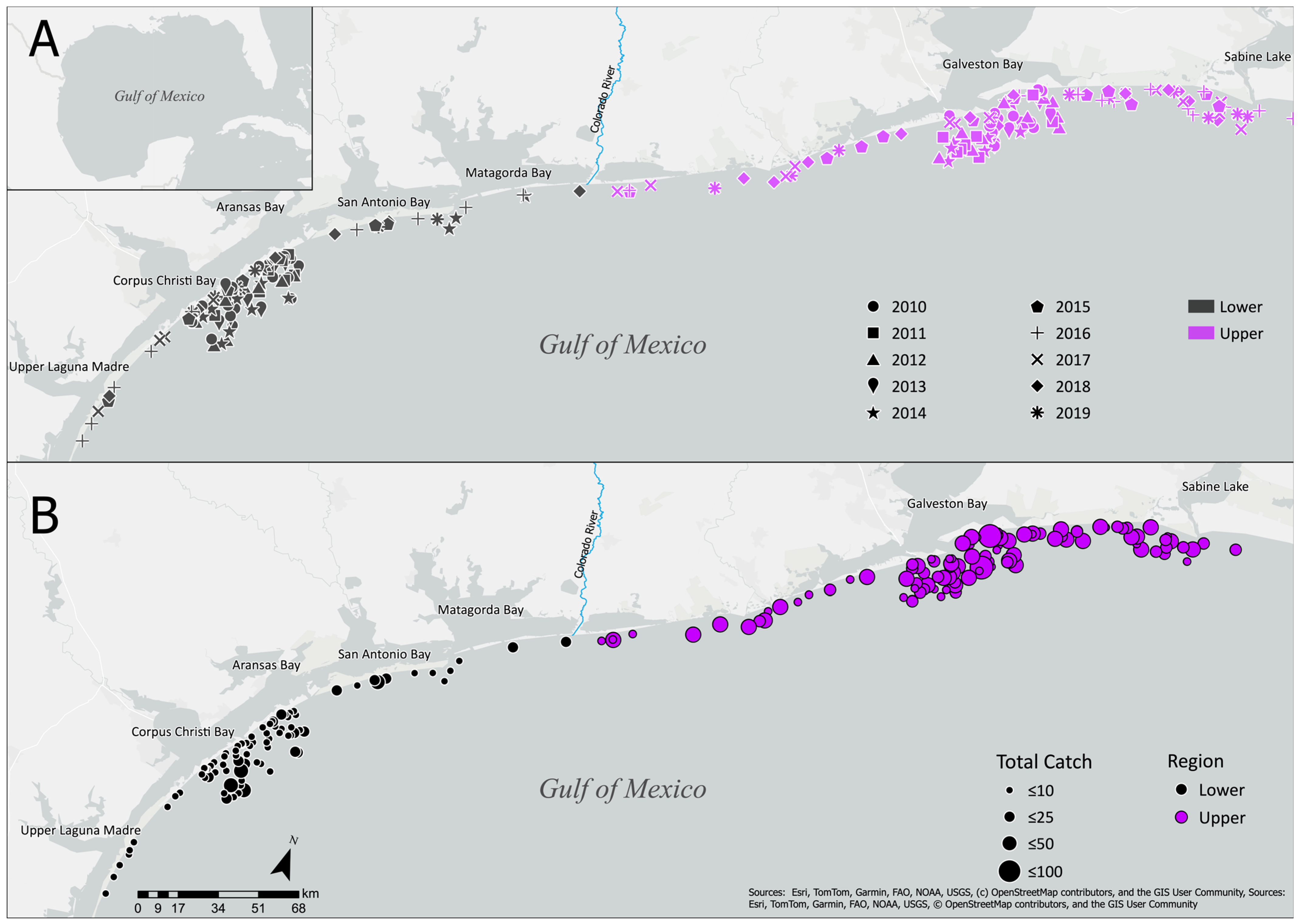
Figure 1. Sampling location with maps showing (A) the distribution of longlines per year and (B) the total catch per longline using graduate symbols. In map A, each symbol represents a survey year. In both maps, purple represents the upper region and black represents the lower region.
Fishes 10 00632 g001
Figure 2. Partial effect of temperature (A) and catch per longline (B) on species richness. Points within the graph represent residual from model. Polygons indicate 95% confidence intervals.
Fishes 10 00632 g002
Figure 3. Partial effect of temperature (A) and catch per longline (B) on species diversity. Points within the graph represent residuals from model. Polygons indicate 95% confidence intervals.
Fishes 10 00632 g003
Figure 4. Partial effect of region on relative abundance. Points within the graph represent residuals from model. Polygons and error bars indicate 95% confidence intervals.
Fishes 10 00632 g004
Figure 5. Olmstead–Tukey corner test of association for species caught during the longline survey (2010–2019) along the Texas coast of the Gulf of Mexico. Black points indicate individual species with dominant species labeled. Orange axes indicate mean values of relative abundance (y-axis) and frequency of occurrence (x-axis).
Fishes 10 00632 g005
Table 1. Summary of species caught during bottom longline survey along the Texas region of the Gulf of Mexico, including species’ common and scientific names, total catch (n), descriptive statistics of lengths for each species where applicable and species frequency (Freq). TL represents total length, DW represents disk width, SD represents standard deviation.
Common NameScientific NamenTL/DW (mm)Freq
MeanSDMinMax
Atlantic Sharpnose SharkRhizoprionodon terraenovae724891134.03351136115
Gafftopsail CatfishBagre marinus62151455.819588076
Red DrumSciaenops ocellatus56193560.7745187657
Blacktip SharkCarcharhinus limbatus4781282268.34391923123
Spinner SharkCarcharhinus brevipinna1331118345.2645204052
Bull SharkCarcharhinus leucas951705330.5886274357
Finetooth SharkCarcharhinus isodon301080290.3650145320
Blacknose SharkCarcharhinus acronotus27109853.8944117312
Sandbar SharkCarcharhinus plumbeus241104174.688115754
Black DrumPogonias cromis1882976.963899311
Scalloped Hammerhead Sphyrna lewini151563645.6543247414
Southern StingrayHypanus americanus141053221.0775139412
Great HammerheadSphyrna mokarran122147275.31700268911
Hardhead CatfishAriopsis felis1235029.929440612
BonnetheadSphyrna tiburo9971149.671111827
Roughtail StingrayBathytoshia centroura81020246.578715346
SharksuckerEcheneis naucrates31407.61321472
Tiger SharkGaleocerdo cuvier32041236.2187422083
Atlantic StingrayHypanus sabinus2686178.95598122
Bluntnose StingrayHypanus say2106389.1100011262
Lemon SharkNegaprion brevirostris22558345.8231328022
Spanish MackerelScomberomorus maculatus258654.55476242
Crevalle JackCaranx hippos1972 1
DolphinfishCoryphaena hippurus1828 1
Snapper EelEchiophis punctifer1733 1
Shrimp EelOphichthus gomesi1633 1
Atlantic Thread HerringOpisthonema oglinum1215 1
CobiaRachycentron canadum11184 1
Cownose RayRhinoptera bonasus1880 1
Total292802
Disclaimer/Publisher’s Note: The statements, opinions and data contained in all publications are solely those of the individual author(s) and contributor(s) and not of MDPI and/or the editor(s). MDPI and/or the editor(s) disclaim responsibility for any injury to people or property resulting from any ideas, methods, instructions or products referred to in the content.