
Systematic Approach for the Test Data Generation and Validation of ISC/ESC Detection Methods


Abstract
1. Introduction
- Reduction in heat influx from adjacent TRs to slow down or rather prevent TP in accordance with the US Vehicle Battery Safety Roadmap Guidance, which states that TP must not be initiated [17] if a never fully excluded cell-level TR occurs [18]. Prevention by smart module design [19,20], active or passive cooling strategies [21,22] and/or thermal isolation [23].
- Detection of battery faults and abnormal conditions for countermeasures, warning and evacuation before a hazardous situation develops. Here, the Global Technical Regulation on Electrical Vehicle Safety (GTR-EVS) specifies at least 5 or enough time for egress [24].
- Extensive literature review of disturbances on the measurement signal and their magnitudes;
- Summary of common qualitative and quantitative evaluation criteria;
- Generation of test data with stochastic disturbances and variations with consideration of both fault-free and fault-containing samples with the scope of ISC and ESC;
- Example comparison based on binary classifiers and identification of optimum parameter combinations.
2. State of the Art
- Complexity or difficulty of the application, e.g.,
- -
- -
- Large fault model parameter sets [30];
- -
- -
- -
- -
- Simplifications and assumptions concerning:
2.1. Measurement Uncertainty
2.2. Cell-to-Cell Variations
- Orientation at statistical founded experimentally determined variations;
- Assessment of the worst case boundaries.

| Author et al. | Year | Cell | /Ah | Source | ||
|---|---|---|---|---|---|---|
| Dey | 2016 | 5, 10 and 15 | [77] | |||
| Chang | 2019 | 18650 cell | 2 | 10, 20 and 40 | 20 | [130] |
| Chen | 2019 | A123 ANR26650-M1A | 2300 | ±3 | [30] | |
| Dubarry | 2019 | 0.0, 3.75, 7.5, 12.5 and 15 | 0.0, 1.25, 2.5, 3.75 and 5 | [131] | ||
| Zhang | 2019 | −5, −3, 2 and 5 | −5, −3, 2 and 5 | [68] | ||
| Schmid | 2021 | Samsung INR18650-25R | 2500 | +10 | [42] | |
| Song | 2021 | 60 | 0, 1.5 and 2.8 | [132] |
Voltage Offset
2.3. Evaluation Aspects
| True positive | True negative | |||
| False positive | False negative |
3. Material and Methods
3.1. Reference Cell
3.2. Model
- Parameterization is doable by standard electrochemical tests;
- Implementation of parameter distribution is simplified;
- Fault representation (see below) is well-defined;
- Simulation time is fast.
3.2.1. ISC/ESC-Fault Representation
3.2.2. Randomness and Variation
Measurement Uncertainty
Cell-to-Cell Variation
3.2.3. Parameterization
3.3. Simulation Cases
- The fault chance is 80%;
- Only one cell fault per time;
- Only one fault event per simulation run.
3.4. Fault Detection Methods
- Generate many samples without presence of a fault.
- Calculate the fault signals for the detection method for each sample.
- Determine the maximal fault signal value for each sample.
- Define the threshold as .
- If the fault signal is greater than a fault will be assumed.
3.4.1. Deviation from Mean
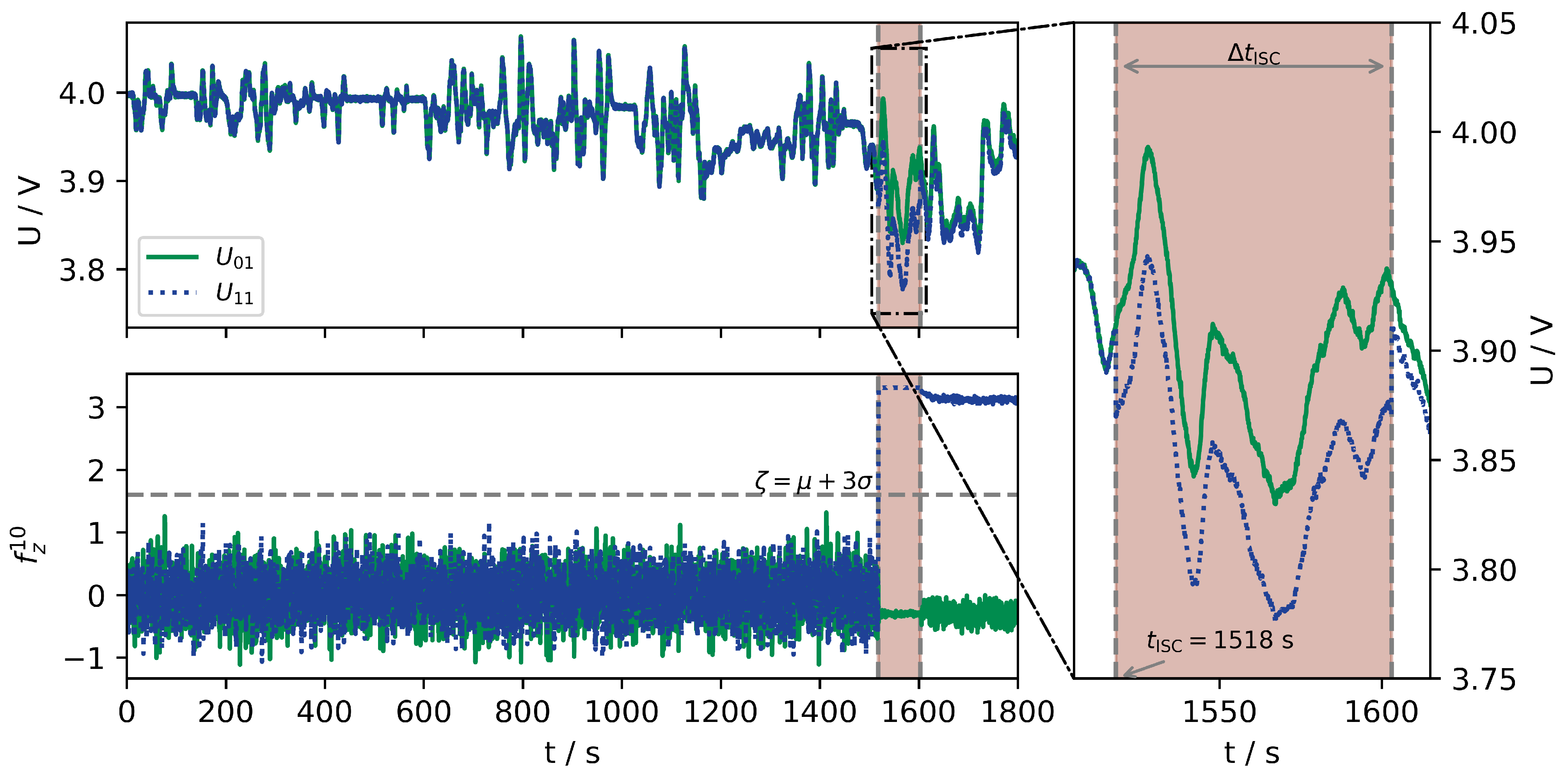
3.4.2. z-Score
4. Results and Discussion
4.1. Number of Simulations
4.2. Distribution of Fault Feature
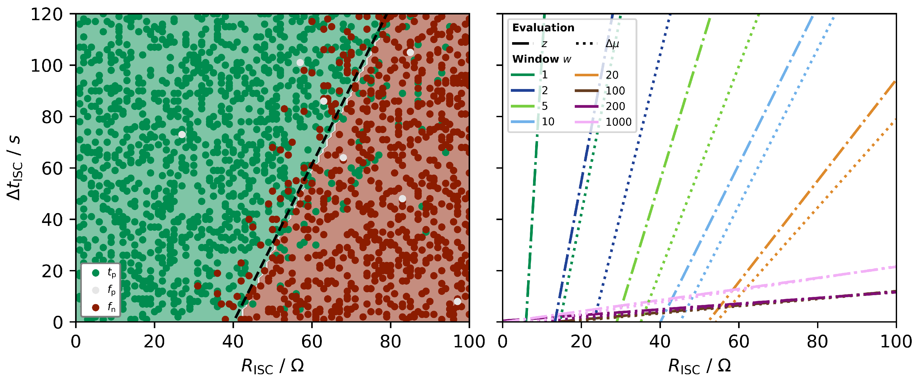
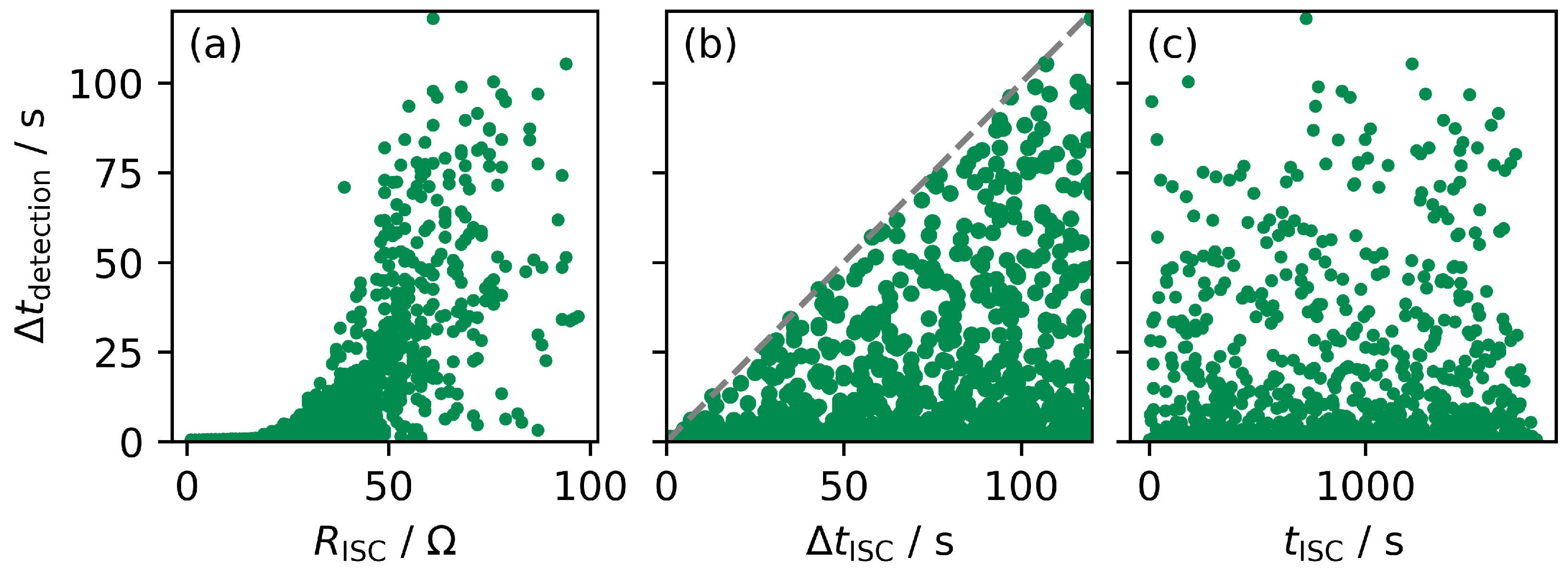
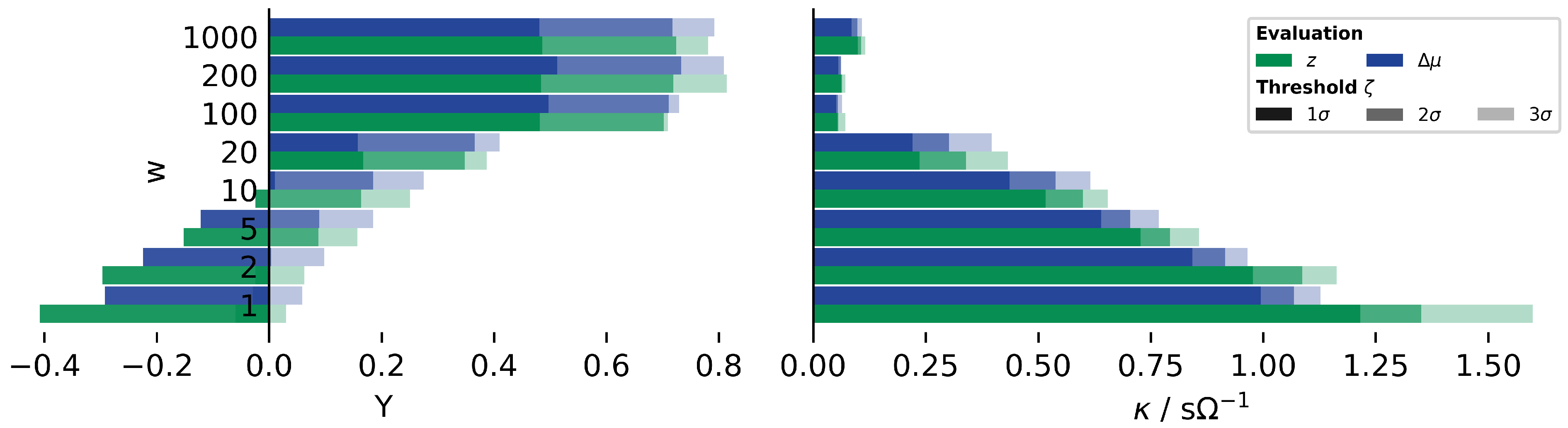
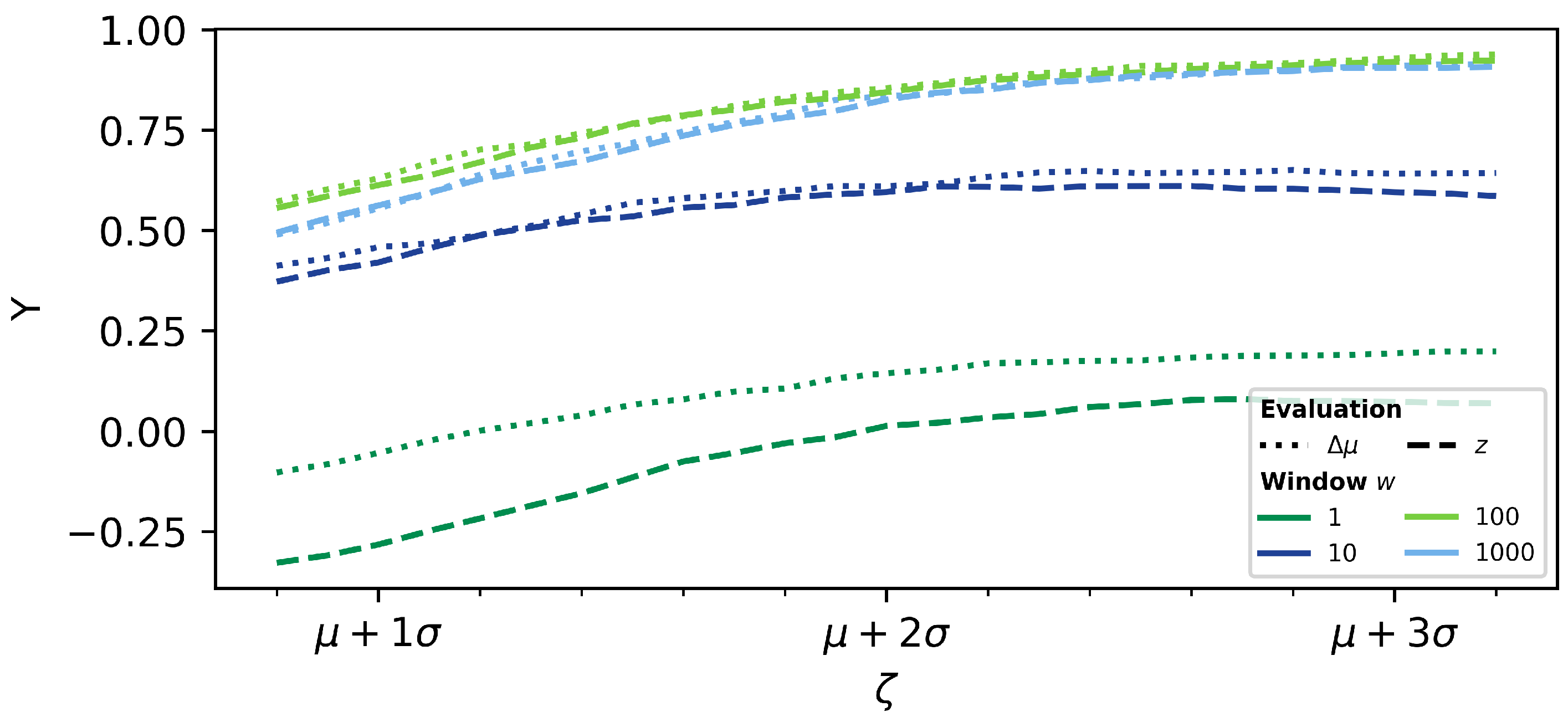
4.3. Fault Detection
4.4. Further Investigations
4.4.1. Threshold Level
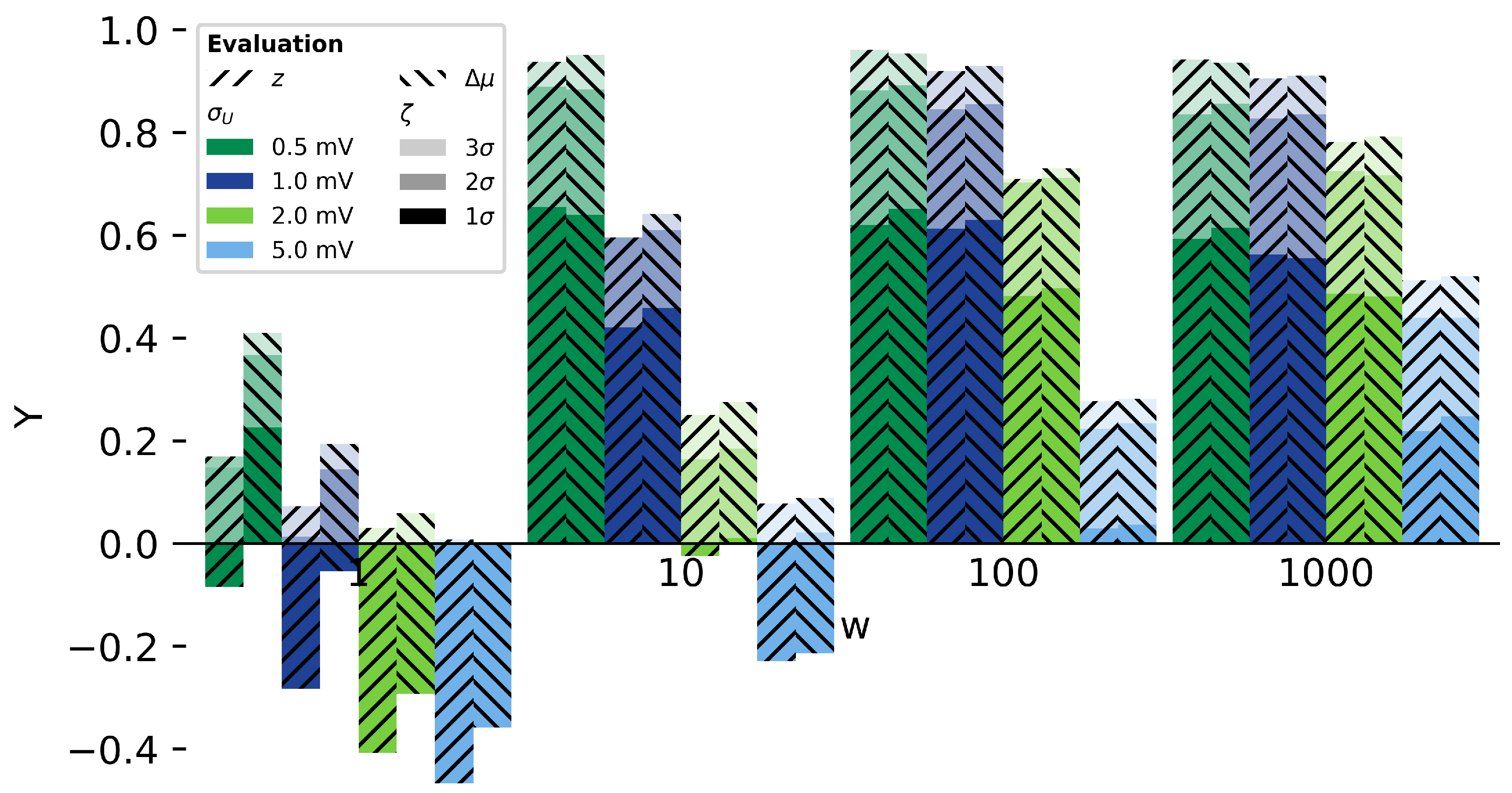
4.4.2. Noise Level
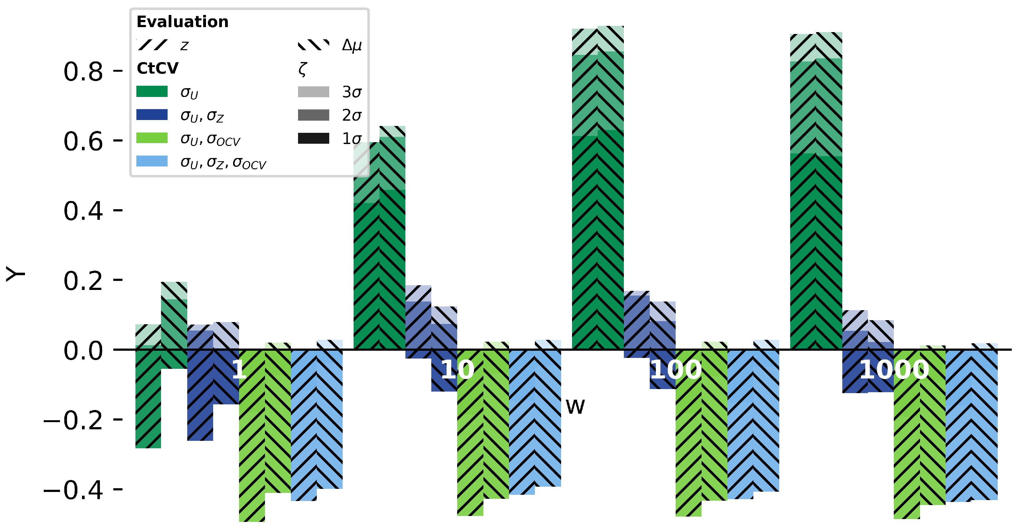
4.4.3. CtCV
5. Conclusions
Author Contributions
Funding
Institutional Review Board Statement
Informed Consent Statement
Data Availability Statement
Acknowledgments
Conflicts of Interest
Abbreviations
| BMS | Battery management system |
| CC | Constant current |
| CtCV | Cell-to-cell variation |
| CV | Coefficient of variation |
| ECM | Equivalent circuit model |
| ESC | External short circuit |
| EV | Electric vehicle |
| FNR | False negative rate (specificity) |
| FPR | False positive rate |
| GTR | Global Technical Regulation |
| GTR-EVS | Global Technical Regulation on Electrical Vehicle Safety |
| GUM | Guide to the expression of uncertainty in measurement |
| IC | Integrated circuit |
| ISC | Internal short circuit |
| LIB | Lithium-ion battery |
| LUT | Look-up-table |
| MA | Moving average |
| NPV | Negative predictive value |
| NRMSE | Normalized root mean squared error |
| OCV | Open circuit voltage |
| P2D | Pseudo two-dimensional |
| P-OCV | Pseudo open circuit voltage |
| PPV | Positive predictive value |
| RMS | Root mean square |
| RMSE | Root mean squared error |
| ROC | Receiver operating characteristic |
| SOC | State of Charge |
| SVM | Support vector machine |
| TNR | True negative rate |
| TPR | True positive rate (sensitivity) |
| TR | Thermal runaway |
| WLTP | Worldwide Harmonized Light-Duty Vehicles Test Procedure |
| Y | Youden-Index |
Appendix A
Appendix A.1. Evaluation of Computational Effort
| Listing 1. Implementation of the moving average algorithms using functions from pandas, NumPy and Numba. |
| import NumPy as np |
| from Numba import njit, prange, float64, int16 |
| def rollingMeanPandas(data, w=10): |
| return data.rolling(w).mean() |
| def rollingMeanNumPy(data, w=10): |
| result=np.empty_like(data) |
| for row in range(data.shape[0]): |
| window=np.zeros((w, data.shape[1])) |
| window[:]=np.nan # Initialise with np.nan |
| # Relevant for the first w rows |
| tmp=data[max(0,row−w+1):row+1, :] # Selection of data with window w |
| window[−len(tmp):, :]=tmp |
| result[row]= np.mean(window,axis=0) # Calculate mean over each column selection |
| return result |
| @njit(float64[:,:](float64[:,:],int16), parallel = True) # See above rollingMeanNumPy |
| def rollingMeanNumba(data, w=10): |
| result=np.empty_like(data) |
| for row in prange(data.shape[0]): |
| window=np.zeros((w, data.shape[1])) |
| window[:]=np.nan |
| tmp=data[max(0,row−w+1):row+1, :] |
| window[−len(tmp):, :]=tmp |
| avg=np.empty(window.shape[1], dtype=float64) |
| # np.mean(axis=0) is not implemented by Numba−>custom calculation |
| for col in range(window.shape[1]): |
| avg[col]=window[:,col].mean() |
| result[row]=avg |
| return result |
| Listing 2. Import of both functions and required packages. Random generation of test data with two different dimensions. |
| from SampleFunctions import ∗ |
| import pandas as pd |
| import NumPy as np |
| sampleData=np.random.rand(100000,12) |
| # SampleData=np.random.rand(100000,100) |
| sampleDF=pd.DataFrame(sampleData) |
| Listing 3. Evaluation of the computational time for each implemented function with respect to the required data structure. |
| timeit rollingMeanPandas(sampleDF, 10) |
| timeit rollingMeanNumba(sampleData, 10) |
| timeit rollingMeanNumPy(sampleData, 10) |
| Listing 4. Validation of correct implementation by pair-to-pair comparison of the calculated results based on the same random test data. |
| # Comparison of the evaluated arrays |
| print(np.allclose(rollingMeanNumba(sampleData, 10), |
| rollingMeanPandas(sampleDF, 10), equal_nan=True)) |
| print(np.allclose(rollingMeanNumPy(sampleData, 10), |
| rollingMeanPandas(sampleDF, 10), equal_nan=True)) |
| print(np.allclose(rollingMeanNumba(sampleData, 10), |
| rollingMeanNumPy(sampleData, 10), equal_nan=True)) |
| Specification | A | B |
|---|---|---|
| Processor | Intel Core i5-8265U | Intel Xeon W-2275 |
| Total cores | 4 | 14 |
| RAM | 8 GB | 256 GB |
| Year | 2020 | 2022 |
| A | B | |||
|---|---|---|---|---|
| Implementation | ||||
| Pandas | 114 ms | 63.7 ms | 41.3 ms | 573 ms |
| NumPy | 2.34 s | 1.93 s | 1.34 s | 1.56 s |
| Numba | 23.1 ms | 18.3 ms | 15.2 ms | 24.1 ms |
Appendix A.2. Consistency of Separate Simulation Studies
| FPR/% | TNR/% | FPR/% | TNR/% | ||||||||
|---|---|---|---|---|---|---|---|---|---|---|---|
| No | I | II | I | II | I | II | No | I | II | I | II |
| 1 | 3.108 | 3.110 | 0.167 | 0.167 | 99.833 | 99.833 | 1 | 0.600 | 0.832 | 99.400 | 99.168 |
| 10 | 1.369 | 1.364 | 1.000 | 0.833 | 99.000 | 99.167 | 10 | 2.183 | 3.854 | 97.817 | 96.146 |
| 100 | 0.408 | 0.408 | 1.083 | 1.500 | 98.917 | 98.500 | 100 | 3.523 | 2.474 | 96.477 | 97.526 |
| 1000 | 0.111 | 0.111 | 1.083 | 0.917 | 98.917 | 99.083 | 1000 | 1.394 | 2.053 | 98.606 | 97.947 |
References
- Yu, A.; Sumangil, M. Top Electric Vehicle Markets Dominate Lithium-ion Battery Capacity Growth; Technical Report; S&P Global Market Intelligence: New York, NY, USA, 2021. [Google Scholar]
- Feng, X.; Zheng, S.; Ren, D.; He, X.; Wang, L.; Cui, H.; Liu, X.; Jin, C.; Zhang, F.; Xu, C.; et al. Investigating the thermal runaway mechanisms of lithium-ion batteries based on thermal analysis database. Appl. Energy 2019, 246, 53–64. [Google Scholar] [CrossRef]
- Wang, Q.; Ping, P.; Zhao, X.; Chu, G.; Sun, J.; Chen, C. Thermal runaway caused fire and explosion of lithium ion battery. J. Power Sources 2012, 208, 210–224. [Google Scholar] [CrossRef]
- National Transportation Safety Board. Auxiliary Power Unit Battery Fire Japan Airlines Boeing 787-8, JA829J, Boston, MA 7 January 2013: Incident Report; Technical Report NTSB/AIR-14/01; National Transportation Safety Board: Washington, DC, USA, 2014.
- Koh, D.J. Samsung Announces Cause of Galaxy Note7 Incidents in Press Conference, Seoul, Republic of Korea, 23 January 2017. Available online: https://news.samsung.com/us/Samsung-Electronics-Announces-Cause-of-Galaxy-Note7-Incidents-in-Press-Conference (accessed on 11 October 2021).
- Meza, E. Several German Cities Halt Use of E-Buses Following Series of Unresolved Cases of Fire. Clean Energy Wire. Available online: https://www.cleanenergywire.org/news/german-cities-demand-subsidised-e-buses-outstrips-expectations (accessed on 11 October 2021).
- Naughton, K.; Yang, Y. GM Recalls All Bolt EVs on Fire Risk; Sees $1 Billion Cost. Available online: https://www.bloomberg.com/news/articles/2021-08-20/gm-to-spend-1-billion-to-recall-all-bolt-evs-due-to-fire-risk (accessed on 21 August 2021).
- Feng, X.; Fang, M.; He, X.; Ouyang, M.; Lu, L.; Wang, H.; Zhang, M. Thermal runaway features of large format prismatic lithium ion battery using extended volume accelerating rate calorimetry. J. Power Sources 2014, 255, 294–301. [Google Scholar] [CrossRef]
- Feng, X.; Ouyang, M.; Liu, X.; Lu, L.; Xia, Y.; He, X. Thermal runaway mechanism of lithium ion battery for electric vehicles: A review. Energy Storage Mater. 2018, 10, 246–267. [Google Scholar] [CrossRef]
- Li, H.; Duan, Q.; Zhao, C.; Huang, Z.; Wang, Q. Experimental investigation on the thermal runaway and its propagation in the large format battery module with Li(Ni1/3Co1/3Mn1/3)O2 as cathode. J. Hazard. Mater. 2019, 375, 241–254. [Google Scholar] [CrossRef] [PubMed]
- Zheng, S.; Wang, L.; Feng, X.; He, X. Probing the heat sources during thermal runaway process by thermal analysis of different battery chemistries. J. Power Sources 2018, 378, 527–536. [Google Scholar] [CrossRef]
- Ouyang, D.; Liu, J.; Chen, M.; Weng, J.; Wang, J. Thermal Failure Propagation in Lithium-Ion Battery Modules with Various Shapes. Appl. Sci. 2018, 8, 1263. [Google Scholar] [CrossRef]
- Ruiz, V.; Pfrang, A. JRC Exploratory Research: Safer Li-ion Batteries by Preventing Thermal Propagation; Technical Report; European Commission: Petten, The Netherlands, 2018. [Google Scholar]
- Klink, J.; Hebenbrock, A.; Grabow, J.; Orazov, N.; Nylén, U.; Benger, R.; Beck, H.P. Comparison of Model-Based and Sensor-Based Detection of Thermal Runaway in Li-Ion Battery Modules for Automotive Application. Batteries 2022, 8, 34. [Google Scholar] [CrossRef]
- Tidblad, A.A.; Edström, K.; Hernández, G.; de Meatza, I.; Landa-Medrano, I.; Jacas Biendicho, J.; Trilla, L.; Buysse, M.; Ierides, M.; Horno, B.P.; et al. Future Material Developments for Electric Vehicle Battery Cells Answering Growing Demands from an End-User Perspective. Energies 2021, 14, 4223. [Google Scholar] [CrossRef]
- Liu, B.; Jia, Y.; Li, J.; Yin, S.; Yuan, C.; Hu, Z.; Wang, L.; Li, Y.; Xu, J. Safety issues caused by internal short circuits in lithium-ion batteries. J. Mater. Chem. A 2018, 6, 21475–21484. [Google Scholar] [CrossRef]
- Doughty, D.H.; Pesaran, A.A. Vehicle Battery Safety Roadmap Guidance; Technical Report; National Renewable Energy Laboratory: Golden, CO, USA, 2012. [CrossRef]
- Liaw, B.Y.; Wang, F.; Wei, Y.; Brandt, K.; Schultheiß, J.; Schweizer-Berberich, M.; Dandl, S.; Wöhrle, T.; Lamp, P.; Jeevarajan, A.J.; et al. Managing Safety Risk by Manufacturers. In Li-Battery Safety; Garche, J., Brandt, K., Eds.; Electrochemical Power Sources; Elsevier: San Diego, CA, USA, 2019; pp. 267–378. [Google Scholar] [CrossRef]
- Lopez, C.F.; Jeevarajan, J.A.; Mukherjee, P.P. Experimental Analysis of Thermal Runaway and Propagation in Lithium-Ion Battery Modules. J. Electrochem. Soc. 2015, 162, A1905–A1915. [Google Scholar] [CrossRef]
- Zhong, G.; Li, H.; Wang, C.; Xu, K.; Wang, Q. Experimental Analysis of Thermal Runaway Propagation Risk within 18650 Lithium-Ion Battery Modules. J. Electrochem. Soc. 2018, 165, A1925–A1934. [Google Scholar] [CrossRef]
- Chen, F.; Huang, R.; Wang, C.; Yu, X.; Liu, H.; Wu, Q.; Qian, K.; Bhagat, R. Air and PCM cooling for battery thermal management considering battery cycle life. Appl. Therm. Eng. 2020, 173, 115154. [Google Scholar] [CrossRef]
- Kim, G.H.; Pesaran, A. Analysis of Heat Dissipation in Li-Ion Cells & Modules for Modeling of Thermal Runaway (Presentation). Available online: https://www.nrel.gov/docs/fy07osti/41531.pdf (accessed on 15 May 2007).
- Darcy, E. Driving Factors for Mitigating Cell Thermal Runaway Propagation and Arresting Flames in High Performing Li-Ion Battery Designs. Available online: https://ntrs.nasa.gov/api/citations/20150003488/downloads/20150003488.pdf (accessed on 1 May 2015).
- UN Global Technical Regulation. Global Technical Regulation No. 20: Global Technical Regulation on the Electrical Vehicle Safety (EVS); Technical Report; United Nations: Geneva, Switzerland, 2018. [Google Scholar]
- Schipper, F.; Erickson, E.M.; Erk, C.; Shin, J.Y.; Chesneau, F.F.; Aurbach, D. Review—Recent Advances and Remaining Challenges for Lithium Ion Battery Cathodes. J. Electrochem. Soc. 2017, 164, A6220–A6228. [Google Scholar] [CrossRef]
- Feng, X.; Ren, D.; He, X.; Ouyang, M. Mitigating Thermal Runaway of Lithium-Ion Batteries. Joule 2020, 4, 743–770. [Google Scholar] [CrossRef]
- Chombo, P.V.; Laoonual, Y. A review of safety strategies of a Li-ion battery. J. Power Sources 2020, 478, 228649. [Google Scholar] [CrossRef]
- Grabow, J.; Klink, J.; Benger, R.; Hauer, I.; Beck, H.P. Particle Contamination in Commercial Lithium-Ion Cells—Risk Assessment with Focus on Internal Short Circuits and Replication by Currently Discussed Trigger Methods. Batteries 2023, 9, 9. [Google Scholar] [CrossRef]
- Hu, X.; Zhang, K.; Liu, K.; Lin, X.; Dey, S.; Onori, S. Advanced Fault Diagnosis for Lithium-Ion Battery Systems: A Review of Fault Mechanisms, Fault Features, and Diagnosis Procedures. IEEE Ind. Electron. Mag. 2020, 14, 65–91. [Google Scholar] [CrossRef]
- Chen, Z.; Xu, K.; Wei, J.; Dong, G. Voltage fault detection for lithium-ion battery pack using local outlier factor. Measurement 2019, 146, 544–556. [Google Scholar] [CrossRef]
- Yao, L.; Xiao, Y.; Gong, X.; Hou, J.; Chen, X. A novel intelligent method for fault diagnosis of electric vehicle battery system based on wavelet neural network. J. Power Sources 2020, 453, 227870. [Google Scholar] [CrossRef]
- Chen, Z.; Xiong, R.; Tian, J.; Shang, X.; Lu, J. Model-based fault diagnosis approach on external short circuit of lithium-ion battery used in electric vehicles. Appl. Energy 2016, 184, 365–374. [Google Scholar] [CrossRef]
- Zhang, G.; Wei, X.; Tang, X.; Zhu, J.; Chen, S.; Dai, H. Internal short circuit mechanisms, experimental approaches and detection methods of lithium-ion batteries for electric vehicles: A review. Renew. Sustain. Energy Rev. 2021, 141, 110790. [Google Scholar] [CrossRef]
- Wu, C.; Zhu, C.; Ge, Y.; Zhao, Y. A Review on Fault Mechanism and Diagnosis Approach for Li-Ion Batteries. J. Nanomater. 2015, 2015, 631263. [Google Scholar] [CrossRef]
- Tran, M.K.; Fowler, M. A Review of Lithium-Ion Battery Fault Diagnostic Algorithms: Current Progress and Future Challenges. Algorithms 2020, 13, 62. [Google Scholar] [CrossRef]
- Bhaskar, K.; Kumar, A.; Bunce, J.; Pressman, J.; Burkell, N.; Rahn, C.D. Data-Driven Thermal Anomaly Detection in Large Battery Packs. Batteries 2023, 9, 70. [Google Scholar] [CrossRef]
- Liu, P.; Sun, Z.; Wang, Z.; Zhang, J. Entropy-Based Voltage Fault Diagnosis of Battery Systems for Electric Vehicles. Energies 2018, 11, 136. [Google Scholar] [CrossRef]
- Seo, M.; Goh, T.; Park, M.; Koo, G.; Kim, S. Detection of Internal Short Circuit in Lithium Ion Battery Using Model-Based Switching Model Method. Energies 2017, 10, 76. [Google Scholar] [CrossRef]
- Shang, Y.; Lu, G.; Kang, Y.; Zhou, Z.; Duan, B.; Zhang, C. A multi-fault diagnosis method based on modified Sample Entropy for lithium-ion battery strings. J. Power Sources 2020, 446, 227275. [Google Scholar] [CrossRef]
- Meng, J.; Boukhnifer, M.; Delpha, C.; Diallo, D. Incipient short-circuit fault diagnosis of lithium-ion batteries. J. Energy Storage 2020, 31, 101658. [Google Scholar] [CrossRef]
- Liu, Z.; He, H. Model-based Sensor Fault Diagnosis of a Lithium-ion Battery in Electric Vehicles. Energies 2015, 8, 6509–6527. [Google Scholar] [CrossRef]
- Schmid, M.; Kneidinger, H.G.; Endisch, C. Data-Driven Fault Diagnosis in Battery Systems Through Cross-Cell Monitoring. IEEE Sens. J. 2021, 21, 1829–1837. [Google Scholar] [CrossRef]
- Yao, L.; Wang, Z.; Ma, J. Fault detection of the connection of lithium-ion power batteries based on entropy for electric vehicles. J. Power Sources 2015, 293, 548–561. [Google Scholar] [CrossRef]
- Xue, Q.; Li, G.; Zhang, Y.; Shen, S.; Chen, Z.; Liu, Y. Fault diagnosis and abnormality detection of lithium-ion battery packs based on statistical distribution. J. Power Sources 2021, 482, 228964. [Google Scholar] [CrossRef]
- Zheng, Y.; Han, X.; Lu, L.; Li, J.; Ouyang, M. Lithium ion battery pack power fade fault identification based on Shannon entropy in electric vehicles. J. Power Sources 2013, 223, 136–146. [Google Scholar] [CrossRef]
- Yang, R.; Xiong, R.; He, H.; Chen, Z. A fractional-order model-based battery external short circuit fault diagnosis approach for all-climate electric vehicles application. J. Clean. Prod. 2018, 187, 950–959. [Google Scholar] [CrossRef]
- Chen, W.; Chen, W.T.; Saif, M.; Li, M.F.; Wu, H. Simultaneous Fault Isolation and Estimation of Lithium-Ion Batteries via Synthesized Design of Luenberger and Learning Observers. IEEE Trans. Control Syst. Technol. 2014, 22, 290–298. [Google Scholar] [CrossRef]
- Hong, J.; Wang, Z.; Liu, P. Big-Data-Based Thermal Runaway Prognosis of Battery Systems for Electric Vehicles. Energies 2017, 10, 919. [Google Scholar] [CrossRef]
- Seo, M.; Park, M.; Song, Y.; Kim, S.W. Online Detection of Soft Internal Short Circuit in Lithium-Ion Batteries at Various Standard Charging Ranges. IEEE Access 2020, 8, 70947–70959. [Google Scholar] [CrossRef]
- Xia, B.; Shang, Y.; Nguyen, T.; Mi, C. A correlation based fault detection method for short circuits in battery packs. J. Power Sources 2017, 337, 1–10. [Google Scholar] [CrossRef]
- Fill, A.; Koch, S.; Birke, K.P. Algorithm for the detection of a single cell contact loss within parallel-connected cells based on continuous resistance ratio estimation. J. Energy Storage 2020, 27, 101049. [Google Scholar] [CrossRef]
- Jiang, J.; Cong, X.; Li, S.; Zhang, C.; Zhang, W.; Jiang, Y. A Hybrid Signal-Based Fault Diagnosis Method for Lithium-Ion Batteries in Electric Vehicles. IEEE Access 2021, 9, 19175–19186. [Google Scholar] [CrossRef]
- Kang, Y.; Duan, B.; Zhou, Z.; Shang, Y.; Zhang, C. A multi-fault diagnostic method based on an interleaved voltage measurement topology for series connected battery packs. J. Power Sources 2019, 417, 132–144. [Google Scholar] [CrossRef]
- Zhang, H.; Pei, L.; Sun, J.; Song, K.; Lu, R.; Zhao, Y.; Zhu, C.; Wang, T. Online Diagnosis for the Capacity Fade Fault of a Parallel-Connected Lithium Ion Battery Group. Energies 2016, 9, 387. [Google Scholar] [CrossRef]
- Dey, S.; Mohon, S.; Pisu, P.; Ayalew, B. Sensor Fault Detection, Isolation, and Estimation in Lithium-Ion Batteries. IEEE Trans. Control Syst. Technol. 2016, 24, 2141–2149. [Google Scholar] [CrossRef]
- Dey, S.; Ayalew, B. A Diagnostic Scheme for Detection, Isolation and Estimation of Electrochemical Faults in Lithium-Ion Cells. In Proceedings of the ASME 8th Annual Dynamic Systems and Control Conference, Columbus, OH, USA, 29 October–3 November 2015; The American Society of Mechanical Engineers: New York, NY, USA, 2016. [Google Scholar] [CrossRef]
- Kang, Y.; Duan, B.; Zhou, Z.; Shang, Y.; Zhang, C. Online multi-fault detection and diagnosis for battery packs in electric vehicles. Appl. Energy 2020, 259, 114170. [Google Scholar] [CrossRef]
- Kim, G.H.; Smith, K.; Ireland, J.; Pesaran, A. Fail-safe design for large capacity lithium-ion battery systems. J. Power Sources 2012, 210, 243–253. [Google Scholar] [CrossRef]
- Kim, T.; Makwana, D.; Adhikaree, A.; Vagdoda, J.S.; Lee, Y. Cloud-Based Battery Condition Monitoring and Fault Diagnosis Platform for Large-Scale Lithium-Ion Battery Energy Storage Systems. Energies 2018, 11, 125. [Google Scholar] [CrossRef]
- Klink, J.; Grabow, J.; Orazov, N.; Benger, R.; Börger, A.; Ahlberg Tidblad, A.; Wenzl, H.; Beck, H.P. Thermal fault detection by changes in electrical behaviour in lithium-ion cells. J. Power Sources 2021, 490, 229572. [Google Scholar] [CrossRef]
- Kong, X.; Zheng, Y.; Ouyang, M.; Lu, L.; Li, J.; Zhang, Z. Fault diagnosis and quantitative analysis of micro-short circuits for lithium-ion batteries in battery packs. J. Power Sources 2018, 395, 358–368. [Google Scholar] [CrossRef]
- Li, X.; Wang, Z. A novel fault diagnosis method for lithium-Ion battery packs of electric vehicles. Measurement 2018, 116, 402–411. [Google Scholar] [CrossRef]
- Li, X.; Dai, K.; Wang, Z.; Han, W. Lithium-ion batteries fault diagnostic for electric vehicles using sample entropy analysis method. J. Energy Storage 2020, 27, 101121. [Google Scholar] [CrossRef]
- Sidhu, A.; Izadian, A.; Anwar, S. Adaptive Nonlinear Model-Based Fault Diagnosis of Li-Ion Batteries. IEEE Trans. Ind. Electron. 2015, 62, 1002–1011. [Google Scholar] [CrossRef]
- Singh, A.; Izadian, A.; Anwar, S. Fault diagnosis of Li-Ion batteries using multiple-model adaptive estimation. In Proceedings of the IECON 2013—39th Annual Conference of the IEEE Industrial Electronics Society, Vienna, Austria, 10–13 November 2013; Institute of Electrical and Electronics Engineers: New York, NY, USA, 2014; pp. 3524–3529. [Google Scholar] [CrossRef]
- Xia, B.; Nguyen, T.; Yang, J.; Mi, C. The improved interleaved voltage measurement method for series connected battery packs. J. Power Sources 2016, 334, 12–22. [Google Scholar] [CrossRef]
- Yan, W.; Zhang, B.; Wang, X.; Dou, W.; Wang, J. Lebesgue-Sampling-Based Diagnosis and Prognosis for Lithium-Ion Batteries. IEEE Trans. Ind. Electron. 2016, 63, 1804–1812. [Google Scholar] [CrossRef]
- Zhang, Z.; Kong, X.; Zheng, Y.; Zhou, L.; Lai, X. Real-time diagnosis of micro-short circuit for Li-ion batteries utilizing low-pass filters. Energy 2019, 166, 1013–1024. [Google Scholar] [CrossRef]
- Hong, J.; Wang, Z.; Yao, Y. Fault prognosis of battery system based on accurate voltage abnormity prognosis using long short-term memory neural networks. Appl. Energy 2019, 251, 113381. [Google Scholar] [CrossRef]
- Singh, A.; Izadian, A.; Anwar, S. Model based condition monitoring in lithium-ion batteries. J. Power Sources 2014, 268, 459–468. [Google Scholar] [CrossRef]
- Son, J.; Du, Y. Model-Based Stochastic Fault Detection and Diagnosis of Lithium-Ion Batteries. Processes 2019, 7, 38. [Google Scholar] [CrossRef]
- Tran, M.K.; Fowler, M. Sensor Fault Detection and Isolation for Degrading Lithium-Ion Batteries in Electric Vehicles Using Parameter Estimation with Recursive Least Squares. Batteries 2020, 6, 1. [Google Scholar] [CrossRef]
- Liu, Z.; Ahmed, Q.; Zhang, J.; Rizzoni, G.; He, H. Structural analysis based sensors fault detection and isolation of cylindrical lithium-ion batteries in automotive applications. Control Eng. Pract. 2016, 52, 46–58. [Google Scholar] [CrossRef]
- Moeini, A.; Wang, S. Fast and Precise Detection of Internal Short Circuit on Li-Ion Battery. In Proceedings of the 2018 IEEE Energy Conversion Congress and Exposition (ECCE), Portland, OR, USA, 23–27 September 2018; Institute of Electrical and Electronics Engineers: New York, NY, USA, 2018; pp. 2759–2766. [Google Scholar] [CrossRef]
- Ouyang, M.; Zhang, M.; Feng, X.; Lu, L.; Li, J.; He, X.; Zheng, Y. Internal short circuit detection for battery pack using equivalent parameter and consistency method. J. Power Sources 2015, 294, 272–283. [Google Scholar] [CrossRef]
- Xia, B.; Mi, C. A fault-tolerant voltage measurement method for series connected battery packs. J. Power Sources 2016, 308, 83–96. [Google Scholar] [CrossRef]
- Dey, S.; Biron, Z.A.; Tatipamula, S.; Das, N.; Mohon, S.; Ayalew, B.; Pisu, P. Model-based real-time thermal fault diagnosis of Lithium-ion batteries. Control Eng. Pract. 2016, 56, 37–48. [Google Scholar] [CrossRef]
- Wang, Y.; Tian, J.; Chen, Z.; Liu, X. Model based insulation fault diagnosis for lithium-ion battery pack in electric vehicles. Measurement 2019, 131, 443–451. [Google Scholar] [CrossRef]
- Liu, Z.; He, H. Sensor fault detection and isolation for a lithium-ion battery pack in electric vehicles using adaptive extended Kalman filter. Appl. Energy 2017, 185, 2033–2044. [Google Scholar] [CrossRef]
- Zhang, M.; Ouyang, M.; Lu, L.; He, X.; Feng, X.; Liu, L.; Xie, X. Battery Internal Short Circuit Detection. ECS Trans. 2017, 77, 217–223. [Google Scholar] [CrossRef]
- International Electrotechnical Commission. Uncertainty of Measurement: Part 3: Guide to the Expression of Uncertainty in Measurement (GUM:1995); ISO: Geneva, Switzerland, 2008. [Google Scholar]
- Mieke, S. Berechnung der Messunsicherheit nach GUM: Kurzfassung in 20 min. 2011. Available online: https://www.ptb.de/cms/fileadmin/internet/fachabteilungen/abteilung_8/8.4_mathematische_modellierung/277_PTB_SEMINAR/VORTRAEGE/11_Mieke_-_Berechnung_der_Messunsicherheit_nach_GUM__Kurzfassung_in_20.pdf (accessed on 7 May 2023).
- Zhao, S.; Duncan, S.R.; Howey, D.A. Observability Analysis and State Estimation of Lithium-Ion Batteries in the Presence of Sensor Biases. IEEE Trans. Control Syst. Technol. 2017, 25, 326–333. [Google Scholar] [CrossRef]
- Dirndorfer, T.; Botsch, M.; Knoll, A. Model-Based Analysis of Sensor-Noise in Predictive Passive Safety Algorithms. In Proceedings of the 22nd Enhanced Safety of Vehicles Conference, Washington, DC, USA, 13–16 June 2011; National Highway Traffic Safety Administration: Washington, DC, USA; p. 11-0251. [Google Scholar]
- Jerath, K.; Brennan, S.; Lagoa, C. Bridging the gap between sensor noise modeling and sensor characterization. Measurement 2018, 116, 350–366. [Google Scholar] [CrossRef]
- Marcicki, J.; Onori, S.; Rizzoni, G. Nonlinear Fault Detection and Isolation for a Lithium-Ion Battery Management System. In Proceedings of the ASME Dynamic Systems and Control Conference 2010, Cambridge, MA, USA, 12–15 September 2010; ASME: New York, NY, USA, 2010; pp. 607–614. [Google Scholar] [CrossRef]
- Zhang, C.; Allafi, W.; Dinh, Q.; Ascencio, P.; Marco, J. Online estimation of battery equivalent circuit model parameters and state of charge using decoupled least squares technique. Energy 2018, 142, 678–688. [Google Scholar] [CrossRef]
- Feng, X.; Weng, C.; Ouyang, M.; Sun, J. Online internal short circuit detection for a large format lithium ion battery. Appl. Energy 2016, 161, 168–180. [Google Scholar] [CrossRef]
- Alavi, S.M.M.; Fekriasl, S.; Niyakan, S.N.; Saif, M. Fault detection and isolation in batteries power electronics and chargers. J. Energy Storage 2019, 25, 100807. [Google Scholar] [CrossRef]
- Dey, S.; Perez, H.E.; Moura, S.J. Thermal fault diagnostics in Lithium-ion batteries based on a distributed parameter thermal model. In Proceedings of the 2017 American Control Conference (ACC), Seattle, WA, USA, 24–26 May 2017; Institute of Electrical and Electronics Engineers: New York, NY, USA, 2018; pp. 68–73. [Google Scholar]
- Dey, S.; Perez, H.E.; Moura, S.J. Model-Based Battery Thermal Fault Diagnostics: Algorithms, Analysis, and Experiments. IEEE Trans. Control Syst. Technol. 2019, 27, 576–587. [Google Scholar] [CrossRef]
- Pan, Y.; Feng, X.; Zhang, M.; Han, X.; Lu, L.; Ouyang, M. Internal short circuit detection for lithium-ion battery pack with parallel-series hybrid connections. J. Clean. Prod. 2020, 255, 120277. [Google Scholar] [CrossRef]
- Zhang, K.; Hu, X.; Liu, Y.; Lin, X.; Liu, W. Multi-fault Detection and Isolation for Lithium-Ion Battery Systems. IEEE Trans. Power Electron. 2022, 37, 971–989. [Google Scholar] [CrossRef]
- Wang, Z.; Hong, J.; Liu, P.; Zhang, L. Voltage fault diagnosis and prognosis of battery systems based on entropy and Z-score for electric vehicles. Appl. Energy 2017, 196, 289–302. [Google Scholar] [CrossRef]
- Analog Devices Inc. LTC6811-1/LTC6811-2: 12-Cell Battery Stack Monitor; Technical Report; Analog Devices Inc.: Wilmington, MA, USA, 2019. [Google Scholar]
- STMicroelectronics. Multicell Battery Monitoring and Balancing ICs. 2022. Available online: https://www.st.com/en/power-management/multicell-battery-monitoring-and-balancing-ics.html (accessed on 8 December 2022).
- Feng, F.; Hu, X.; Hu, L.; Hu, F.; Li, Y.; Zhang, L. Propagation mechanisms and diagnosis of parameter inconsistency within Li-Ion battery packs. Renew. Sustain. Energy Rev. 2019, 112, 102–113. [Google Scholar] [CrossRef]
- Könekamp, A.; Dudek, A.; Schilder, B. Cell Delta-Temperature Optimized Battery Module Configuration. U.S. Patent No 9,160,040, 13 October 2015. [Google Scholar]
- Joint Research Centre of the European Commission. Data Collection Framework: Definitions. 2023. Available online: https://www.wur.nl/en/research-results/statutory-research-tasks/centre-for-fisheries-research-1/data-collection-framework.htm (accessed on 5 June 2023).
- Dubarry, M.; Truchot, C.; Cugnet, M.; Liaw, B.Y.; Gering, K.; Sazhin, S.; Jamison, D.; Michelbacher, C. Evaluation of commercial lithium-ion cells based on composite positive electrode for plug-in hybrid electric vehicle applications. Part I: Initial characterizations. J. Power Sources 2011, 196, 10328–10335. [Google Scholar] [CrossRef]
- Kenney, B.; Darcovich, K.; MacNeil, D.D.; Davidson, I.J. Modelling the impact of variations in electrode manufacturing on lithium-ion battery modules. J. Power Sources 2012, 213, 391–401. [Google Scholar] [CrossRef]
- Rumpf, K.; Naumann, M.; Jossen, A. Experimental investigation of parametric cell-to-cell variation and correlation based on 1100 commercial lithium-ion cells. J. Energy Storage 2017, 14, 224–243. [Google Scholar] [CrossRef]
- Wildfeuer, L.; Lienkamp, M. Quantifiability of inherent cell-to-cell variations of commercial lithium-ion batteries. eTransportation 2021, 9, 100129. [Google Scholar] [CrossRef]
- Dubarry, M.; Vuillaume, N.; Liaw, B.Y. From single cell model to battery pack simulation for Li-ion batteries. J. Power Sources 2009, 186, 500–507. [Google Scholar] [CrossRef]
- Dubarry, M.; Vuillaume, N.; Liaw, B.Y. Origins and accommodation of cell variations in Li-ion battery pack modeling. Int. J. Energy Res. 2010, 34, 216–231. [Google Scholar] [CrossRef]
- Shin, D.; Poncino, M.; Macii, E.; Chang, N. A statistical model of cell-to-cell variation in Li-ion batteries for system-level design. In Proceedings of the International Symposium on Low Power Electronics and Design (ISLPED), Beijing, China, 4–6 September 2013; pp. 94–99. [Google Scholar] [CrossRef]
- Paul, S.; Diegelmann, C.; Kabza, H.; Tillmetz, W. Analysis of ageing inhomogeneities in lithium-ion battery systems. J. Power Sources 2013, 239, 642–650. [Google Scholar] [CrossRef]
- Baumhöfer, T.; Brühl, M.; Rothgang, S.; Sauer, D.U. Production caused variation in capacity aging trend and correlation to initial cell performance. J. Power Sources 2014, 247, 332–338. [Google Scholar] [CrossRef]
- Rothgang, S.; Baumhofer, T.; Sauer, D.U. Diversion of Aging of Battery Cells in Automotive Systems. In Proceedings of the 2014 IEEE Vehicle Power and Propulsion Conference (VPPC), Coimbra, Portugal, 27–30 October 2014; pp. 1–6. [Google Scholar]
- Schuster, S.F.; Brand, M.J.; Berg, P.; Gleissenberger, M.; Jossen, A. Lithium-ion cell-to-cell variation during battery electric vehicle operation. J. Power Sources 2015, 297, 242–251. [Google Scholar] [CrossRef]
- Devie, A.; Dubarry, M. Durability and Reliability of Electric Vehicle Batteries under Electric Utility Grid Operations. Part 1: Cell-to-Cell Variations and Preliminary Testing. Batteries 2016, 2, 28. [Google Scholar] [CrossRef]
- Campestrini, C.; Keil, P.; Schuster, S.F.; Jossen, A. Ageing of lithium-ion battery modules with dissipative balancing compared with single-cell ageing. J. Energy Storage 2016, 6, 142–152. [Google Scholar] [CrossRef]
- An, F.; Chen, L.; Huang, J.; Zhang, J.; Li, P. Rate dependence of cell-to-cell variations of lithium-ion cells. Sci. Rep. 2016, 6, 35051. [Google Scholar] [CrossRef]
- An, F.; Huang, J.; Wang, C.; Li, Z.; Zhang, J.; Wang, S.; Li, P. Cell sorting for parallel lithium-ion battery systems: Evaluation based on an electric circuit model. J. Energy Storage 2016, 6, 195–203. [Google Scholar] [CrossRef]
- Barreras, J.V.; Raj, T.; Howey, D.A.; Schaltz, E. Results of Screening over 200 Pristine Lithium-Ion Cells. In Proceedings of the 2017 IEEE Vehicle Power and Propulsion Conference (VPPC), Belfort, France, 14–17 December 2017; pp. 1–6. [Google Scholar] [CrossRef]
- Devie, A.; Baure, G.; Dubarry, M. Intrinsic Variability in the Degradation of a Batch of Commercial 18650 Lithium-Ion Cells. Energies 2018, 11, 1031. [Google Scholar] [CrossRef]
- Oeser, D.; Ziegler, A.; Ackva, A. Single cell analysis of lithium-ion e-bike batteries aged under various conditions. J. Power Sources 2018, 397, 25–31. [Google Scholar] [CrossRef]
- Baumann, M.; Wildfeuer, L.; Rohr, S.; Lienkamp, M. Parameter variations within Li-Ion battery packs—Theoretical investigations and experimental quantification. J. Energy Storage 2018, 18, 295–307. [Google Scholar] [CrossRef]
- Zou, H.; Zhan, H.; Zheng, Z. A Multi-Factor Weight Analysis Method of Lithiumion Batteries Based on Module Topology. In Proceedings of the 2018 International Conference on Sensing, Diagnostics, Prognostics, and Control (SDPC), Xi’an, China, 15–17 August 2018; pp. 61–66. [Google Scholar] [CrossRef]
- Zilberman, I.; Sturm, J.; Jossen, A. Reversible self-discharge and calendar aging of 18650 nickel-rich, silicon-graphite lithium-ion cells. J. Power Sources 2019, 425, 217–226. [Google Scholar] [CrossRef]
- Zilberman, I.; Ludwig, S.; Jossen, A. Cell-to-cell variation of calendar aging and reversible self-discharge in 18650 nickel-rich, silicon-graphite lithium-ion cells. J. Energy Storage 2019, 26, 100900. [Google Scholar] [CrossRef]
- Zilberman, I.; Schmitt, J.; Ludwig, S.; Naumann, M.; Jossen, A. Simulation of voltage imbalance in large lithium-ion battery packs influenced by cell-to-cell variations and balancing systems. J. Energy Storage 2020, 32, 101828. [Google Scholar] [CrossRef]
- Schindler, M.; Sturm, J.; Ludwig, S.; Schmitt, J.; Jossen, A. Evolution of initial cell-to-cell variations during a three-year production cycle. eTransportation 2021, 8, 100102. [Google Scholar] [CrossRef]
- Oeser, D. From the Production of the Single Cell to the End of Life of The Battery Module: The Development of Parameter Variation of Lithium-Ion Cells. Ph.D. Thesis, Departament d’Enginyeria Elèctrica, UPC, Barcelona, Spain, 2022. [Google Scholar]
- Reiter, A.; Lehner, S.; Bohlen, O.; Sauer, D.U. Electrical cell-to-cell variations within large-scale battery systems—A novel characterization and modeling approach. J. Energy Storage 2023, 57, 106152. [Google Scholar] [CrossRef]
- Hein, T.; Oeser, D.; Ziegler, A.; Montesinos-Miracle, D.; Ackva, A. Aging Determination of Series-Connected Lithium-Ion Cells Independent of Module Design. Batteries 2023, 9, 172. [Google Scholar] [CrossRef]
- Beck, D.; Dechent, P.; Junker, M.; Sauer, D.U.; Dubarry, M. Inhomogeneities and Cell-to-Cell Variations in Lithium-Ion Batteries, a Review. Energies 2021, 14, 3276. [Google Scholar] [CrossRef]
- Buchmann, I. BU-803a: Cell Matching and Balancing; Technical Report; Battery University: Richmond, BC, Canada, 2021. [Google Scholar]
- Barsukov, Y. Battery Cell Balancing: What to Balance and How; Technical Report; Texas Instruments: Dallas, TX, USA, 2022. [Google Scholar]
- Chang, L.; Zhang, C.; Wang, T.; Yu, Z.; Cui, N.; Duan, B.; Wang, C. Correlations of cell-to-cell parameter variations on current and state-of-charge distributions within parallel-connected lithium-ion cells. J. Power Sources 2019, 437, 226869. [Google Scholar] [CrossRef]
- Dubarry, M.; Pastor-Fernández, C.; Baure, G.; Yu, T.F.; Widanage, W.D.; Marco, J. Battery energy storage system modeling: Investigation of intrinsic cell-to-cell variations. J. Energy Storage 2019, 23, 19–28. [Google Scholar] [CrossRef]
- Song, Z.; Yang, X.G.; Yang, N.; Delgado, F.P.; Hofmann, H.; Sun, J. A study of cell-to-cell variation of capacity in parallel-connected lithium-ion battery cells. eTransportation 2021, 7, 100091. [Google Scholar] [CrossRef]
- Dubey, P.; Pulugundla, G.; Srouji, A.K. Direct Comparison of Immersion and Cold-Plate Based Cooling for Automotive Li-Ion Battery Modules. Energies 2021, 14, 1259. [Google Scholar] [CrossRef]
- Thakur, A.K.; Prabakaran, R.; Elkadeem, M.R.; Sharshir, S.W.; Arıcı, M.; Wang, C.; Zhao, W.; Hwang, J.Y.; Saidur, R. A state of art review and future viewpoint on advance cooling techniques for Lithium–ion battery system of electric vehicles. J. Energy Storage 2020, 32, 101771. [Google Scholar] [CrossRef]
- Eddahech, A.; Briat, O.; Vinassa, J.M. Thermal characterization of a high-power lithium-ion battery: Potentiometric and calorimetric measurement of entropy changes. Energy 2013, 61, 432–439. [Google Scholar] [CrossRef]
- Iraola, U.; Aizpuru, I.; Gorrotxategi, L.; Segade, J.M.C.; Larrazabal, A.E.; Gil, I. Influence of Voltage Balancing on the Temperature Distribution of a Li-Ion Battery Module. IEEE Trans. Energy Convers. 2015, 30, 507–514. [Google Scholar] [CrossRef]
- Jilte, R.D.; Kumar, R. Numerical investigation on cooling performance of Li-ion battery thermal management system at high galvanostatic discharge. Eng. Sci. Technol. Int. J. 2018, 21, 957–969. [Google Scholar] [CrossRef]
- Ni, P.; Wang, X. Temperature field and temperature difference of a battery package for a hybrid car. Case Stud. Therm. Eng. 2020, 20, 100646. [Google Scholar] [CrossRef]
- Shahid, S.; Agelin-Chaab, M. Analysis of Cooling Effectiveness and Temperature Uniformity in a Battery Pack for Cylindrical Batteries. Energies 2017, 10, 1157. [Google Scholar] [CrossRef]
- Tang, Z.; Wang, S.; Liu, Z.; Cheng, J. Numerical analysis of temperature uniformity of a liquid cooling battery module composed of heat-conducting blocks with gradient contact surface angles. Appl. Therm. Eng. 2020, 178, 115509. [Google Scholar] [CrossRef]
- DelRossi, R. Cell Balancing Design Guidelines. In Technical Report AN231; Microchip Technology Inc.: Chandler, AZ, USA, 2002. [Google Scholar]
- Ewert Energy Systems, I. How Cell Balancing Works. 2022. Available online: https://www.orionbms.com/manuals/utility_o2/param_balancing_description.html (accessed on 8 December 2022).
- Danae. Battery Pack Cell Voltage Difference and Solution: Part 1. 2021. Available online: https://www.grepow.com/blog/battery-pack-cell-voltage-difference-and-solution-part-1-battery-monday.html (accessed on 5 May 2023).
- Wang, Y.; Liu, D.; Shen, Y.; Tang, Y.; Chen, Y.; Zhang, J. Adaptive Balancing Control of Cell Voltage in the Charging/Discharging Mode for Battery Energy Storage Systems. Front. Energy Res. 2022, 10, 794191. [Google Scholar] [CrossRef]
- Brühl, M. Aktive Balancing-Systeme für Lithium-Ionen Batterien und deren Auswirkung auf die Zellalterung. Ph.D. Thesis, Université du Luxembourg, Luxemburg, 30 June 2017. [Google Scholar]
- Zhao, Y.; Liu, P.; Wang, Z.; Zhang, L.; Hong, J. Fault and defect diagnosis of battery for electric vehicles based on big data analysis methods. Appl. Energy 2017, 207, 354–362. [Google Scholar] [CrossRef]
- Gao, W.; Li, X.; Ma, M.; Fu, Y.; Jiang, J.; Mi, C. Case Study of an Electric Vehicle Battery Thermal Runaway and Online Internal Short-Circuit Detection. IEEE Trans. Power Electron. 2021, 36, 2452–2455. [Google Scholar] [CrossRef]
- Mallick, S.; Gayen, D. Thermal behaviour and thermal runaway propagation in lithium-ion battery systems—A critical review. J. Energy Storage 2023, 62, 106894. [Google Scholar] [CrossRef]
- Wikipedia contributors. Evaluation of Binary Classifiers. 2022. Available online: https://en.wikipedia.org/wiki/Evaluation_of_binary_classifiers (accessed on 7 May 2023).
- Hedderich, J.; Sachs, L. Angewandte Statistik; Springer: Berlin/Heidelberg, Germany, 2016. [Google Scholar] [CrossRef]
- Gao, W.; Zheng, Y.; Ouyang, M.; Li, J.; Lai, X.; Hu, X. Micro-Short-Circuit Diagnosis for Series-Connected Lithium-Ion Battery Packs Using Mean-Difference Model. IEEE Trans. Ind. Electron. 2019, 66, 2132–2142. [Google Scholar] [CrossRef]
- MathWorks. Matlab/Simulink. 2019. Available online: https://se.mathworks.com/products/simulink.html (accessed on 6 July 2020).
- Zhang, H.; Chow, M.Y. Comprehensive dynamic battery modeling for PHEV applications. In Proceedings of the IEEE PES General Meeting, Lake Buena Vista, FL, USA, 25–29 July 2010; pp. 1–6. [Google Scholar] [CrossRef]
- Lei, Y.; Jia, F.; Lin, J.; Xing, S.; Ding, S.X. An Intelligent Fault Diagnosis Method Using Unsupervised Feature Learning Towards Mechanical Big Data. IEEE Trans. Ind. Electron. 2016, 63, 3137–3147. [Google Scholar] [CrossRef]
- Sangwan, V.; Sharma, A.; Kumar, R.; Rathore, A.K. Equivalent circuit model parameters estimation of Li-ion battery: C-rate, SOC and temperature effects. In Proceedings of the 2016 IEEE International Conference on Power Electronics, Drives and Energy Systems (PEDES), Trivandrum, India, 14–17 December 2016; pp. 1–6. [Google Scholar] [CrossRef]
- Kong, X.; Plett, G.L.; Scott Trimboli, M.; Zhang, Z.; Qiao, D.; Zhao, T.; Zheng, Y. Pseudo-two-dimensional model and impedance diagnosis of micro internal short circuit in lithium-ion cells. J. Energy Storage 2020, 27, 101085. [Google Scholar] [CrossRef]
- Chen, M.; Bai, F.; Lin, S.; Song, W.; Li, Y.; Feng, Z. Performance and safety protection of internal short circuit in lithium-ion battery based on a multilayer electro-thermal coupling model. Appl. Therm. Eng. 2019, 146, 775–784. [Google Scholar] [CrossRef]
- Barai, A.; Tangirala, R.; Uddin, K.; Chevalier, J.; Guo, Y.; McGordon, A.; Jennings, P. The effect of external compressive loads on the cycle lifetime of lithium-ion pouch cells. J. Energy Storage 2017, 13, 211–219. [Google Scholar] [CrossRef]
- Cannarella, J.; Arnold, C.B. Stress evolution and capacity fade in constrained lithium-ion pouch cells. J. Power Sources 2014, 245, 745–751. [Google Scholar] [CrossRef]
- The SciPy community. SciPy. 2023. Available online: https://scipy.org/ (accessed on 7 May 2023).
- VDA Verband der Automobilindustrie. Abgasemissionen: WLTP—Weltweit Harmonisierter Zyklus für Leichte Fahrzeuge; VDA Verband der Automobilindustrie: Eisenach, Germany, 2020. [Google Scholar]
- Barnett, B. Lithium-Ion Cell Internal Shorting: 1. Early Detection 2. Simulation; National Transportation Safety Board (NTSB): Washington, DC, USA, 2017.
- Meng, J.; Boukhnifer, M.; Diallo, D. On-line Model-based Short Circuit Diagnosis of Lithium-Ion Batteries for Electric Vehicle Application. In Proceedings of the IECON 2019—45th Annual Conference of the IEEE Industrial Electronics Society, Chengdu, China, 15–17 December 2019; Institute of Electrical and Electronics Engineers: New York, NY, USA, 2019; pp. 6022–6027. [Google Scholar] [CrossRef]
- Seo, M.; Goh, T.; Koo, G.; Park, M.; Kim, S.W. Detection of Internal Short Circuit in Li-ion Battery by Estimating its Resistance. In Proceedings of the 4th IIAE International Conference on Intelligent Systems and Image Processing 2016, Kyoto, Japan, 8–12 September 2016; The Institute of Industrial Applications Engineers: Fukuoka, Japan, 2016; pp. 212–217. [Google Scholar] [CrossRef]
- Harris, C.R.; Millman, K.J.; van der Walt, S.J.; Gommers, R.; Virtanen, P.; Cournapeau, D.; Wieser, E.; Taylor, J.; Berg, S.; Smith, N.J.; et al. Array programming with NumPy. Nature 2020, 585, 357–362. [Google Scholar] [CrossRef] [PubMed]
- Virtanen, P.; Gommers, R.; Oliphant, T.E.; Haberland, M.; Reddy, T.; Cournapeau, D.; Burovski, E.; Peterson, P.; Weckesser, W.; Bright, J.; et al. SciPy 1.0: Fundamental algorithms for scientific computing in Python. Nat. Methods 2020, 17, 261–272. [Google Scholar] [CrossRef] [PubMed]
- The Pandas Development Team. Pandas-Dev/Pandas: Pandas. 2023. Available online: https://zenodo.org/record/7344967 (accessed on 7 May 2023).
- Ma, M.; Wang, Y.; Duan, Q.; Wu, T.; Sun, J.; Wang, Q. Fault detection of the connection of lithium-ion power batteries in series for electric vehicles based on statistical analysis. Energy 2018, 164, 745–756. [Google Scholar] [CrossRef]
- Guthrie, W.F. NIST/SEMATECH e-Handbook of Statistical Methods (NIST Handbook 151); Technical Report; National Institute of Standards and Technology: Gaithersburg, MA, USA, 2020. [CrossRef]
- Hansen, A. The Three Extreme Value Distributions: An Introductory Review. Front. Phys. 2020, 8, 604053. [Google Scholar] [CrossRef]
- Brodd, R.J. Batteries for Sustainability; Springer: New York, NY, USA, 2013. [Google Scholar] [CrossRef]
- Lai, X.; Jin, C.; Yi, W.; Han, X.; Feng, X.; Zheng, Y.; Ouyang, M. Mechanism, modeling, detection, and prevention of the internal short circuit in lithium-ion batteries: Recent advances and perspectives. Energy Storage Mater. 2021, 35, 470–499. [Google Scholar] [CrossRef]


| Author et al. | Source | |||
|---|---|---|---|---|
| Alavi | 0.316 | [89] * | ||
| Dey | 50 | 0.08 | 0.5 | [55] |
| Dey | 100 | 3.16 | 0.447 | [56] * |
| Dey | 5 | 10 | 0.3 | [90] |
| Dey | 5 | 10 | 0.3 | [91] |
| Feng | 2 | 0.1 | [88] | |
| Feng | 1 | 0.01 | [88] *,1 | |
| Kang | 100 | [53] *,2 | ||
| Kang | 100 | [57] *,2 | ||
| Kim | 10 | [59] | ||
| Pan | 10 | [92] *,2 | ||
| Shang | 10 | [39] * | ||
| Son | 450 | [71] | ||
| Xia | 1 | [50] | ||
| Zhang | 2 | 10 | [87] * | |
| Zhang | 2 | 25 | 0.05 | [93] |
| Zhao | 6 | [83] |
| Description | Value | Comment | Source | |
|---|---|---|---|---|
| Accuracy from analysed SMC-EV 1 platform | <10 mV | [94] | ||
| Accuracy from investigated EV | ±5 mV with resolution 1 mV | Cell voltage | [45] | |
| ±1 °C | Cell temperature | [45] | ||
| ±0.1 A if 30 A else ±1% | Pack current | [45] | ||
| ±1% | (±444 mV) | Pack voltage | [45] | |
| BMS accuracy of EV | ±0.1% | (±37 mV) | General assumption, no source | [57] |
| Standard deviation of investigated module | 0.3806 mV | Data from previous study; not published | [14] | |
| Accuracy from BMS-IC 2 | ±2.8 mV | Cell voltage, max. Value | [95] | |
| ±2.5% | ( ±1110 mV) | Pack voltage | [95] | |
| ±5 °C | Temperature | [95] | ||
| Accuracy from BMS-IC 2 | ±1.4 mV | Cell voltage | [96] | |
| Author et al. | Year | N | Cell | State | /Ah | /% | /% | Source |
|---|---|---|---|---|---|---|---|---|
| Dubarry | 2009 | 100 | - | - | 0.30 | - | 1.86 | [104] |
| 2010 | 100 | - | - | 0.30 | 30.12 | 1.86 | [105] | |
| 2011 | 10 | - | - | 1.90 | 5.66 | 0.16 | [100] | |
| Shin | 2013 | 10,000 | - | Model | - | 4.40 | 0.00 | [106] |
| Paul | 2013 | 20,000 | - | - | 4.40 | - | 1.30 | [107] |
| Zheng | 2013 | 96 | - | - | 70.00 | 19.47 | - | [45] |
| Baumhofer | 2014 | 48 | Sanyo/Panasonic UR18650E | - | 1.85 | - | 0.50 | [108] |
| Rothgang | 2014 | 700 | HP prismatic Cell | New | - | 2.87 | 2.36 | [109] |
| Schuster | 2015 | 954 | IHR18650A | Aged, from EV 2 | 1.95 | 3.19 | 1.57 | [110] |
| 2015 | 954 | IHR18650A | Aged, from EV 1 | 1.95 | 2.56 | 2.25 | [110] | |
| 2015 | 484 | IHR18650A | New | 1.95 | 1.94 | 0.80 | [110] | |
| Devie | 2016 | 100 | NCR 18650B | New | 3.35 | 0.30 | 0.80 | [111] |
| Campestrini | 2016 | 250 | Panasonic NCR18650PD | New | 2.80 | 0.72 | 0.16 | [112] |
| An | 2016 | 198 | - | - | 5.30 | 2.85 | 1.34 | [113] |
| 2016 | 7739 | - | - | 5.30 | - | 1.45 | [114] | |
| Rumpf | 2017 | 600 | Sony US26650FTC1 | New, Batch 1 | 3.00 | 1.81 | 0.23 | [102] |
| 2017 | 1100 | Sony US26650FTC1 | - | 3.00 | - | - | [102] | |
| Barreras | 2017 | 208 | SLPB 120216216 | New | 53.00 | 5.63 | 0.35 | [115] |
| Rumpf | 2017 | 500 | Sony US26650FTC1 | New, Batch 2 | 3.00 | 0.73 | 0.33 | [102] |
| Devie | 2018 | 51 | LG ICR18650 C2 | New | 2.80 | 3.55 | 2.00 | [116] |
| 2018 | 15 | LG ICR18650 C2 | Aged, 1000 cycles | 2.80 | 5.00 | 2.80 | [116] | |
| Oeser | 2018 | 50 | ICR 18650 26F | Aged, 1464 cycles, 77。8% SOH | 2.60 | - | 1.10 | [117] |
| Baumann | 2018 | 185 | BatteryPack, GS Yuasa (LEV50) | Aged, from EV | 50.00 | 4.40 | 0.85 | [118] |
| 2018 | 164 | Panasonic NCR18650PF | Aged, 3 years | 2.90 | 0.92 | 0.35 | [118] | |
| Zou | 2018 | 248 | - | New | 3.00 | 0.95 | 0.37 | [119] |
| Zilberman | 2019 | 13 | LG Chem INR18650-MJ1 | New | 3.50 | 1.08 | 0.22 | [120] |
| 2019 | 48 | LG MJ1 | New | 3.35 | 0.68 | 0.20 | [121] | |
| 2019 | 24 | LG MJ1 | Aged, 10 months | 3.35 | 0.75 | 0.38 | [121] | |
| 2020 | 48 | LG Chem INR18650-MJ1 | New | 3.35 | 0.79 | 0.20 | [122] | |
| Wildfeuer | 2021 | 568 | Sony US18650VTC5A | New | 2.50 | 0.86 | 0.24 | [103] |
| Schindler | 2021 | 48 | LG MJ1 | New, Batch 1 | 3.35 | 0.65 | 0.20 | [123] |
| 2021 | 200 | LG MJ1 | New, Batch 3 | 3.35 | 3.40 | 0.40 | [123] | |
| 2021 | 160 | LG MJ1 | New, Batch 2 | 3.35 | 1.04 | 0.36 | [123] | |
| Oeser | 2022 | 137 | ICR18650-26J | Aged, 2 years | 2.60 | 2.00 | 0.26 | [124] |
| 2022 | 480 | ICR18650-26J | New | 2.60 | 1.69 | 0.26 | [124] | |
| Reiter | 2023 | 14 | - | - | 128.00 | 2.20 | 0.39 | [125] |
| Hein | 2023 | 200 | ICR 18650-26J | - | 2.60 | 1.59 | 0.23 | [126] |
| Description | OCV/mV | Comment | Source |
|---|---|---|---|
| Guideline | 100 | Trigger for balancing | [141] |
| Guideline | 10 | Recommendation for | [142] |
| Guideline | 50 | Acceptable static voltage | [143] |
| 100 | Acceptable dynamic voltage | ||
| Application | 20 | Optimized balancing | [144] |
| Application | 100 | Common hysteresis | [128] |
| Application | 20 | Measurement of EV | [145] |
| 7 | Experimental balancing |
| Symbol | Name | Definition | Used in |
|---|---|---|---|
| TPR | True positive rate 1 | [40] | |
| FNR | False negative rate 2 | [40,41,63,73,79] | |
| TNR | True negative rate | ||
| FPR | False positive rate | [41,51,55,63,73,79] | |
| PPV | Positive predictive value | ||
| NPV | Negative predictive value | ||
| Y | Youden-index | TPR + FNR − 1 |
| Parameter | Symbol | Value |
|---|---|---|
| Nominal capacity | 10 Ah | |
| Nominal voltage | 3.7 V | |
| Upper voltage limit | 4.2 V | |
| Lower voltage limit | 2.7 V | |
| Charge current | | | 5 A|20 A |
| Discharge current | || | 5 A|20 A|30 A |
| Weight | m | 0.210 kg |
| Range | ||||||
|---|---|---|---|---|---|---|
| Distribution | Distribution | |||||
| Case | /mV | d/mV | /% | Parameter | Symbol | |
| Default () | 1.0 | 0.0 | 0.0 | Cell index of fault | k | * |
| Modified Default | 0.5, 1, 2 and 10 | 0.0 | 0.0 | Time of fault | ** | |
| or | 1.0 | 10 | 1.0 | Fault duration | ||
| and | 1.0 | 10 | 0.1 | Fault resistance |
| 2-Side/% | 1-Side/% | |
|---|---|---|
| 1 | 68.27 | 84.13 |
| 2 | 95.45 | 97.72 |
| 3 | 99.73 | 99.87 |
| Evaluation | /% | |||
|---|---|---|---|---|
| 1 | 5.84 | 1.56 | 33 | 3 |
| 2 | 5.45 | 3.28 | 29 | 11 |
| 5 | 6.24 | 5.24 | 38 | 27 |
| 10 | 5.70 | 5.37 | 32 | 28 |
| 20 | 6.48 | 6.29 | 41 | 38 |
| 100 | 8.76 | 8.02 | 74 | 62 |
| 200 | 8.31 | 7.85 | 67 | 60 |
| 1000 | 11.17 | 10.80 | 120 | 113 |
 | FPR/% | ||||||||
| Evaluation | z | z | z | z | |||||
| 1 | 0.004340 | 3.110 | 0.000241 | 0.051 | 1.053 | 0.079 | 0.833 | 0.167 | |
| 10 | 0.001349 | 1.364 | 0.000082 | 0.076 | 0.937 | 0.763 | 0.583 | 0.833 | |
| 100 | 0.000392 | 0.408 | 0.000032 | 0.033 | 0.932 | 0.935 | 1.083 | 1.500 | |
| 1000 | 0.000106 | 0.111 | 0.000011 | 0.011 | 0.624 | 0.669 | 0.583 | 0.917 | |
 | TPR | FPR | FNR | Youden | ||||||
| Evaluation | z | z | z | z | ||||||
| 1 | 1 | 0.208 | 0.336 | 0.491 | 0.391 | 0.792 | 0.664 | −0.283 | −0.055 | |
| 2 | 0.136 | 0.268 | 0.123 | 0.123 | 0.864 | 0.732 | 0.013 | 0.144 | ||
| 3 | 0.079 | 0.227 | 0.006 | 0.033 | 0.921 | 0.773 | 0.073 | 0.194 | ||
| 10 | 1 | 0.774 | 0.820 | 0.354 | 0.362 | 0.226 | 0.180 | 0.420 | 0.458 | |
| 2 | 0.686 | 0.731 | 0.091 | 0.121 | 0.314 | 0.269 | 0.596 | 0.610 | ||
| 3 | 0.617 | 0.665 | 0.022 | 0.024 | 0.383 | 0.335 | 0.595 | 0.642 | ||
| 100 | 1 | 0.966 | 0.966 | 0.353 | 0.337 | 0.034 | 0.034 | 0.613 | 0.630 | |
| 2 | 0.962 | 0.963 | 0.118 | 0.108 | 0.038 | 0.037 | 0.845 | 0.855 | ||
| 3 | 0.955 | 0.958 | 0.035 | 0.029 | 0.045 | 0.042 | 0.920 | 0.929 | ||
| 1000 | 1 | 0.941 | 0.946 | 0.379 | 0.391 | 0.059 | 0.054 | 0.562 | 0.555 | |
| 2 | 0.931 | 0.935 | 0.104 | 0.100 | 0.069 | 0.065 | 0.826 | 0.835 | ||
| 3 | 0.919 | 0.924 | 0.014 | 0.014 | 0.081 | 0.076 | 0.905 | 0.910 | ||
Disclaimer/Publisher’s Note: The statements, opinions and data contained in all publications are solely those of the individual author(s) and contributor(s) and not of MDPI and/or the editor(s). MDPI and/or the editor(s) disclaim responsibility for any injury to people or property resulting from any ideas, methods, instructions or products referred to in the content. |
© 2023 by the authors. Licensee MDPI, Basel, Switzerland. This article is an open access article distributed under the terms and conditions of the Creative Commons Attribution (CC BY) license (https://creativecommons.org/licenses/by/4.0/).
Share and Cite
Klink, J.; Grabow, J.; Orazov, N.; Benger, R.; Hauer, I.; Beck, H.-P. Systematic Approach for the Test Data Generation and Validation of ISC/ESC Detection Methods. Batteries 2023, 9, 339. https://doi.org/10.3390/batteries9070339
Klink J, Grabow J, Orazov N, Benger R, Hauer I, Beck H-P. Systematic Approach for the Test Data Generation and Validation of ISC/ESC Detection Methods. Batteries. 2023; 9(7):339. https://doi.org/10.3390/batteries9070339
Chicago/Turabian StyleKlink, Jacob, Jens Grabow, Nury Orazov, Ralf Benger, Ines Hauer, and Hans-Peter Beck. 2023. "Systematic Approach for the Test Data Generation and Validation of ISC/ESC Detection Methods" Batteries 9, no. 7: 339. https://doi.org/10.3390/batteries9070339
APA StyleKlink, J., Grabow, J., Orazov, N., Benger, R., Hauer, I., & Beck, H.-P. (2023). Systematic Approach for the Test Data Generation and Validation of ISC/ESC Detection Methods. Batteries, 9(7), 339. https://doi.org/10.3390/batteries9070339