State of Charge Estimation of Lithium-Ion Batteries Using the Window Attention Sinks Transformer

Abstract

Lithium-ion batteries are the core energy storage devices for electric vehicles, and accurate state of charge (SOC) estimation is critical to ensuring their safe and reliable operation. Most existing SOC estimation methods are only suitable for constant-temperature scenarios and cannot adapt to the dynamic temperature variations in actual charging and discharging processes. To address the issue of insufficient estimation accuracy under complex conditions such as high and low temperatures, this study proposes a Window Attention Sinks Transformer (WASFormer) model. Based on the PatchTST framework, the model integrates Rotary Positional Encoding (RoPE) and Window Attention Sinks (WAS) mechanisms, and combines Huber Loss with Reversible Instance Normalization (RevIN) to establish a full-chain robustness enhancement scheme from feature preprocessing to loss optimization, which effectively suppresses the interference of noise and distribution shift on estimation stability. Comparative experiments, generalization tests, and ablation studies under various temperatures and working conditions show that the proposed model achieves higher estimation accuracy, stronger generalization ability, and robustness. It provides an effective and stable new approach for high-precision SOC estimation of lithium-ion batteries over a wide temperature range and under complex operating conditions.

1. Introduction

With environmental pollution and the consumption of fossil fuels, the development of green and sustainable energy has become a global priority [1]. Due to their high energy density, long cycle life, and environmental friendliness, lithium-ion batteries have seen unprecedented opportunities for development in both research and application, and are widely used in energy storage systems and electric vehicles (EVs) [2]. In electric vehicles, the Battery Management System (BMS) serves as a key component responsible for maintaining battery safety and operational reliability. By continuously supervising and regulating battery conditions, including the State of Charge (SOC), State of Energy (SOE), and State of Health (SOH) [3], the BMS contributes to improved battery utilization and prolonged service life. SOC not only serves as a prediction target but also reflects the electrochemical state of the battery. It quantifies the charge stored in the electrodes and correlates with open-circuit voltage (OCV) under equilibrium conditions, providing a physically interpretable measure of battery energy content. Furthermore, SOC dynamics are influenced by internal polarization effects and temperature-dependent lithium-ion transport, which affect the voltage response and charge–discharge efficiency. Voltage, current, and temperature measurements therefore capture the combined effects of SOC, polarization, and thermal dynamics, forming the basis for both physical interpretation and data-driven SOC estimation models.

However, in practical applications, SOC is easily affected by battery nonlinearity, making it impossible to measure directly [4,5,6]; it must therefore be estimated using measurable parameters such as voltage, current, and temperature. Furthermore, battery performance is significantly affected by temperature fluctuations and variations in charging and discharging times [7,8]. In winter in certain high-latitude regions, where temperatures can drop as low as −20 °C, batteries may exhibit reduced capacity, resulting in overestimated SOC values. Conversely, during summer in regions near the equator, where maximum temperatures can reach 40 °C, battery capacity may experience intermittent increases, resulting in underestimated SOC values. This poses significant challenges to the accurate estimation of SOC.

Direct SOC estimation is commonly performed using ampere-hour counting and energy integration approaches [9]. Nevertheless, the accuracy of these methods strongly depends on the precision of the initial SOC value and sensor measurements. Any deviation in these inputs may accumulate over time, resulting in progressively larger estimation errors. Another widely adopted technique is the open-circuit voltage (OCV) method [10], which determines SOC according to the relationship between SOC and battery terminal voltage under equilibrium conditions. However, the requirement for a prolonged rest period before voltage measurement limits its applicability in real-time battery monitoring and control systems [11].

To overcome the shortcomings of direct estimation methods, researchers have developed model-based approaches that describe battery behavior through mathematical or equivalent circuit models. For instance, Oluwole et al. [12] proposed a fractional-order extended Kalman filter (IFO-EKF) derived from the conventional integer-order extended Kalman filter (IO-EKF), enabling dynamic SOC estimation under different operating conditions. Despite its improved estimation capability, the relatively slow response speed restricts its practical implementation. In addition, the Volterra integral dynamic model employs adaptive mechanisms to address battery load-balancing problems. Through load analysis experiments, Sidorov et al. [13] demonstrated the effectiveness of the Volterra-based framework for battery modeling and state estimation.

Unlike model-based approaches, data-driven methods estimate SOC directly from measurable operating data without requiring detailed knowledge of battery electrochemical characteristics or the establishment of complicated equivalent-circuit models [14,15,16]. By learning the relationship between historical operating information and battery states, these methods have become an important research direction in SOC estimation. Existing data-driven approaches can generally be divided into machine learning and deep learning categories. Representative machine learning algorithms include Gaussian Process Regression (GPR) [17], Support Vector Machines (SVM) [18], and Random Forests (RF) [19]. However, conventional machine learning techniques often exhibit limited capability when dealing with highly nonlinear battery behaviors, large-scale datasets, and long-term temporal dependencies, which restricts their estimation performance in practical applications.

To address these limitations, deep learning methods have been increasingly adopted for battery state estimation. Among them, Long Short-Term Memory (LSTM) and Gated Recurrent Unit (GRU) networks are widely used as fundamental architectures, with numerous studies introducing hybrid structures to further enhance prediction accuracy. For example, Fan et al. [20] integrated LSTM with Adaptive Unscented Kalman Filtering (AUKF), while Jiao et al. [21] developed a momentum-gradient-based GRU-RNN framework. Hu et al. [22] combined Temporal Convolutional Networks (TCN) and LSTM to exploit both local and sequential information. Experimental results demonstrated that these hybrid strategies generally outperform individual network models. Nevertheless, recurrent neural networks mainly emphasize short-term temporal patterns and often struggle to effectively model long-range dependencies in battery degradation sequences. To overcome this issue, attention mechanisms have been introduced into SOC estimation tasks. Tian et al. [23] incorporated an attention mechanism into an LSTM framework to better capture the interaction between voltage and current sequences, demonstrating the effectiveness of attention-assisted architectures. Similarly, Zou et al. [24] proposed a CNN-Informer hybrid model that utilizes attention mechanisms to extract spatial-temporal features from battery data and employs a Laplace-distribution-based loss function to improve robustness against measurement noise and outliers while enabling uncertainty quantification. Furthermore, Bian et al. [25] adopted an encoder–decoder framework for SOC prediction within the temperature range of 0–20 °C and achieved an MAE below 2.6%; however, further improvements in estimation accuracy remain desirable.

Despite the extensive research that has been conducted on the State of Charge (SOC) of lithium-ion batteries, maintaining a satisfactory balance between temperature adaptability and estimation accuracy remains challenging for existing methods, which may limit their effectiveness in practical forecasting applications [26,27]. In order to address this issue, the present study proposes a Window Attention Sinks Transformer (WASFormer) model. The integration of Rotary Positional Encoding (RoPE) with the Window Attention Sinks (WAS) mechanism within the PatchTST [28] architecture results in the construction of a forecasting framework that combines both local feature perception and global degradation modeling capabilities. Finally, the model’s estimation accuracy under different temperatures and operating conditions was validated using fit metrics and accuracy performance indicators, and it was compared with other advanced timeseries forecasting models. The findings demonstrate that WASFormer consistently exhibits superior estimation accuracy and can adapt to different temperature ranges across various operating conditions, exhibiting strong generalization capabilities. Moreover, experimental studies undertaken on the model corroborated the indispensability of each essential element and their collaborative effects.

2. Materials and Methods

2.1. SOC Estimation Process

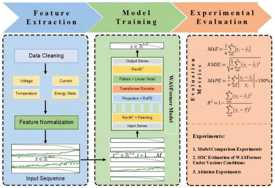
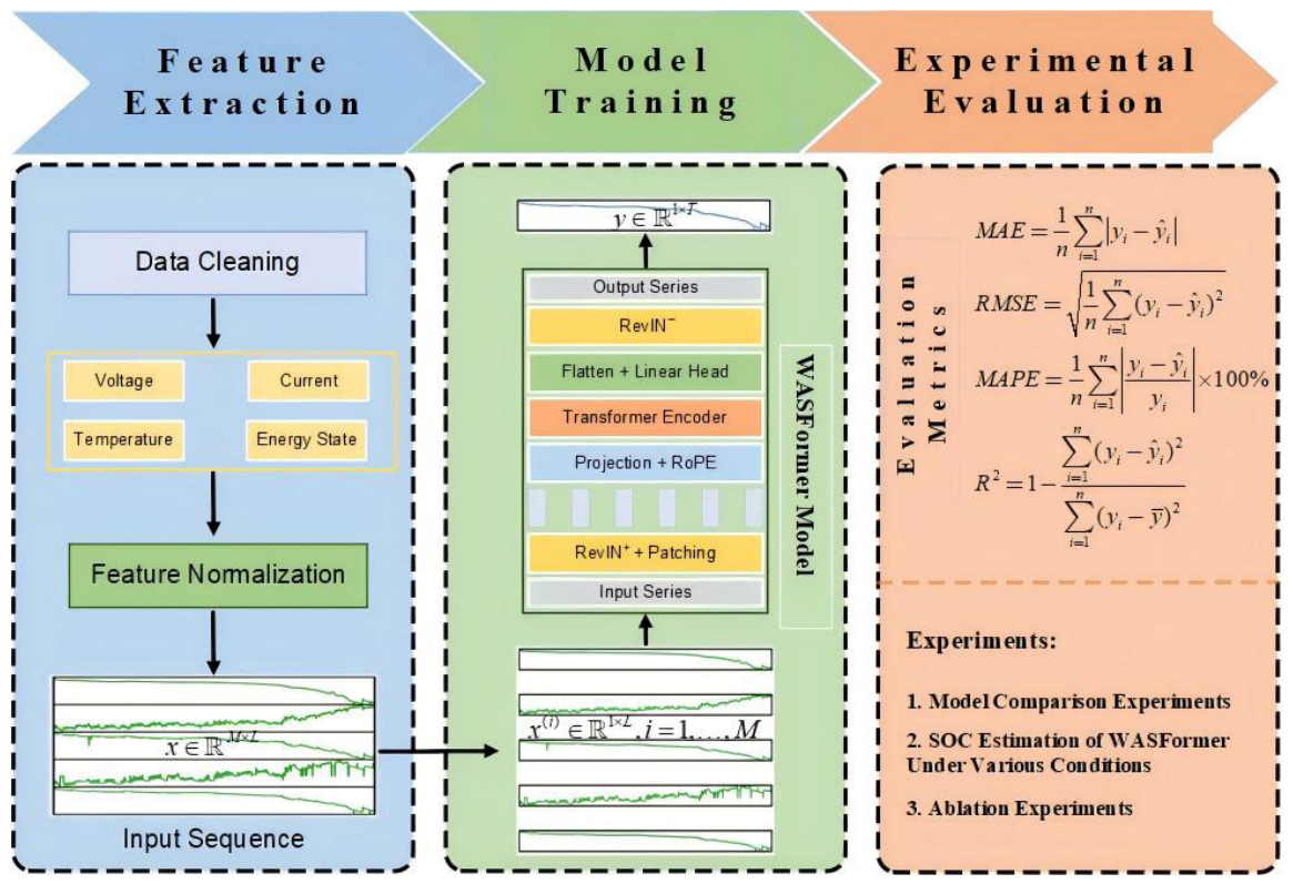
Figure 1 presents the flowchart of the proposed SOC estimation strategy. The voltage, current, and temperature inputs capture the combined effects of SOC, polarization, and thermal dynamics. This enables the WASFormer model to learn electrochemically meaningful temporal dependencies, rather than merely statistical correlations. The estimation process consists of three main steps: (1) collecting battery feature sequences during charging and discharging, followed by normalization; (2) inputting the processed feature sequences into the WASFormer model for training; (3) performing comparative experiments, evaluating model generalization under diverse operating conditions, and conducting ablation research.

2.2. WASFormer Model

To improve SOC estimation accuracy for lithium-ion batteries operating under diverse driving conditions and a broad temperature range, a novel Window Attention Sinks Transformer (WASFormer) framework is proposed in this study. Built upon the PatchTST architecture, the proposed model incorporates Rotary Positional Encoding (RoPE) and the Window Attention Sinks (WAS) mechanism to simultaneously characterize local dynamic variations and long-term degradation behaviors. First, a channel-independent strategy is adopted to decompose the multivariate input data into separate feature sequences, thereby alleviating the influence of inter-feature coupling. The extracted sequences are then enhanced by RoPE, which embeds relative positional relationships through rotational transformations and improves the representation of temporal dependencies. In addition, the WAS mechanism combines localized window-based attention with global information aggregation, enabling efficient feature extraction while suppressing the influence of noise. This design allows the model to effectively capture multi-scale temporal characteristics with reduced computational overhead. To further enhance robustness, Reversible Instance Normalization (RevIN) and Huber Loss are incorporated into the training framework, providing resilience against measurement noise and distribution shifts and ultimately improving prediction stability under complex operating conditions.

The specific prediction process can be described as follows: For a given lithium-ion battery feature sequence sample set with a look-back window $L:(x_1,\dots ,x_L)$, where each $x_t$ is a vector of dimension $M$ at each time step, used to predict the SOC value $y_{L+1}$ at the next future time point. The i-th extracted lithium-ion battery feature sequence can be represented as:

$$x_{1:L}^{(i)}=(x_1^{(i)},\dots ,x_L^{(i)}),i=1,\dots ,M$$

(1)

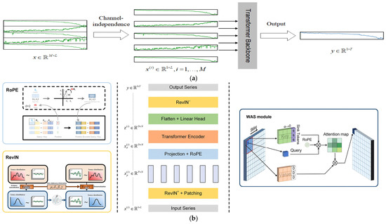
Subsequently, the input is segmented into $M$ unit sequences $x^{(i)}\in {ℝ}^{1\times L}$, which are independently fed into the Transformer Backbone through channel-independent mechanisms, producing output representations $z^{(i)}={ℝ}^{D\times N}$, where $D$ denotes the embedding dimension of the Transformer backbone and N denotes the number of generated patches. In this study, $D$ is set to 128. Under the adopted input configuration, the model uses the previous 12 samples (corresponding to 1.2 s of historical data with a sampling interval of 0.1 s) to predict the SOC at the next sampling instant. Therefore, the prediction horizon is $T=1$, and the output is represented as $y\in {ℝ}^{1\times T}$. The patching configuration used in the experiments results in $N=1$. The overall framework of the model is shown in Figure 2. Figure 2 presents an overview of the proposed WASFormer architecture. Since the figure is intended to provide a high-level illustration of the overall framework, the detailed structures and operational mechanisms of the main modules are further described in the subsequent figures and corresponding sections.

Before introducing the individual modules, the end-to-end learning process of WASFormer is briefly summarized to provide a high-level understanding of the model workflow. First, in the input preprocessing stage, the raw multivariate time-series signals are normalized using Reversible Instance Normalization (RevIN) to mitigate distribution shifts caused by varying operating conditions and temperature fluctuations, thereby providing distribution-stable inputs for subsequent learning. Second, in the sequence patching and embedding stage, the normalized sequences are partitioned into a series of local patches using a channel-independent strategy and projected into a high-dimensional embedding space, forming the basic input tokens for the Transformer backbone. Third, in the position-aware attention modeling stage, Rotary Positional Encoding (RoPE) is incorporated into the patch embeddings to encode relative positional information. The encoded representations are then processed by the Transformer backbone, where the proposed Window Attention Sinks (WAS) mechanism combines local window attention with Attention Sink tokens to effectively capture both fine-grained local temporal dependencies and robust global contextual information. Finally, in the output optimization stage, the predicted SOC values are restored to the original scale through the inverse RevIN transformation, while Huber Loss is employed as the optimization objective to improve training stability and robustness against outliers. The detailed principles and implementations of these components are presented in the following subsections.

2.2.1. Reversible Instance Normalization

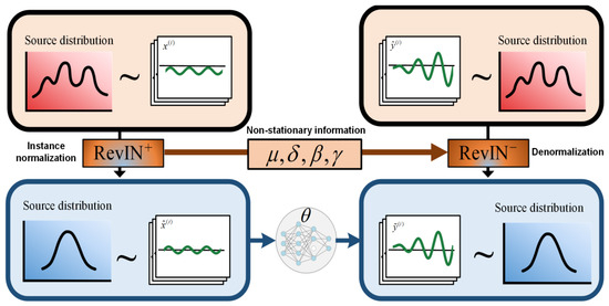
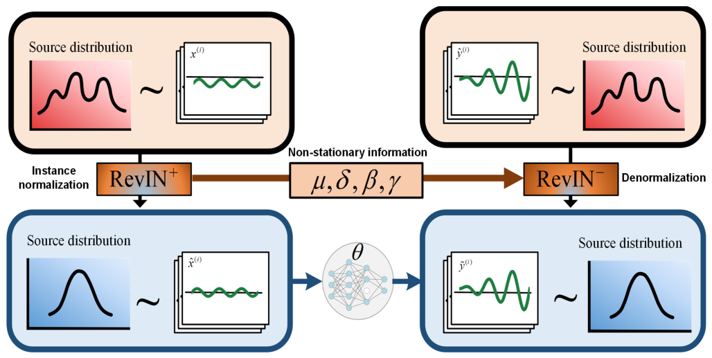
After obtaining each input feature sequence, this study employs the RevIN technique proposed by Kim et al. [29] to help mitigate the distribution shift between training and testing data, thereby improving prediction accuracy. Specifically, RevIN uses learnable affine transformations and a symmetric structure to remove and restore the statistical information of each feature sequence $x^{(i)}$. During forward propagation, it normalizes each $x^{(i)}$ before patching and then adds the mean and standard deviation back into the output prediction. The detailed workflow of RevIN is shown in Figure 3.

2.2.2. Patching

During patching, each input feature sequence $x^{(i)}$ is segmented into overlapping or non-overlapping patches. With patch length $P$ and stride $S$—the non-overlapping span between two consecutive patches—the overlap of patches is determined by $S$. After patching, a patch sequence $x_p^{(i)}\in {ℝ}^{P\times N}$ is produced, where the number of patches $N$ is given by:

$$N=[{\displaystyle \frac{(L-P)}{S}}]+1$$

(2)

The value $x_L^{(i)}\in ℝ$ ensures that the number of patches $N$ after partitioning satisfies the formula.

Through the patching operation, the number of input tokens decreases from $L$ to approximately $L/S$, which greatly reduces the model’s computational complexity, scaling down by the square of the stride $S$. This allows the model to process longer historical sequences to capture more meaningful temporal dependencies, thereby improving predictive performance.

2.2.3. Rotary Positional Encoding

Existing positional encoding methods can generally be categorized into absolute and relative approaches. Absolute positional encoding schemes, such as sinusoidal encoding and learnable embeddings, represent positional information by assigning unique vectors to different sequence locations. Although effective in preserving positional order, they are limited in their ability to explicitly characterize relative dependencies among sequence elements [30]. To address this limitation, relative positional encoding methods have been proposed. Representative approaches, such as ALiBi [31], incorporate distance-related information into the attention mechanism; however, they often rely on manually designed bias functions or additional attention modifications. As an alternative, Rotary Positional Encoding (RoPE) introduces positional information through rotational transformations in the feature space, enabling positional relationships to be naturally integrated into feature representations. This mechanism enhances the model’s capability to capture relative positional dependencies while maintaining computational efficiency in sequence modeling tasks. First, patches are projected into the embedding space by a learnable linear projection ${\mathrm{W}}_{\mathrm{p}}\in {ℝ}^{\mathrm{D}\times \mathrm{P}}$ to obtain the time-ordered sequence supervision for the learnable rotary positional encoding, yielding an output $x_d^{(i)}\in {ℝ}^{D\times N}$.

$$x_d^{(i)}={\mathrm{W}}_{\mathrm{p}}{x}_p^{(i)}{R}_m$$

(3)

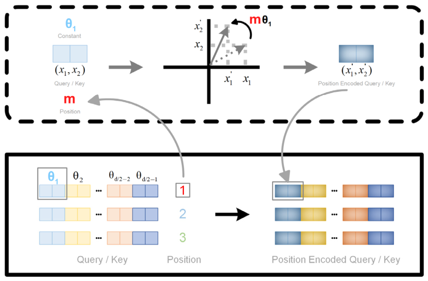
For each position $m$, the projected patches are encoded by the rotation matrix $R_m$ using RoPE, resulting in the position-aware representation:

$$R_m=\left(\begin{array}{ccccccc}\cos m{\theta }_0& -\sin m{\theta }_0& 0& 0& \dots & 0& 0\\ \sin m{\theta }_0& \cos m{\theta }_0& 0& 0& \dots & 0& 0\\ 0& 0& \cos m{\theta }_1& -\sin m{\theta }_1& \dots & 0& 0\\ 0& 0& \sin m{\theta }_1& \cos m{\theta }_1& \dots & 0& 0\\ ⋮& ⋮& ⋮& ⋮& \ddots & ⋮& ⋮\\ 0& 0& 0& 0& \dots & \cos m{\theta }_{d/2-1}& -\sin m{\theta }_{d/2-1}\\ 0& 0& 0& 0& \dots & \sin m{\theta }_{d/2-1}& \cos m{\theta }_{d/2-1}\end{array}\right),P=\left(\begin{array}{c}{p}_0\\ p_1\\ p_2\\ p_3\\ ⋮\\ \begin{array}{l}{p}_{d-2}\\ p_{d-1}\end{array}\end{array}\right)$$

(4)

Here, $P$ is the input vector matrix and $m$ is the position index; the rotation angle ${\theta }_i$ of each two-dimensional sub-vector is determined by the position index $m$ and the feature dimension $D$.

$${\theta }_i={\displaystyle \frac{1}{{\mathrm{10,000}}^{2(i-1)/d}}},\hspace{1em}i\in \{1,2,\dots ,d/2\}$$

(5)

This scheme links the rotation angle of every feature dimension directly to positional information.

In the subsequent encoder attention computation, the rotation matrices $R_m$ and $R_n$ transform the vectors $q$ and $k$ at positions $m$ and $n$ into $R_{m}q$ and $R_{n}k$, and the attention is computed on the transformed $Q$ and $K$ sequences. By evaluating the inner product after transformation, we obtain the following key identity.

$${(R_{m}q)}^{\mathrm{{\rm T}}}(R_{n}k)=q^{\mathrm{{\rm T}}}{R}_m^{\mathrm{{\rm T}}}{R}_{n}k=q^{\mathrm{{\rm T}}}{R}_{n-m}k$$

(6)

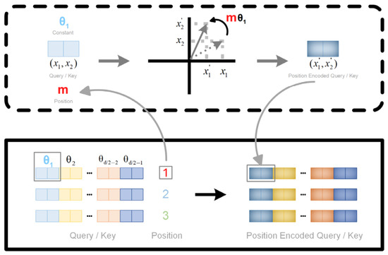
The transformed inner product implicitly encodes the positional difference $n-m$, enabling the attention mechanism to include relative positional information automatically without extra learning or manual biases, thus capturing positional correlations in sequences more effectively. The orthogonality of the rotation matrices ensures that the transformation preserves vector magnitudes, maintaining model stability, especially across deep network layers. The detailed implementation of RoPE is shown in Figure 4.

2.2.4. WAS Module

Local Window Attention [32] is a sparse attention mechanism that restricts the attention range to reduce computational complexity while strengthening the model’s ability to capture local features.

In traditional self-attention, each query vector $q_i$ interacts with all key vectors $k_i$ and value vectors $v_i$, leading to a complexity of $O(L^2)$ (where $L$ is the sequence length), which becomes prohibitive for long sequences. To mitigate this, Local Window Attention introduces an index matrix to confine each query to interact only with the keys and values within its local window. Specifically, each token’s receptive field is limited to its surrounding region; for an input sequence of length $L$ with a window size $W$, the attention at position $i$ only interacts with keys and values from positions $i-{\displaystyle \frac{W}{2}}$ to $i+{\displaystyle \frac{W}{2}}$.

$$Att{n}_i=soft\max \left({\displaystyle \frac{q_i\cdot k_{i-\frac{w}{2}:i+\frac{w}{2}}^{\mathrm{T}}}{\sqrt{d_k}}}\right)\cdot v_{i-{\displaystyle \frac{w}{2}}:i+{\displaystyle \frac{w}{2}}}$$

(7)

Here, $k_{i-{\displaystyle \frac{w}{2}}:i+{\displaystyle \frac{w}{2}}}$ and $v_{i-{\displaystyle \frac{w}{2}}:i+{\displaystyle \frac{w}{2}}}$ denote the sub-sequences of the key matrix $K$ and value matrix $V$ within the local window. This approach reduces the per-query complexity from $O(L)$ to $O(W)$, and lowers the overall complexity from $O(L^2)$ to $O(L\times W)$.

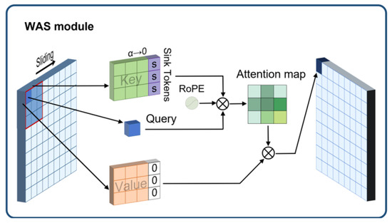
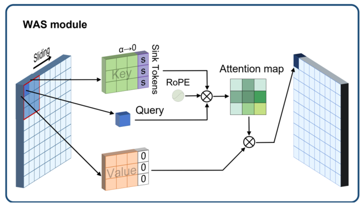
However, although Local Window Attention computes attention within local windows to markedly cut complexity, a fixed window size still cannot capture long-range dependencies and may miss salient information beyond the window [33]. It also risks overlooking boundary features. To address this, we incorporate the recently proposed Attention Sinks [34] technique from the LLM literature, which augments the attention key matrix with a special sink token $s$. This token absorbs unimportant signals and stabilizes the attention distribution, preventing certain tokens from being over-attended and thereby improving model robustness and predictive performance. Concretely, the window attention sinks (WAS) mechanism proposed in this study is illustrated in Figure 5, appends the sink token $s$ to the tail of the original key matrix $K$ and adds a zero vector to the tail of the value matrix $V$:

$$Att{n}_i=soft\max \left({\displaystyle \frac{q_i\cdot {[k_{i-\frac{w}{2}:i+\frac{w}{2}};s]}^{\mathrm{T}}}{\sqrt{d_k}}}\right)\cdot [v_{i-{\displaystyle \frac{w}{2}}:i+{\displaystyle \frac{w}{2}}};0]$$

(8)

This mechanism resembles the CLS token in BERT [35], but Attention Sinks focus more on absorbing noise; this design simultaneously reinforces the model’s robustness to global context information.

2.2.5. Huber Loss

As a special regression problem, lithium-ion battery SOC estimation involves data with complex dynamics and noise. During model training, choosing a suitable loss function is vital for enhancing model robustness, because traditional loss functions such as mean squared error (MSE) and mean absolute error (MAE) can yield prediction outcomes that lack resilience.

This study employs the Huber Loss function, which exhibits quadratic behavior for small residuals and linear behavior for large residuals. Its formulation is as follows:

$$L_{\delta }(g)=\left\{\begin{array}{ll}{\displaystyle \frac{1}{2}}{g}^2\hfill & if \left|g\right|\le \delta \hfill \\ \delta (|g|-{\displaystyle \frac{1}{2}}\delta )\hfill & otherwise\hfill \end{array}\right.,g=y_i-{\widehat{y}}_i$$

(9)

Here, $g$ denotes the error between the ground-truth value $y_i$ and the prediction ${\widehat{y}}_i$, $\delta$ is a margin parameter that balances Huber Loss between MSE and MAE. Specifically, when the error is small, Huber Loss resembles MSE Loss and retains smooth second-order differentiability, providing steady gradient information that enables faster convergence to the optimum. When the prediction error is large, Huber Loss transitions to the linear form of MAE Loss, reducing sensitivity to outliers and thus strengthening robustness while stabilizing training.

Selecting an appropriate $\delta$ is therefore important. In this work, $\delta$ is treated as a hyperparameter tuned via grid search, and ablation studies further verify the positive effect of Huber Loss.

3. Experiments and Analysis

3.1. Dataset and Correlation Analysist

The lithium-ion battery dataset used in this study originates from experiments conducted at the University of Wisconsin–Madison, using a brand-new 2.9 Ah NCA Panasonic 18650PF cell (Panasonic Corporation, Osaka, Japan), whose specifications are listed in

Table 1. Panasonic 18650PF Battery Specifications.

Battery Specifications	Value
Rated open-circuit voltage (V)	3.6
Rated capacity (Ah)	2.9
Charge Cut-off Voltage (V)	4.2
Cut-off voltage (V)	2.5

. The cell was charged at a 1C current until the voltage reached 4.2 V, followed by a constant-current–constant-voltage charge until the current tapered to 50 mA; this CC–CV protocol was repeated in every cycle. During testing, the battery underwent ten large charge–discharge loops. The dataset records cycling data under five driving schedules—HWFET, UDDS, LA92, US06, and NN—at ambient temperatures of −20 °C, −10 °C, 0 °C, 10 °C and 25 °C.

These operating conditions were selected to represent realistic battery usage scenarios in electric vehicles. Specifically, UDDS represents urban low-speed driving with frequent stop-and-go behavior, resulting in highly fluctuating current profiles. LA92 corresponds to a mixed urban/suburban driving condition with more aggressive acceleration and a wider current dynamic range. HWFET simulates highway cruising conditions characterized by relatively smooth current variations. US06 represents an aggressive high-speed driving cycle that includes rapid acceleration and deceleration events, leading to severe current transients. The NN cycle is a composite dynamic profile constructed from segments of US06 and LA92 with additional dynamic perturbations, incorporating characteristics of both urban and highway driving.

All voltage, current, temperature, and SOE signals were synchronously sampled at a fixed interval of 0.1 s, resulting in a total of 382,952 time steps. A sliding-window strategy with a window length of 12 and a stride of 1 was employed to construct the dataset. Each sample consists of 12 consecutive time steps of voltage, current, temperature, and SOE measurements, while the SOC value at the current time step serves as the prediction target. This procedure generated approximately 382,940 sample sequences.

The NN driving cycle data collected under five temperature conditions were used for training, whereas the HWFET, UDDS, LA92, and US06 datasets were used for testing. Each sample contains four input channels, namely voltage, current, temperature, and SOE. With a sampling interval of 0.1 s, the input window corresponds to 1.2 s of historical observations, which is sufficient to capture short-term battery dynamics under varying operating conditions while maintaining computational efficiency.

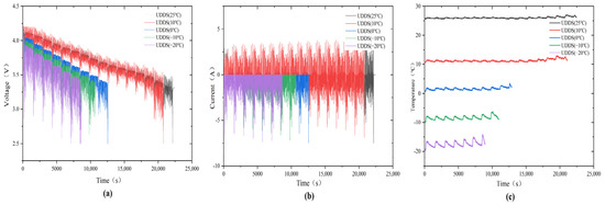
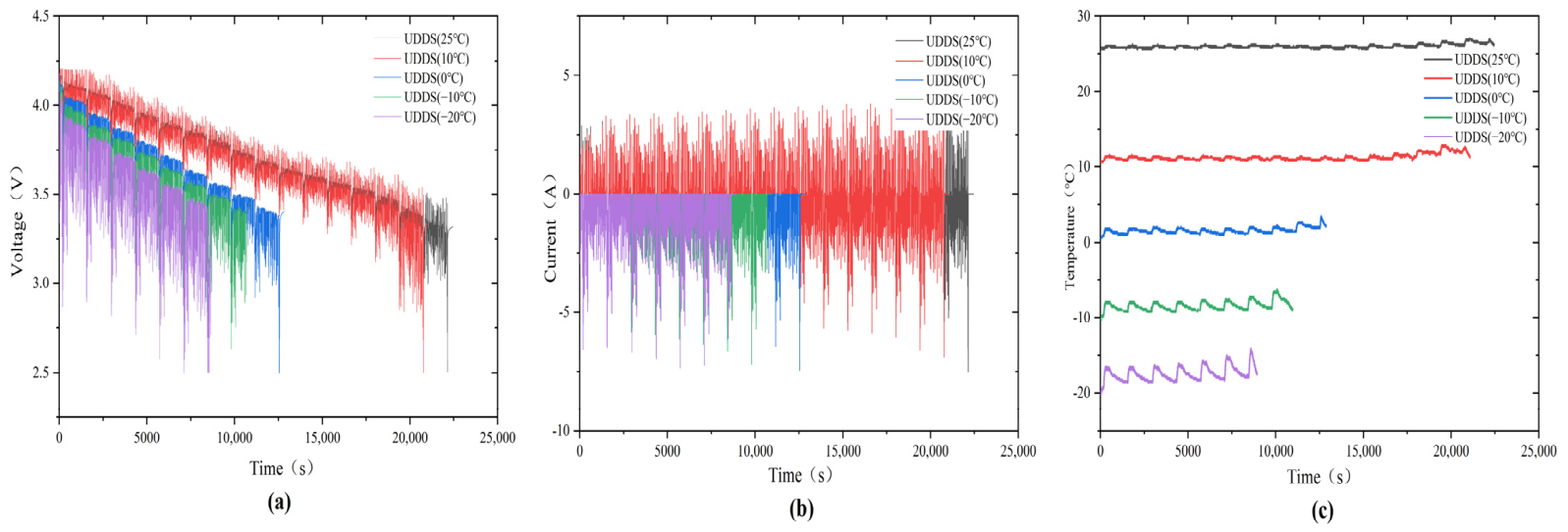
The SOC labels provided in the dataset were calculated using the ampere-hour integration (coulomb counting) method. The voltage, current, temperature, and state of energy (SOE) data from the lithium-ion battery are used as model inputs to accurately estimate the SOC. It should be noted that the State of Energy (SOE) used as an input feature is computed from the measured voltage, current, and temperature sequences according to standard BMS energy integration procedures. While SOC and SOE are related, SOE reflects cumulative energy dynamics over time rather than instantaneous charge, providing complementary temporal information. By treating SOE as an independent input channel, the model leverages additional energy-related features without introducing direct redundancy with SOC. To ensure consistency and training stability, the training data is normalized to the range of 0–1. Taking the UDDS as an example, its voltage, current, and temperature distributions are shown in Figure 6. All voltage, current, and temperature data are sampled every 0.1 s.

The formulas defining and SOE are as follows:

$$SO{E}_t=SO{E}_{t_0}-{\displaystyle \frac{{\displaystyle {\int }_{t_0}^t{U}_t\cdot I_{t}dt}}{E_n}}$$

(10)

where $t$ represents the current moment, $t_0$ represents the initial discharge time, $I_t$ is the load current at the current moment, $U_t$ is the terminal voltage of the battery, $E_n$ represents the rated total energy of the battery. SOE is more concerned with the energy that the battery can provide under the current operating conditions, providing a decision basis for energy optimization and power scheduling.

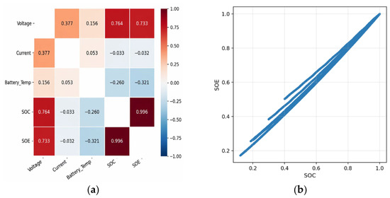
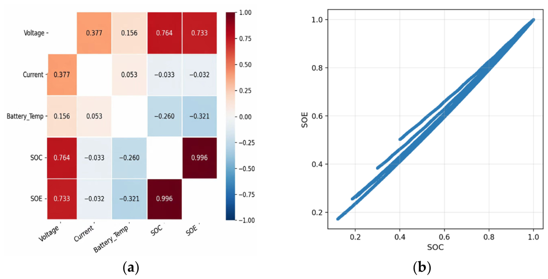
Figure 7 shows the results of the Spearman rank correlation analysis between the various input features. It can be seen that SOC and voltage as well as SOE and voltage exhibit strong positive correlations, while the correlations between current and temperature and the other features are relatively weak. This indicates that each feature describes the battery state from a different dimension. The relatively weak correlations of current and temperature with SOC can be attributed to the fact that these variables primarily act as external operating factors that influence battery dynamics rather than directly determining the SOC value itself. Their effects on SOC are often indirect and nonlinear, resulting in relatively low pairwise correlation coefficients.

Although SOC and SOE show a strong positive correlation overall, the scatter plot does not converge into a single straight line but instead exhibits a distinct multi-band distribution. This indicates that SOE takes on different values at the same SOC level, reflecting the impact of operational conditions such as temperature and internal resistance on the actual available energy. This high correlation stems from their shared monotonically decreasing trend rather than redundant information; SOE still provides irreplaceable complementary information for SOC estimation. Furthermore, the relatively weak correlations of current and temperature demonstrate that feature importance cannot be evaluated solely based on correlation coefficients, highlighting the necessity of deep learning models for extracting complex nonlinear relationships among battery variables.

3.2. Experimental Setup

This study evaluates the overall performance of the proposed WASFormer model through three aspects: model comparison experiments, generalization tests, and ablation study. To quantitatively assess prediction performance from different perspectives, four commonly adopted regression metrics are employed. In all experiments, the data values are presented as percentages. The formulas for these evaluation metrics are as follows:

$$MAE={\displaystyle \frac{1}{n}}{\displaystyle \sum _{i=1}^n\left|y_i-{\widehat{y}}_i\right|}$$

(11)

$$RMSE=\sqrt{{\displaystyle \frac{1}{n}}{\displaystyle \sum _{i=1}^n{(y_i-{\widehat{y}}_i)}^2}}$$

(12)

$$MAPE={\displaystyle \frac{1}{n}}{\displaystyle \sum _{i=1}^n\left|\frac{y_i-{\widehat{y}}_i}{y_i}\right|}\times 100\%$$

(13)

$$R^2=1-{\displaystyle \frac{{\displaystyle \sum _{i=1}^n{(y_i-{\widehat{y}}_i)}^2}}{{\displaystyle \sum _{i=1}^n{(y_i-\overline{y})}^2}}}$$

(14)

Here, $n$ is the number of cycles from the start of prediction to termination; $y_i$ denotes the true capacity value, ${\widehat{y}}_i$ the predicted capacity, and $\overline{y}$ the mean of the true values. Smaller MAE, RMSE, and MAPE indicate higher predictive accuracy, while an R² closer to 1 signifies better predictions.

To minimize loss, we adopt the AdamW optimizer and introduce the weight-decay coefficient as a hyperparameter to promote better convergence and generalization. To further accelerate convergence and boost training efficiency, we employ the OneCycleLR learning-rate scheduler, which divides the full training horizon into a warm-up phase and a decay phase. During warm-up, the learning rate increases linearly from the initial value $l_0$ to the maximum value $m$; the fraction of total steps spent in this phase is controlled by parameter $p$ (default 30%). During decay, the learning rate follows a cosine schedule down to the final value $f_{lr}$, computed as $l_0$ divided by factor $f$ (default 10,000). The learning rate scheduling formula can be expressed as:

$$lr(t)=\left\{\begin{array}{ll}{l}_0+{\displaystyle \frac{m-l_0}{p\cdot T}}\cdot t,\hfill & if t\le p\cdot T\hfill \\ f_{lr}+{\displaystyle \frac{1}{2}}\left(m-f_{lr}\right)\left(1+\cos \left({\displaystyle \frac{t-p\cdot T}{(1-p)\cdot T}}\cdot \pi \right)\right),\hfill & otherwise\hfill \end{array}\right.$$

(15)

Here, $T$ denotes the total number of training steps, obtained by multiplying the number of epochs with the steps per epoch (defaulting to the length of the training set); $t$ is the current step. It is worth noting that $l_0$ and $m$ represent the initial learning rate $lr$ and the upper limit of the learning rate $\max lr$ in the hyperparameters, respectively. The results in this paper are based on the average of 10 experiments conducted with different random seeds. This is a widely used and rigorous experimental method in the field of time series forecasting, which helps mitigate experimental randomness and variability.

During model training, the proper configuration of hyperparameters is crucial to model performance. Adaptive optimization algorithms can often identify the optimal combination of network hyperparameters, thereby making the network architecture more rational and efficient. These algorithms also prevent the model from getting stuck in local optima due to manual parameter tuning. In this study, we used the probability-based Tree-structured Parzen Estimator (TPE) [36] method to perform hyperparameter optimization on all models included in the experiments. The search spaces for each hyperparameter are shown in

Table 2. Hyperparameter information for TPE optimization.

-	Hyperparameters	Parameter Description	Search Space
Model Parameters	n_layers	Number of encoder layers	[2, 3, 4, 5, 6]
	n_heads	Number of Attention Points	[2, 4, 6, 8]
	fc_dropout	FC Layer Drop Rate	[0.05, 0.5]
	head_dropout	Discard rate for each head	[0.05, 0.5]
	d_model	Feature Embedding Dimension	[32, 64, 128]
	d_ff	FNN Layer Dimension	[64, 128, 256]
	weight decay	Weight decay coefficient	[1 ×10−5, 1 × 10−1]
Train Parameters	lr	Learning rate	[1× 10−5, 1× 10−2]
	max lr	Maximum learning rate	[1× 10−4, 1× 10−1]
	delta	Loss Threshold Parameter	[0.1, 2.0]

. In all experiments, Train Parameters were optimized, while the model proposed in this study additionally optimized the WASFormer model hyperparameters listed under Model Parameters. Furthermore, the number of trials was fixed at 500, the batch size was set to 32, and the number of epochs was set to 500. To accelerate the training process, an early stopping mechanism was implemented.

3.3. Experimental Analysis

3.3.1. Comparative Experiment

To investigate the performance of hybrid deep learning models for SOC estimation under varying temperature conditions, this study compares the proposed WASFormer model with several state-of-the-art time series forecasting models, including iTransformer [37], Informer [38], GRU [39], NLinear, and DLinear [40]. To further evaluate the practical relevance of the proposed method, a conventional SOC estimation approach based on the Extended Kalman Filter (EKF) is introduced as a benchmark. The EKF method is widely used in battery SOC estimation and represents a typical physics-based estimation framework.

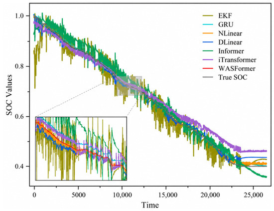
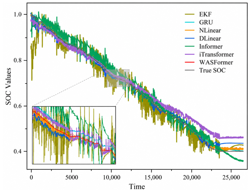
Specifically, all models are evaluated at five temperature conditions (−20 °C, −10 °C, 0 °C, 10 °C, and 25 °C) to assess their ability to estimate SOC under diverse environmental conditions.

Table 3. SOC estimation results of each model for five different temperature conditions under US06 operating condition.

Temperature	Metrics	WASFormer	iTransformer	Informer	GRU	NLiner	DLiner	EKF
−20 °C	MAE (%)	0.027	2.756	2.189	0.803	0.454	1.133	1.726
	RMSE (%)	0.032	3.504	2.535	0.913	0.606	1.607	2.981
	MAPE (%)	0.043	5.477	3.459	1.442	0.865	2.151	2.671
	R2 (%)	99.99971	96.55710	98.19816	99.76618	99.89715	99.27582	97.50828
−10 °C	MAE (%)	0.054	2.123	1.102	0.678	0.333	0.863	4.846
	RMSE (%)	0.059	2.556	1.391	0.787	0.401	1.035	6.143
	MAPE (%)	0.105	4.632	1.799	1.478	0.656	1.727	8.078
	R2 (%)	99.99925	98.60430	99.58668	99.86756	99.96560	99.77111	91.94048
0 °C	MAE (%)	0.086	2.067	2.791	0.478	0.490	1.218	3.082
	RMSE (%)	0.089	2.276	3.467	0.562	0.577	1.406	3.791
	MAPE (%)	0.196	4.466	7.783	1.054	1.031	2.698	7.132
	R2 (%)	99.99870	99.14259	98.01074	99.94771	99.94491	99.67274	97.62135
10 °C	MAE (%)	0.124	1.899	5.684	0.305	0.394	0.982	2.277
	RMSE (%)	0.127	2.086	6.496	0.437	0.482	1.180	2.781
	MAPE (%)	0.264	3.475	13.902	0.646	0.768	1.900	5.195
	R2 (%)	99.99716	99.23555	92.58959	99.96651	99.95919	99.75529	98.64172
25 °C	MAE (%)	0.188	2.346	6.193	5.640	0.513	1.395	5.424
	RMSE (%)	0.190	2.596	6.743	7.135	0.627	1.633	6.916
	MAPE (%)	0.533	4.688	22.279	24.624	1.216	3.671	22.683
	R2 (%)	99.99502	99.07358	93.75155	93.00367	99.94591	99.63370	93.42676

presents a comparison of error metrics for all models under these temperature conditions in the US06 driving cycle. Figure 8 illustrates the SOC estimation performance of the proposed model and representative baseline models at −20 °C.

Figure 8 and Table 3 provide a detailed analysis, leading to the following conclusion: Under the US06 driving conditions, WASFormer consistently demonstrates the highest SOC estimation accuracy and the smallest error fluctuations across the entire temperature range, from low to high temperatures. In contrast, while iTransformer employs a method of applying attention mechanisms and feedforward networks to the inverted dimension to better capture the correlation of the same variable across different timestamps, it performs poorly in SOC estimation tasks involving long time series, with the bias in later estimates being particularly pronounced. Although Informer’s ProbSparse attention reduces computational complexity, it tends to lose critical information in short-sequence scenarios, limiting its ability to capture sudden changes. This results in pronounced local error fluctuations during the estimation process. In contrast, while the GRU exhibits smaller local errors and a very stable estimation process, the model struggles to accurately track the overall trend of SOC degradation. Consequently, the estimation curve exhibits lag and offset, which affects the overall estimation accuracy.

Notably, while linear derivative models such as NLiner and DLiner feature simple structures and fast training speeds, they lack nonlinear expressive power and have weak resistance to noise. Although they generally outperform the previous categories of models in terms of estimation accuracy—particularly NLiner, whose MAE remains within 0.6% across all five temperature ranges—they still lag significantly behind the model proposed in this study. Looking at the average RMSE from the five temperature estimation tests, compared to iTransformer (2.604%), Informer (4.126%), GRU (1.967%), NLiner (0.539%), and DLiner (1.372%), WASFormer (0.099%) exhibits a significantly lower error. The fitting results demonstrate that it can accurately track the SOC variation curve of lithium-ion batteries and adapt to different temperature conditions. It can be observed that the EKF method shows increased estimation errors under low-temperature conditions and exhibits sensitivity to operating variations. In contrast, the proposed WASFormer model maintains consistently high accuracy and stability across all temperature conditions, demonstrating improved robustness under dynamic scenarios.

In addition, a comparative analysis of computational cost and model complexity is conducted under the −20 °C US06 condition, as shown in

Table 4. Actual computational costs and parameter counts of various models.

Model\Parameter Metrics	Input/Output Dimensions	Training Time (s)	Inference Time (s)	Model Memory (MB)	Model Parameters	FLOPS
WASFormer	Input [n, 12, 5] Output [n, 1]	1672.63	3.12	1.02	266,761	84,902,336
iTransformer		501.59	1.94	1.03	269,185	101,896,192
Informer		737.60	3.23	3.65	316,929	95,997,952
GRU		254.14	0.89	0.15	38,785	15,173,632
NLiner		333.39	1.29	0.000122	32	5920
DLiner		195.06	0.73	0.000122	32	5920
EKF		989.09	2.44	16.33	39	5952

. To provide a more comprehensive evaluation, multiple metrics are considered, including the number of floating-point operations (FLOPs), model parameter size, memory usage, training time, and inference time. Among these, FLOPs represent the number of floating-point operations required to process a single sample and serve as a theoretical measure of computational complexity.

The results indicate that lightweight models such as DLinear, NLinear, and GRU achieve high computational efficiency due to their simple architectures and small parameter sizes. In contrast, Transformer-based models generally involve higher computational cost because of the attention mechanisms used to capture long-term dependencies.

The proposed WASFormer model requires a longer training time (1672.63 s), which is attributed to its more detailed feature extraction process. However, its model size (266,761 parameters) and memory usage (1.02 MB) are effectively controlled, remaining lower than those of Informer and comparable to iTransformer.

In terms of inference efficiency, the WASFormer model achieves a total inference time of 3.12 s for the complete test dataset, which is comparable to other Transformer-based models. Considering the large number of testing samples, the average inference time per sample is substantially smaller than the reported aggregate value, indicating that the proposed model can satisfy the real-time requirements of battery management systems while maintaining competitive estimation performance. Overall, the results demonstrate that the proposed method achieves a balance between model accuracy and computational cost.

3.3.2. SOC Estimation of the WASFormer Model Under Various Operating Conditions

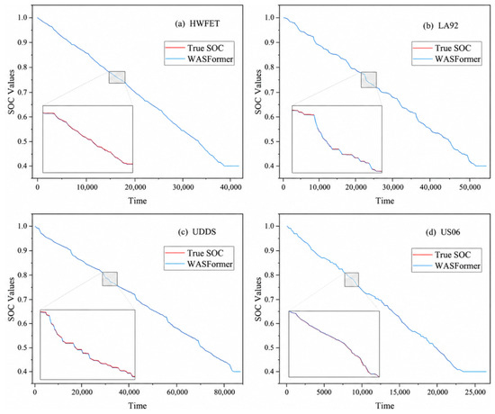
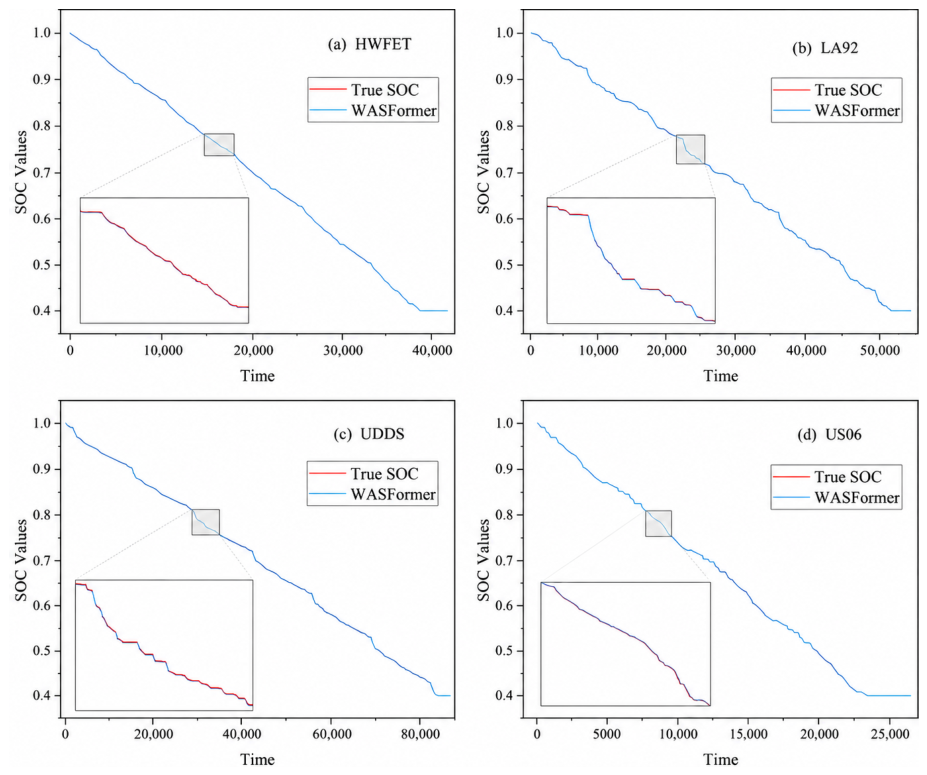
To further evaluate the generalization capability of the WASFormer model, this study conducted tests across four operating condition datasets at temperatures of −20 °C, −10 °C, 0 °C, 10 °C, and 25 °C. The performance metrics of the SOC estimation results are presented in

Table 5. Generalization test results of the WASFormer model.

Operating Conditions	Temperature	MAE	RMSE	MAPE	R2
HWFET	−20 °C	0.025	0.027	0.036	99.99978
	−10 °C	0.015	0.018	0.029	99.99993
	0 °C	0.056	0.057	0.121	99.99945
	10 °C	0.099	0.100	0.254	99.99855
	25 °C	0.167	0.168	0.541	99.99639
UDDS	−20 °C	0.046	0.047	0.070	99.99927
	−10 °C	0.008	0.010	0.014	99.99998
	0 °C	0.042	0.042	0.085	99.99967
	10 °C	0.087	0.087	0.218	99.99886
	25 °C	0.157	0.157	0.246	99.99663
LA92	−20 °C	0.030	0.033	0.044	99.99968
	−10 °C	0.012	0.017	0.022	99.99993
	0 °C	0.051	0.052	0.107	99.99953
	10 °C	0.094	0.096	0.200	99.99838
	25 °C	0.162	0.163	0.417	99.99610
US06	−20 °C	0.027	0.032	0.043	99.99971
	−10 °C	0.054	0.059	0.105	99.99925
	0 °C	0.086	0.089	0.196	99.99870
	10 °C	0.124	0.127	0.264	99.99716
	25 °C	0.188	0.190	0.533	99.99502

. Taking the −20 °C test results as an example, the goodness-of-fit between the estimated SOC values and the actual values, along with the local error curves, are illustrated in Figure 9.

Analysis of Table 5 and Figure 9 clearly shows that under different operating conditions and temperature levels, the SOC estimation error of the WASFormer model generally increases with rising temperature. Overall, regardless of operating condition, the model exhibits relatively high estimation accuracy in low-temperature environments. As temperature rises, corresponding error metrics generally increase. Nevertheless, the model’s R² values remain near 100% across all operating conditions, demonstrating excellent data fitting capability. Specifically, under the HWFET operating condition at −20 °C, the model achieves its lowest SOC estimation error: MAE is only 0.025%, RMSE is 0.027%, MAPE is 0.036%, and R² reaches an exceptionally high 99.99978%. Even under the US06 operating condition at 25 °C, which exhibits the highest estimation error, the model maintains satisfactory accuracy with MAE of 0.188%, RMSE of 0.190%, MAPE of 0.533%, and R² of 99.9502%. In summary, the WASFormer model demonstrates outstanding SOC estimation accuracy and generalization capability across diverse operating conditions and temperatures. The relatively small magnitude of the reported errors is largely due to the characteristics of the dataset: a high sampling frequency of 0.1 s and a large number of samples (over 380,000) provide dense and informative sequences for model training. As a result, prediction errors naturally fall within a small numerical range. Therefore, the main focus of the comparative experiments is to evaluate the relative performance of WASFormer against baseline models, rather than the absolute error magnitude. This emphasizes the effectiveness and generalization capability of the proposed model under diverse operating conditions.

3.3.3. Robustness Analysis

To further evaluate the robustness of the proposed model, an additional noise perturbation experiment is conducted. Specifically, zero-mean Gaussian noise with different standard deviations (σ = 0.01 and σ = 0.1) is injected into the input feature sequences under multiple driving cycles and temperature conditions.

This experiment aims to simulate measurement uncertainties and assess the stability of the model under degraded data quality. The results are summarized in

Table 6. RMSE Results of the WASFormer Model under Different Noise Levels.

Operating Conditions	Temperature	σ = 0	σ = 0.01	σ = 0.1
HWFET	−20 °C	0.027	0.144	0.669
	−10 °C	0.018	0.153	0.402
	0 °C	0.057	0.184	0.838
	10 °C	0.100	0.423	0.964
	25 °C	0.168	0.771	1.137
UDDS	−20 °C	0.047	0.153	0.652
	−10 °C	0.010	0.044	0.383
	0 °C	0.042	0.174	0.482
	10 °C	0.087	0.111	0.637
	25 °C	0.157	0.178	0.921
LA92	−20 °C	0.033	0.056	0.364
	−10 °C	0.017	0.039	0.196
	0 °C	0.052	0.068	0.729
	10 °C	0.096	0.219	0.869
	25 °C	0.163	0.284	0.926
US06	−20 °C	0.032	0.162	0.473
	−10 °C	0.059	0.185	0.672
	0 °C	0.089	0.222	0.810
	10 °C	0.127	0.268	0.824
	25 °C	0.190	0.411	0.948

.

The results in Table 6 show that the RMSE values increase as the noise level rises from σ = 0 to σ = 0.1 across all driving cycles and temperature conditions. This trend is expected, as higher noise levels introduce greater uncertainty in the input features. Under moderate noise (σ = 0.01), the model maintains relatively low error levels, indicating stable performance under realistic measurement perturbations. When the noise level increases to σ = 0.1, the error growth remains gradual rather than abrupt, suggesting that the model does not exhibit instability under noisy conditions. In addition, the model demonstrates consistent behavior across different driving cycles, including HWFET, UDDS, LA92, and US06, as well as across a wide temperature range. This indicates that the model retains its generalization capability under varying operating conditions.

Overall, these results support the robustness of the proposed method against input noise and confirm its stability under different environmental and operational scenarios.

3.3.4. Ablation Study

In this section, an ablation study is conducted on WASFormer to investigate not only the contribution of each component to the overall prediction accuracy, but also its role in addressing key challenges in SOC estimation under complex operating conditions. Specifically, RoPE is intended to enhance temporal positional modeling, the WAS mechanism improves the capture of both local and long-range temporal dependencies, Attention Sinks strengthen the preservation of global contextual information, and Huber Loss increases robustness to outliers and measurement noise. By selectively removing these components, the ablation study helps reveal their individual contributions to SOC estimation performance and provides insight into the design rationale of the proposed framework.

Specifically, we conducted ablation tests on four components—Huber Loss, RoPE, the WAS mechanism, and its Attention Sinks—under the −20 °C condition across various scenarios. The strategies defined are: w/o A (Huber Loss) replaces the loss function with MSE Loss; w/o B (RoPE) uses the WASFormer model with traditional absolute position encoding only; w/o C (WAS) refers to removing the WAS mechanism and replacing it with a multi-head attention mechanism; w/o D (AS) denotes the WAS mechanism with Attention Sinks removed, while other components remain unchanged; Ours (WASFormer) represents the strategy proposed in this study.

Table 7. Ablation study results for each component.

Metrics		Ours	w/o A	w/o B	w/o C	w/o D
HWFET	MAE	0.025	0.056	0.134	0.183	0.155
	RMSE	0.027	0.057	0.164	0.185	0.158
	MAPE	0.036	0.086	0.246	0.276	0.233
	R2	99.99978	99.99905	99.99399	99.98993	99.99263
UDDS	MAE	0.046	0.075	0.024	0.222	0.192
	RMSE	0.047	0.076	0.031	0.223	0.193
	MAPE	0.070	0.115	0.035	0.342	0.293
	R2	99.99927	99.99812	99.99970	99.98373	99.98786
LA92	MAE	0.030	0.063	0.065	0.141	0.117
	RMSE	0.033	0.065	0.074	0.147	0.125
	MAPE	0.044	0.097	0.112	0.203	0.163
	R2	99.99968	99.99874	99.99834	99.99345	99.99527
US06	MAE	0.027	0.029	0.024	0.064	0.068
	RMSE	0.032	0.034	0.035	0.077	0.082
	MAPE	0.043	0.047	0.044	0.112	0.122
	R2	99.99971	99.99967	99.99964	99.99833	99.99811

details the SOC estimation results after ablation of each component.

Ablation study results show that each component of the WASFormer model plays a significant positive role in overall prediction performance. As shown in Table 7, removing the RoPE component generally leads to a decrease in performance; only under the UDDS operating conditions does performance see a slight increase. Under all other operating conditions, removing any single component results in a significant increase in prediction error.

Specifically, replacing the Huber loss with the MSE loss generally resulted in a slight decline in the model’s estimation accuracy. The MAE, RMSE, and MAPE increased by approximately 75%, 67%, and 79%, respectively. Meanwhile, removing RoPE significantly reduced the model’s ability to perceive temporal positions. The average increase in RMSE was 119%, reaching 0.164% under the HWFET operating conditions with the highest error. This indicates that the relative position encoding provided by RoPE plays a crucial role in capturing both short-term and long-term temporal dependencies.

In contrast, the absence of Attention Sinks and the WAS mechanism leads to a more severe decline in prediction performance. Specifically, after removing Attention Sinks, the model’s ability to capture global trends is significantly weakened, with the average MAE and RMSE across the four operating conditions increasing by 316% and 301%, respectively. Notably, under the UDDS operating condition, the MAE and RMSE reached 0.192% and 0.193%, These findings indicate that Attention Sinks play a crucial role in absorbing noise and stabilizing the performance of the WAS mechanism; conversely, when the WAS mechanism is completely removed, the model’s inability to accurately capture both local details and global features results in the most severe decline in prediction accuracy. Overall, MAE increased by an average of 377%, and RMSE rose by approximately 355% on average. The large relative percentage increases are mainly due to the extremely low baseline errors of the full WASFormer model. Because the baseline is near zero, even small absolute changes result in large relative percentages. The increase in prediction error was particularly significant under the UDDS condition, fully demonstrating that the WAS mechanism’s strategy of combining local window attention with Attention Sinks can effectively capture multiscale information ranging from local abrupt changes to global degradation trends, thereby significantly improving the model’s prediction accuracy.

4. Conclusions

In this study, we proposed a SOC estimation strategy for lithium-ion batteries based on the Window Attention Sinks Transformer (WASFormer) model to address the challenges of accurate SOC estimation under multiple operating conditions and a wide temperature range. The model integrates Rotary Positional Encoding (RoPE) and the Window Attention Sinks (WAS) mechanism within the PatchTST architecture, allowing it to capture both local feature variations and global degradation trends. Additionally, Huber Loss and Reversible Instance Normalization (RevIN) were employed to improve robustness against noise and distribution shifts. Furthermore, the Tree-structured Parzen Estimator (TPE) algorithm was used to fine-tune the network hyperparameters, further optimizing the model’s performance.

The model was trained and evaluated using high-resolution (0.1 s) cycling data under multiple driving cycles and temperatures, including HWFET, UDDS, LA92, US06, and NN profiles at −20 °C, −10 °C, 0 °C, 10 °C, and 25 °C. Results demonstrate that WASFormer consistently achieves superior SOC estimation accuracy and strong generalization across diverse operating conditions.

The quantitative improvements over baseline models are clear: the WASFormer model achieves an average RMSE of 0.099%, compared with iTransformer (2.604%), Informer (4.126%), GRU (1.967%), NLiner (0.539%), and DLiner (1.372%). For the US06 scenario at 25 °C, the model shows MAE, RMSE, and MAPE of approximately 0.2%, 0.2%, and 0.6%, respectively, illustrating the estimation performance under the tested condition. The inclusion of the EKF benchmark further demonstrates that the proposed method achieves improved performance compared to conventional model-based approaches under the same operating conditions.

The ablation study highlights the importance of each model component, particularly the WAS mechanism and Attention Sinks, in capturing multi-scale temporal features and mitigating noise. Removing these components leads to noticeable increases in estimation errors, confirming their contribution to accurate SOC prediction.

The WASFormer model is designed to be efficient for real-time inference, as it requires only a forward pass once trained. Its attention-based mechanism allows it to focus on informative signals from voltage, current, temperature, and SOE sequences, providing robustness to measurement noise. In addition, the computational cost analysis demonstrates that the proposed model maintains a favorable balance between estimation accuracy and deployment requirements, with a memory consumption of 1.02 MB, 266,761 parameters, and an inference time of 3.12 s. These characteristics indicate that the model can be deployed for online SOC estimation within practical battery management systems (BMSs), supporting real-time operation in electric vehicles and energy storage systems. Although the present study was conducted using the Panasonic 18650PF dataset, the proposed framework is not inherently restricted to a specific battery type and can be adapted to other commercial batteries through retraining or fine-tuning using data collected from the target battery.

In summary, the WASFormer model provides an efficient and robust approach for SOC estimation in lithium-ion batteries across the examined conditions. Its performance and generalization under the tested datasets indicate potential applicability for battery health management in electric vehicles and energy storage systems. Nevertheless, the present study does not systematically investigate the minimum amount of training data required to achieve satisfactory estimation performance. Future work will focus on data-efficiency analysis and cross-battery transferability to further enhance the practical applicability of the proposed framework.

References

- Falcone, P.M. Sustainable Energy Policies in Developing Countries: A Review of Challenges and Opportunities. Energies 2023, 16, 6682. [Google Scholar] [CrossRef] [Scilit]
- Kostenko, G.; Zaporozhets, A. Transition from Electric Vehicles to Energy Storage: Review on Targeted Lithium-Ion Battery Diagnostics. Energies 2024, 17, 5132. [Google Scholar] [CrossRef] [Scilit]
- Haraz, A.; Abualsaud, K.; Massoud, A. State-of-Health and State-of-Charge Estimation in Electric Vehicles Batteries: A Survey on Machine Learning Approaches. IEEE Access 2024, 12, 158110–158139. [Google Scholar] [CrossRef] [Scilit]
- Tian, Y.; Lai, R.; Li, X.; Xiang, L.; Tian, J. A Combined Method for State-of-Charge Estimation for Lithium-Ion Batteries Using a Long Short-Term Memory Network and an Adaptive Cubature Kalman Filter. Appl. Energy 2020, 265, 114789. [Google Scholar] [CrossRef] [Scilit]
- El Daoudi, S.; Lazrak, L. Comparison between PI-DTC-SPWM and Fuzzy Logic for a Sensorless Asynchronous Motor Drive. Prot. Control Mod. Power Syst. 2021, 6, 34. [Google Scholar] [CrossRef] [Scilit]
- Hosseini, S.A.; Taheri, B.; Abyaneh, H.A.; Razavi, F. Comprehensive Power Swing Detection by Current Signal Modeling and Prediction Using the GMDH Method. Prot. Control Mod. Power Syst. 2021, 6, 15. [Google Scholar] [CrossRef] [Scilit]
- Yang, N.; Zhang, X.; Shang, B.; Li, G. Unbalanced Discharging and Aging Due to Temperature Differences among the Cells in a Lithium-Ion Battery Pack with Parallel Combination. J. Power Sources 2016, 306, 733–741. [Google Scholar] [CrossRef] [Scilit]
- Hannan, M.A.; Lipu, M.S.H.; Hussain, A.; Mohamed, A. A Review of Lithium-Ion Battery State of Charge Estimation and Management System in Electric Vehicle Applications: Challenges and Recommendations. Renew. Sustain. Energy Rev. 2017, 78, 834–854. [Google Scholar] [CrossRef] [Scilit]
- Ren, Z.; Du, C. A Review of Machine Learning State-of-Charge and State-of-Health Estimation Algorithms for Lithium-Ion Batteries. Energy Rep. 2023, 9, 2993–3021. [Google Scholar] [CrossRef] [Scilit]
- Campestrini, C.; Kosch, S.; Jossen, A. Influence of Change in Open Circuit Voltage on the State of Charge Estimation with an Extended Kalman Filter. J. Energy Storage 2017, 12, 149–156. [Google Scholar] [CrossRef] [Scilit]
- Ma, N.; Yin, H.; Wang, K. Prediction of the Remaining Useful Life of Supercapacitors at Different Temperatures Based on Improved Long Short-Term Memory. Energies 2023, 16, 5240. [Google Scholar] [CrossRef] [Scilit]
- Solomon, O.O.; Zheng, W.; Chen, J.; Qiao, Z. State of Charge Estimation of Lithium-Ion Battery Using an Improved Fractional-Order Extended Kalman Filter. J. Energy Storage 2022, 49, 104007. [Google Scholar] [CrossRef] [Scilit]
- Sidorov, D.; Panasetsky, D.; Tomin, N.; Karamov, D.; Zhukov, A.; Muftahov, I.; Dreglea, A.; Liu, F.; Li, Y. Toward Zero-Emission Hybrid AC/DC Power Systems with Renewable Energy Sources and Storages: A Case Study from Lake Baikal Region. Energies 2020, 13, 1226. [Google Scholar] [CrossRef] [Scilit]
- Shu, X.; Li, G.; Zhang, Y.; Shen, S.; Chen, Z.; Liu, Y. Stage of Charge Estimation of Lithium-Ion Battery Packs Based on Improved Cubature Kalman Filter with Long Short-Term Memory Model. IEEE Trans. Transp. Electrif. 2021, 7, 1271–1284. [Google Scholar] [CrossRef] [Scilit]
- Sun, H.; Sun, J.; Zhao, K.; Wang, L.; Wang, K. Data-Driven ICA-Bi-LSTM-Combined Lithium Battery SOH Estimation. Math. Probl. Eng. 2022, 2022, 9645892. [Google Scholar] [CrossRef] [Scilit]
- Li, D.; Wang, L.; Duan, C.; Li, Q.; Wang, K. Temperature Prediction of Lithium-ion Batteries Based on Electrochemical Impedance Spectrum: A Review. Int. J. Energy Res. 2022, 46, 10372–10388. [Google Scholar] [CrossRef] [Scilit]
- Deng, Z.; Hu, X.; Lin, X.; Che, Y.; Xu, L.; Guo, W. Data-Driven State of Charge Estimation for Lithium-Ion Battery Packs Based on Gaussian Process Regression. Energy 2020, 205, 118000. [Google Scholar] [CrossRef] [Scilit]
- Hu, J.N.; Hu, J.J.; Lin, H.B.; Li, X.P.; Jiang, C.L.; Qiu, X.H.; Li, W.S. State-of-Charge Estimation for Battery Management System Using Optimized Support Vector Machine for Regression. J. Power Sources 2014, 269, 682–693. [Google Scholar] [CrossRef] [Scilit]
- Li, C.; Chen, Z.; Cui, J.; Wang, Y.; Zou, F. The Lithium-Ion Battery State-of-Charge Estimation Using Random Forest Regression. In Proceedings of the 2014 Prognostics and System Health Management Conference (PHM-2014 Hunan); IEEE: Zhangjiajie, China, 2014; pp. 336–339. [Google Scholar]
- Fan, T.-E.; Liu, S.-M.; Tang, X.; Qu, B. Simultaneously Estimating Two Battery States by Combining a Long Short-Term Memory Network with an Adaptive Unscented Kalman Filter. J. Energy Storage 2022, 50, 104553. [Google Scholar] [CrossRef] [Scilit]
- Jiao, M.; Wang, D.; Qiu, J. A GRU-RNN Based Momentum Optimized Algorithm for SOC Estimation. J. Power Sources 2020, 459, 228051. [Google Scholar] [CrossRef] [Scilit]
- Hu, C.; Cheng, F.; Ma, L.; Li, B. State of Charge Estimation for Lithium-Ion Batteries Based on TCN-LSTM Neural Networks. J. Electrochem. Soc. 2022, 169, 030544. [Google Scholar] [CrossRef] [Scilit]
- Tian, Y.; Lai, R.; Li, X.; Tian, J. State-of-Charge Estimation for Lithium-Ion Batteries Based on Attentional Sequence-to-Sequence Architecture. J. Energy Storage 2023, 62, 106836. [Google Scholar] [CrossRef] [Scilit]
- Zou, R.; Duan, Y.; Wang, Y.; Pang, J.; Liu, F.; Sheikh, S.R. A Novel Convolutional Informer Network for Deterministic and Probabilistic State-of-Charge Estimation of Lithium-Ion Batteries. J. Energy Storage 2023, 57, 106298. [Google Scholar] [CrossRef] [Scilit]
- Bian, C.; He, H.; Yang, S.; Huang, T. State-of-Charge Sequence Estimation of Lithium-Ion Battery Based on Bidirectional Long Short-Term Memory Encoder-Decoder Architecture. J. Power Sources 2020, 449, 227558. [Google Scholar] [CrossRef] [Scilit]
- Peng, J.; Qian, X.; Xu, X.; Wu, W.; Wang, J. State of Charge Estimation Techniques for Lithium-Ion Batteries: A Review. Energy Technol. 2025, 13, 2500542. [Google Scholar] [CrossRef] [Scilit]
- Barik, S.; Saravanan, B. Recent Developments and Challenges in State-of-Charge Estimation Techniques for Electric Vehicle Batteries: A Review. J. Energy Storage 2024, 100, 113623. [Google Scholar] [CrossRef] [Scilit]
- Lim, B.; Zohren, S. Time-Series Forecasting with Deep Learning: A Survey. Phil. Trans. R. Soc. A 2021, 379, 20200209. [Google Scholar] [CrossRef] [Scilit] [PubMed]
- Kim, T.; Kim, J.; Tae, Y.; Park, C.; Choi, J.-H.; Choo, J. Reversible Instance Normalization for Accurate Time-Series Forecasting against Distribution Shift. In Proceedings of the International Conference on Learning Representations (ICLR 2022), Virtual Event, 25–29 April 2022. [Google Scholar]
- Su, J.; Lu, Y.; Pan, S.; Murtadha, A.; Wen, B.; Liu, Y. RoFormer: Enhanced Transformer with Rotary Position Embedding. Neurocomputing 2024, 568, 127063. [Google Scholar] [CrossRef] [Scilit]
- Press, O.; Smith, N.A.; Lewis, M. Train Short, Test Long: Attention with Linear Biases Enables Input Length Extrapolation. In Proceedings of the International Conference on Learning Representations (ICLR 2022), Virtual Event, 25–29 April 2022. [Google Scholar]
- Huang, L.; Yuan, Y.; Guo, J.; Zhang, C.; Chen, X.; Wang, J. Interlaced Sparse Self-Attention for Semantic Segmentation. arXiv 2019. [Google Scholar] [CrossRef] [Scilit]
- Xu, Y.; Nag, S.; Li, D.; Tian, L.; Barsoum, E. MSWA: Refining Local Attention with Multi-ScaleWindow Attention. arXiv 2025. [Google Scholar] [CrossRef] [Scilit]
- Xiao, G.; Tian, Y.; Chen, B.; Han, S.; Lewis, M. Efficient Streaming Language Models with Attention Sinks. In Proceedings of the International Conference on Learning Representations (ICLR 2024), Vienna, Austria, 7–11 May 2024. [Google Scholar]
- Devlin, J.; Chang, M.-W.; Lee, K.; Toutanova, K. BERT: Pre-training of Deep Bidirectional Transformers for Language Understanding. In Proceedings of the 2019 Conference of the North American Chapter of the Association for Computational Linguistics: Human Language Technologies, Minneapolis, MN, USA, 2–7 June 2019; Association for Computational Linguistics: Minneapolis, MN, USA, 2019; pp. 4171–4186. [Google Scholar] [CrossRef] [Scilit]
- Watanabe, S. Tree-Structured Parzen Estimator: Understanding Its Algorithm Components and Their Roles for Better Empirical Performance. arXiv 2025. [Google Scholar] [CrossRef] [Scilit]
- Liu, Y.; Hu, T.; Zhang, H.; Wu, H.; Wang, S.; Ma, L.; Long, M. iTransformer: Inverted Transformers Are Effective for Time Series Forecasting. In Proceedings of the International Conference on Learning Representations (ICLR 2024), Vienna, Austria, 7–11 May 2024. [Google Scholar]
- Zhou, H.; Zhang, S.; Peng, J.; Zhang, S.; Li, J.; Xiong, H.; Zhang, W. Informer: Beyond Efficient Transformer for Long Sequence Time-Series Forecasting. Proc. AAAI Conf. Artif. Intell. 2021, 35, 11106–11115. [Google Scholar] [CrossRef] [Scilit]
- Cho, K.; van Merriënboer, B.; Gulcehre, C.; Bahdanau, D.; Bougares, F.; Schwenk, H.; Bengio, Y. Learning Phrase Representations Using RNN Encoder–Decoder for Statistical Machine Translation. In Proceedings of the 2014 Conference on Empirical Methods in Natural Language Processing (EMNLP), Doha, Qatar, 25–29 October 2014; Association for Computational Linguistics: Doha, Qatar, 2014; pp. 1724–1734. [Google Scholar] [CrossRef] [Scilit]
- Zeng, A.; Chen, M.; Zhang, L.; Xu, Q. Are Transformers Effective for Time Series Forecasting? Proc. AAAI Conf. Artif. Intell. 2023, 37, 11121–11128. [Google Scholar] [CrossRef] [Scilit]
- Kollmeyer, P. Panasonic 18650PF Li-ion Battery Data; Mendeley Data: Version 1; University of Wisconsin-Madison: Madison, WI, USA, 2018. [Google Scholar] [CrossRef]
Disclaimer/Publisher’s Note: The statements, opinions and data contained in all publications are solely those of the individual author(s) and contributor(s) and not of MDPI and/or the editor(s). MDPI and/or the editor(s) disclaim responsibility for any injury to people or property resulting from any ideas, methods, instructions or products referred to in the content. |
© 2026 by the authors. Licensee MDPI, Basel, Switzerland. This article is an open access article distributed under the terms and conditions of the Creative Commons Attribution (CC BY) license.