Adaptive Generalization in Lithium-Ion Battery RUL Prediction via Synergistic Attention–Residual Networks

Abstract

Accurate prediction of remaining useful life (RUL) for lithium-ion batteries remains a critical yet complex challenge due to highly non-linear degradation dynamics and profound data heterogeneity across varying operational profiles. While convolutional neural networks (CNNs) have shown promise in battery health management, traditional architectures struggle with gradient vanishing in deep feature spaces and lack the adaptive capacity to filter early-cycle noise under diverse degradation conditions. To improve robust RUL estimation across heterogeneous benchmark datasets, this paper proposes a deep learning framework that integrates residual connections with dual-attention mechanisms (ResCNN). Specifically, the residual structures effectively mitigate gradient degradation during the extraction of abstract degradation patterns. Concurrently, a synergistic Squeeze-and-Excitation (SE) and Multi-Head Attention module adaptively calibrates channel-wise feature importance and captures long-range temporal dependencies inherent in complex capacity fade processes. The proposed framework is evaluated under a wide spectrum of degradation conditions and distinct cathode systems (LFP and LCO) using both dataset-specific train/validation/test protocols and strict source-to-target cross-dataset transfer tests. Experimental results demonstrate that ResCNN achieves consistently lower prediction errors than baseline models across the evaluated datasets and maintains positive explanatory power on unseen target datasets without target-domain training. Ablation studies further validate the synergistic contribution of each architectural component toward capturing intrinsic battery aging phenomena.

1. Introduction

1.1. Research Background

Lithium-ion batteries are widely used in electric vehicles, aerospace systems, portable electronics, and grid-scale energy storage because of their high energy density and long cycle life. During repeated cycling, however, batteries undergo capacity degradation until they reach the end-of-life (EoL) threshold. Accurate remaining useful life (RUL) prediction is therefore a central function of battery management systems (BMSs). Reliable RUL estimates can support safer operation, maintenance planning, and life-cycle cost reduction [1,2]. For this reason, lithium-ion battery RUL prediction has become a major problem in battery health management [3].

Early RUL prediction methods often relied on mechanistic degradation models based on electrochemical or physical assumptions. These models can provide interpretable descriptions of aging processes, but they are difficult to parameterize across complex operating conditions [4,5]. Data-driven methods offer a complementary route by learning degradation patterns from historical cycling data without explicitly modeling every internal electrochemical process [6,7]. Their development has moved from traditional machine learning toward deep learning models that can represent nonlinear temporal degradation patterns.

1.2. Related Research Work

Data-driven lithium-ion battery RUL prediction methods analyze historical operating data, including voltage, current, temperature, and capacity trajectories. They learn degradation patterns from these measurements and estimate the remaining cycles before the end-of-life threshold. Earlier studies mainly used handcrafted health indicators with support vector regression, random forests, Gaussian processes, or particle filters [8,9,10,11,12]. These methods can be effective when diagnostic features are carefully selected. However, their performance is often sensitive to feature engineering and to shifts in cycling protocol, chemistry, or temperature.

Deep sequence models have therefore become a major direction in recent battery prognostics. RNNs, LSTMs, and GRUs model capacity degradation as a temporal process and can capture sequential dependencies in cycle data [13,14,15,16]. Several studies further combine recurrent networks with optimized health indicators, metaheuristic hyperparameter search, or uncertainty estimation to improve prediction stability [17,18,19,20]. Nevertheless, recurrent models process sequences sequentially, which can limit their efficiency on long degradation histories. They may also struggle to represent short-term regeneration effects and long-range dependencies at the same time.

CNN-based and temporal convolutional approaches address this issue by extracting local degradation patterns through convolutional filters. In battery RUL prediction, CNNs can learn informative features from charge–discharge curves, voltage–capacity profiles, and capacity decay sequences [21,22,23]. More recent temporal convolutional network (TCN) models use causal or dilated convolutions to enlarge the temporal receptive field while retaining parallelizable training. TCN-LSTM and attention-assisted TCN variants have been reported for SOH and RUL estimation under limited or incomplete cycling data [24,25,26]. These studies show that convolutional sequence models can capture local fluctuation and capacity-regeneration patterns, but they still require mechanisms for selecting the most informative channels and time regions.

Transformer-based models have also attracted increasing attention for RUL prediction. Their self-attention mechanism can directly model long-range temporal dependencies and interactions among degradation features. Recent studies have introduced temporal encodings, denoising autoencoders, or hybrid LSTM–Transformer structures to improve prediction under random charging and discharging conditions [27,28]. These methods are well suited to long sequences, but their performance can depend heavily on data scale and regularization. For battery datasets with limited cells, attention modules must be designed carefully to avoid overfitting and unstable extrapolation.

Another active line of research focuses on transfer learning and domain adaptation. Battery datasets often differ in chemistry, manufacturer, temperature, current profile, and termination criterion. Models trained on one dataset may therefore fail when applied to another. Transfer learning methods reuse representations learned from source cells and update them with limited target-cell data [29]. Domain adaptation methods, including adversarial transfer learning and discrepancy-based alignment, attempt to reduce distribution mismatch between source and target batteries [30,31]. These approaches directly address cross-condition generalization, but they usually require explicit source-target adaptation procedures or at least some target-domain observations.

Recent work has also emphasized uncertainty-aware and physics-informed RUL prediction. Uncertainty-aware methods use Bayesian neural networks, Gaussian processes, particle filters, or prediction intervals to quantify confidence in the estimated RUL [19,32,33]. This is important for maintenance decisions, where an accurate point estimate may still be insufficient. Physics-informed approaches introduce degradation laws, state equations, monotonicity constraints, or electrochemical priors into data-driven models [32,33,34]. These models improve interpretability and can reduce physically implausible predictions. However, they often require reliable physical assumptions or model parameters that may not be available across heterogeneous public datasets.

Overall, recent RUL research has progressed from handcrafted features and recurrent networks toward attention-based, transferable, uncertainty-aware, and physics-guided models. The remaining challenge is to build a model that captures local degradation morphology, long-range temporal dependencies, and variability across battery datasets without requiring a separate adaptation procedure for every new battery group. This motivates the present ResCNN framework, which combines residual convolutional feature extraction with channel-wise and temporal attention mechanisms.

1.3. Limitations of Existing Research and the Focus of This Study

Although recent RUL prediction studies have introduced TCNs, Transformers, transfer learning, uncertainty-aware models, and physics-informed frameworks, several practical challenges remain. First, convolutional feature extractors can encounter gradient degradation when deeper architectures are used to represent complex battery aging patterns. As the number of layers increases, gradients may decay during backpropagation and reduce the effective update of deep parameters. This limitation can restrict the extraction of abstract degradation features. In cross-dataset prediction, the problem becomes more difficult because degradation characteristics vary across chemistries and operating conditions.

Second, many CNN-based models treat feature channels and time steps with limited adaptive weighting during feature extraction. In battery degradation data, informative signals are unevenly distributed across channels and cycle regions. Some temporal segments contain discriminative aging information, whereas others mainly contain noise or redundant variation. Without a feature-selection mechanism, predictions can be influenced by early-cycle noise, local regeneration, or protocol-dependent artifacts.

Third, generalization under heterogeneous battery conditions remains a key barrier to practical use. Electric vehicles and energy storage systems may include batteries from different manufacturers, chemistries, and operating environments. Retraining a separate model for every battery group is often impractical. A useful RUL model should therefore retain predictive value across datasets and operating conditions while making clear where calibration or adaptation is still needed.

To address these issues, this study proposes ResCNN, a deep convolutional model that integrates residual structures with attention mechanisms for lithium-ion battery RUL prediction. The main contributions are as follows:

(1) Inspired by ResNet, residual connections are introduced between convolutional layers to support deeper feature extraction. These connections provide direct information and gradient pathways, helping the model represent abstract degradation patterns while maintaining stable convergence.

(2) A Squeeze-and-Excitation (SE) attention mechanism is embedded to recalibrate feature channels. This module allows ResCNN to emphasize channels that are more informative for RUL prediction and suppress less relevant or noisy responses.

(3) A multi-head attention module is incorporated to capture long-range temporal dependencies from multiple representational subspaces. This design helps the model integrate information from different positions in the degradation sequence.

(4) ResCNN is evaluated on three public datasets using both dataset-specific experiments and strict source-to-target transfer tests. These evaluations assess prediction accuracy, component contribution, and cross-dataset generalization under heterogeneous degradation conditions.

2. Model Building and Methods

2.1. Convolutional Neural Network (CNN)

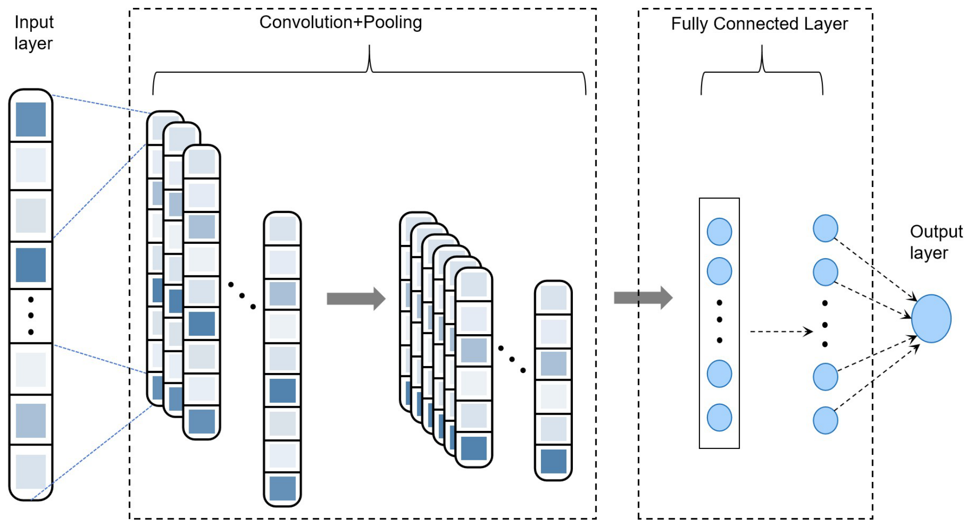
Convolutional neural networks (CNNs) were first developed for image processing and are now widely used for structured data such as time series, text, and video. Their main advantage is the ability to learn local patterns from data through convolutional filters [35,36,37]. A typical CNN contains convolutional layers, pooling layers, and fully connected layers. Convolutional layers extract local spatial or temporal features, pooling layers reduce dimensionality and computational cost, and fully connected layers map the learned features to the final prediction. In battery RUL prediction, CNNs can learn degradation-related patterns from historical cycling data and reduce reliance on handcrafted features [38,39]. The abstract CNN structure is shown in Figure 1.

The convolution layer performs a filtering operation on the input data using a convolution kernel to extract local features. The convolution operation formula is:

$$Y(i,j)=(X\ast W)(i,j)+b$$

(1)

where X is the input data, W is the convolution kernel, b is the bias, and $Y(i,j)$ is the convolution output. The operator ∗ represents convolution. This operation enables the CNN to extract local features from charge–discharge data.

Pooling operations are used to reduce the dimensionality of features and decrease computational load. The formula is:

$$Y(i,j)=\underset{(m,n)\in \mathrm{window}}{max}X(i+m,j+n)$$

(2)

Here, window denotes the size of the pooling window, and $X(i+m,j+n)$ is the input feature value. This operation is performed to reduce the data dimensionality and computational cost.

The formula for the fully connected output layer is:

$$y=W_{2}f(W_{1}f(W_{0}x+b_0)+b_1)+b_2$$

(3)

The fully connected layer flattens the features extracted by the convolutional and pooling layers and maps them to the output through weighted summation. In RUL prediction, this structure allows CNNs to process charge–discharge time-series data and learn temporal degradation patterns.

2.2. Residual Convolution Module

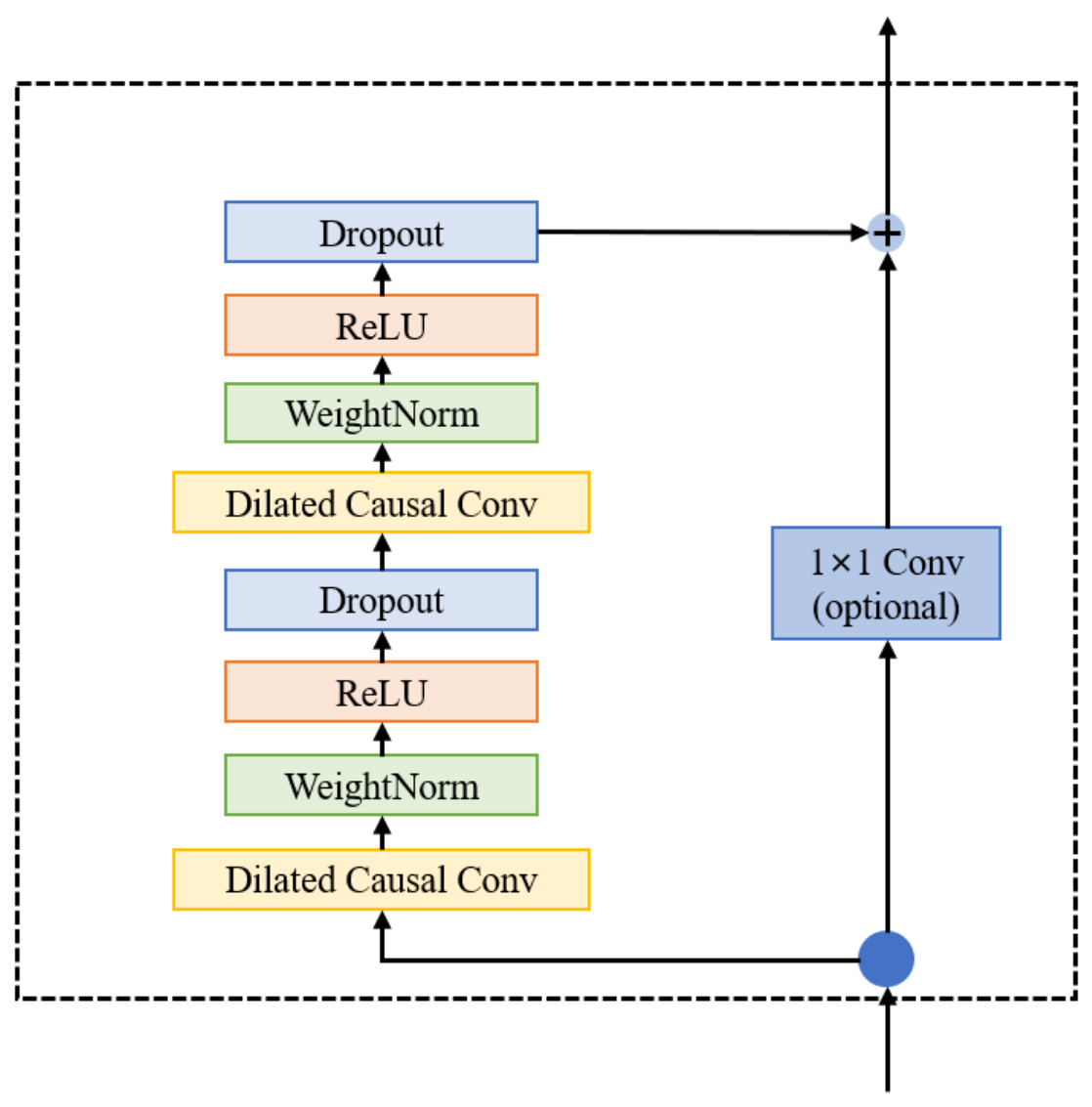
Residual blocks are central components of the ResCNN model. They address gradient degradation in deep CNNs by adding the block input directly to the convolutional output [40]. This shortcut pathway supports backward gradient propagation and allows deeper convolutional features to be trained more stably. A residual block therefore consists of a convolutional transformation and a residual connection. The structure of the residual block is shown in Figure 2.

The mathematical expression for the residual block is:

$$Y_{\mathrm{out}}=F(X,W)+X$$

(4)

The residual-block calculation can be written as:

$$Y_{\mathrm{out}}=\mathrm{ReLU}(\mathrm{Conv}(X,W)+X)$$

(5)

Here, $\mathrm{Conv}$ denotes convolution, $\mathrm{ReLU}$ is the activation function, X is the input, and $Y_{\mathrm{out}}$ is the output after residual addition. In ResCNN, stacked residual blocks process temporal degradation features and help propagate informative signals across layers [41,42,43]. The resulting features are then passed to subsequent modules, including SE attention and multi-head attention.

2.3. SE Attention Mechanism

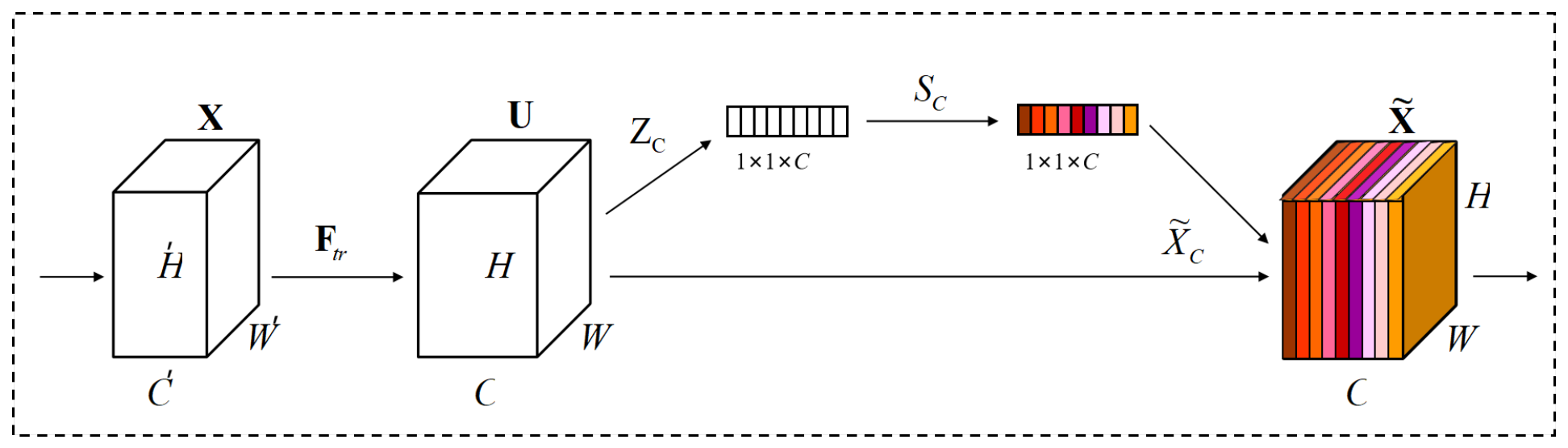
The Squeeze-and-Excitation (SE) mechanism is a channel-wise attention module that assigns adaptive weights to feature channels [44,45]. In ResCNN, SE attention is embedded after the residual blocks to improve channel selection and feature recalibration. This is useful for battery RUL prediction because degradation-related information may be concentrated in a subset of channels, while other channels may contain noise or redundant variation. Channel-level weighting therefore helps the model emphasize degradation-relevant responses [46,47,48]. The SE attention structure is shown in Figure 3.

The SE mechanism contains three stages. During the squeeze stage, global information for each channel is obtained through global average pooling (GAP). The corresponding expression is:

$$z_c={\displaystyle \frac{1}{H\times W}}{\displaystyle \sum _{i=1}^H}{\displaystyle \sum _{j=1}^W}{x}_{ijc}$$

(6)

Here, $x_{ijc}$ denotes the value of the cth channel of the input feature at position $(i,j)$, where H and W represent the height and width of the input feature map, respectively, and $z_c$ is the global information for the cth channel.

The excitation stage learns channel-importance weights through a small fully connected network. The network first reduces the dimensionality of the squeezed descriptor and then generates channel weights using ReLU and sigmoid activations. The corresponding expression is:

$$s_c=\sigma \left(W_2\delta \left(W_1{z}_c\right)\right)$$

(7)

Here, $z_c$ denotes the output of the Squeeze phase, $W_1$ and $W_2$ represent the weights of the fully connected layer, $\delta$ is the ReLU activation function, and $s_c$ is the activation weight for channel c.

During the reweighting stage, the generated excitation weight $s_c$ is multiplied with the corresponding original feature channel. This operation produces recalibrated channel features. The corresponding expression is:

$${\tilde{X}}_c=s_c·X_c$$

(8)

Here, $X_c$ denotes the feature of the cth channel, $s_c$ represents the corresponding excitation weight, and ${\tilde{X}}_c$ indicates the re-calibrated feature.

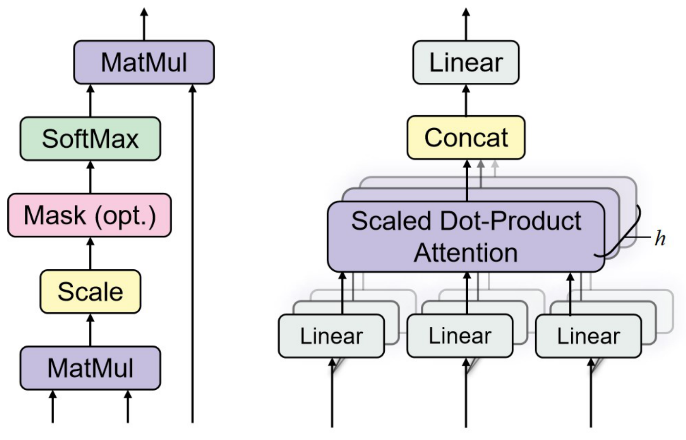
2.4. Multi-Head Attention Module

The multi-head attention module models dependencies among different positions in a sequence by using multiple attention heads in parallel [49]. Each head can attend to a different representational subspace. In ResCNN, multi-head attention complements residual convolution and SE attention by capturing long-range temporal interactions in battery degradation features.

The core operation of multi-head attention is to compute weighted sums of value vectors using attention weights derived from query-key similarity. In RUL prediction, this mechanism helps the model integrate degradation information across cycle count, voltage response, and load-related variation. It also allows the model to attend to different degradation patterns in parallel, such as capacity decay and local regeneration behavior [50,51]. The multi-head attention structure is shown in Figure 4.

Input features are projected into query, key, and value vectors. Each attention head computes similarity scores between queries and keys, normalizes the scores with a softmax function, and applies the resulting weights to the value vectors. The calculation is:

$$\mathrm{Attention}\mathrm{Score}={\displaystyle \frac{Q{K}^T}{\sqrt{d_k}}}$$

(9)

$$\mathrm{Attention}\mathrm{Weights}=\mathrm{Softmax}\left({\displaystyle \frac{Q{K}^T}{\sqrt{d_k}}}\right)$$

(10)

$${\mathrm{Output}}_h=\mathrm{Attention}\mathrm{Weights}·V$$

(11)

$${\mathrm{Output}}_{\mathrm{multihead}}=\mathrm{Concat}\left({\mathrm{Output}}_1,{\mathrm{Output}}_2,\dots ,{\mathrm{Output}}_h\right)W_O$$

(12)

Here, Q is the query matrix, K is the key matrix, V is the value matrix, $d_k$ is the key dimension, h is the number of heads, and $W_O$ is the output projection matrix. The head outputs are concatenated and linearly transformed before being passed to the next layer. This operation fuses multiple attention subspaces into a richer temporal representation.

2.5. ResCNN Model Architecture

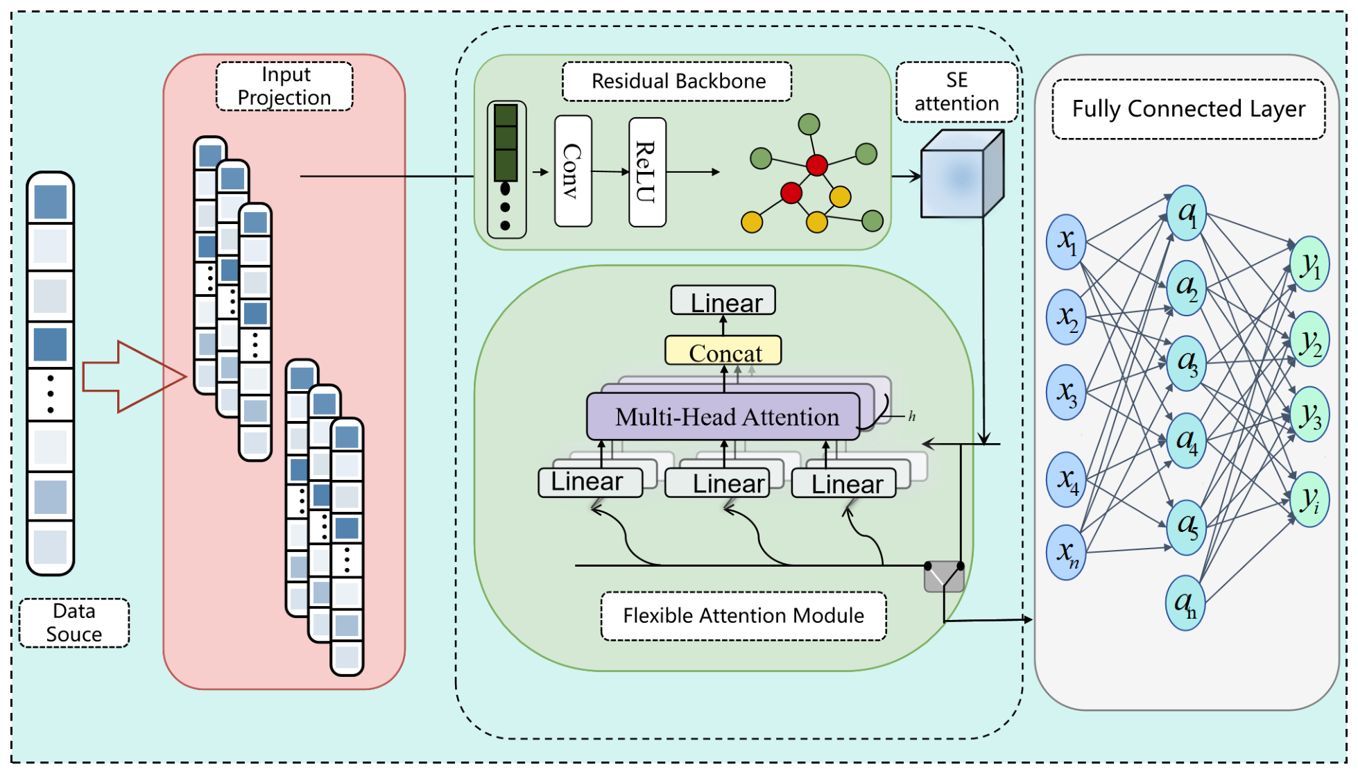
ResCNN combines CNN-based local feature extraction with residual connections, SE channel attention, and multi-head temporal attention. The resulting architecture is designed to capture local degradation morphology, channel-level importance, and long-range temporal dependencies for battery RUL prediction. The ResCNN structure is shown in Figure 5.

A complete layer-by-layer implementation specification of ResCNN is provided in Appendix A,

Table A1. Compact layer-by-layer implementation specification of the proposed ResCNN architecture.

Module	Layer-by-Layer Operation	Output Size	Implementation Details
Input	Voltage–capacity feature matrix	$1\times 100\times 1000$	One channel; first 100 cycles; 1000 interpolated voltage–capacity points.
Projection	Conv2D → BatchNorm → ReLU	$16\times 100\times 1000$	Conv2D $1\to 16$, $3\times 3$, stride 1, padding 1, bias disabled.
Residual block 1	BN-ReLU-Conv → Dropout → BN-ReLU-Conv → SE → residual addition → AvgPool	$32\times 50\times 500$	Main path $16\to 32\to 32$; skip path $1\times 1$ Conv $16\to 32$; pool $2\times 2$/2.
Residual block 2	BN-ReLU-Conv → Dropout → BN-ReLU-Conv → SE → residual addition → AvgPool	$64\times 25\times 250$	Main path $32\to 64\to 64$; skip path $1\times 1$ Conv $32\to 64$; pool $2\times 2$/2.
Residual block 3	BN-ReLU-Conv → Dropout → BN-ReLU-Conv → SE → pooled residual addition → AvgPool	$64\times 12\times 125$	Main path $64\to 64\to 64$; pooled identity skip; pool $2\times 2$/2.
Attention	SE channel recalibration → multi-head self-attention over compressed spatial tokens	$64\times 12\times 125$	SE reduction ratio 8; attention preserves the residual feature-map size after token compression and interpolation.
Global pooling	Adaptive average pooling ‖ adaptive max pooling → concatenation	128	Concatenates two 64-dimensional global descriptors.
Regression head	Linear → LayerNorm → ReLU → Dropout → Linear → LayerNorm → ReLU → Dropout → Linear	1	Fully connected mapping $128\to 64\to 32\to 1$ for scalar RUL prediction.

Note: The reproducible ResCNN configuration used in this study is: base channels = 64, dropout = 0.15, convolution kernel size = 3, SE reduction ratio = 8, number of residual blocks = 3, optimizer = Adam, and RUL output dimension = 1. Output sizes follow the channel-first convention $C\times H\times W$.

.

3. Data Sources and Experimental Settings

3.1. Data Introduction

This study used three publicly available lithium-ion battery cycling datasets for model training and evaluation: MATR [52,53,54], HUST [55,56], and CALCE [57,58]. Together, these datasets cover LFP and LCO cathode systems and include different operating conditions. They therefore provide a heterogeneous benchmark for evaluating ResCNN under multiple degradation scenarios. Detailed descriptions of the three datasets follow.

The MATR dataset, derived from the MIT–Stanford–Toyota Research Institute fast-charging battery datasets and standardized in BatteryML, is widely used for lithium-ion battery state-of-health and RUL studies. It contains 180 LFP/graphite cells with a rated capacity of 1.1 Ah. The cells were aged under multiple cycling rates and temperature conditions, including constant-current/constant-voltage (CC–CV) charging protocols. Its broad lifetime distribution and diverse degradation curves make it suitable for training data-driven models.

The HUST dataset, provided by Huazhong University of Science and Technology, contains degradation measurements from 77 LFP/graphite cells with a rated capacity of 1.1 Ah. It covers different discharge rates, ambient temperatures, and cycling strategies. Compared with MATR, HUST contains longer lifetime scales and nonlinear degradation patterns under more varied operating conditions. These characteristics make it useful for testing model robustness across protocols.

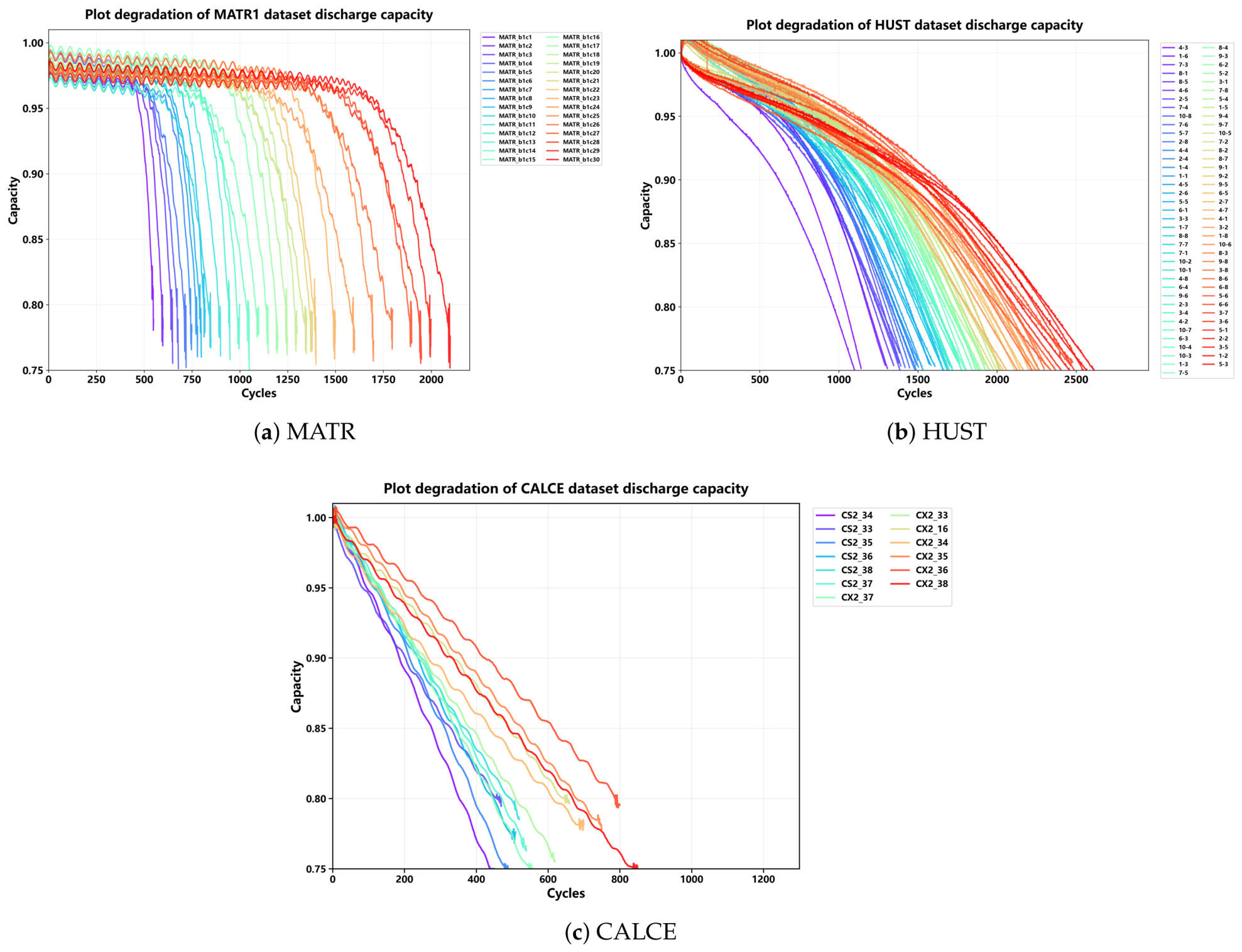
The CALCE dataset originates from the Center for Advanced Life Cycle Engineering (CALCE) at the University of Maryland. It contains 13 LCO/graphite cells with a rated capacity of 1.1 Ah tested under standardized protocols. Although the dataset is small, its controlled experimental conditions make it a useful benchmark for assessing prediction behavior under a different cathode system. The discharge capacity of each dataset as a function of cycle number is shown in Figure 6.

As shown in Figure 6, the datasets differ in degradation trajectory morphology, lifetime scale, and sample consistency. MATR exhibits a dispersed lifetime distribution, phased degradation behavior, and pronounced cell-to-cell variation. Some samples show rapid degradation during the early or middle cycling stages. In contrast, HUST contains longer overall lifetimes and more concentrated capacity-decay curves.

Unlike the two LFP datasets, CALCE uses an LCO cathode system and shows a different degradation pattern. Its cells have shorter lifetimes, more monotonic nonlinear capacity decline, and smaller fluctuations among samples.

Table 1. Summary of battery chemistries and experimental conditions of the datasets.

Dataset	Battery Count	Chemistry	Capacity (Ah)	Voltage Range (V)	Average RUL
MATR	180	LFP/Graphite	1.1	2.0–3.6	1009 ± 698
HUST	77	LFP/Graphite	1.1	2.0–3.6	1899 ± 389
CALCE	13	LCO/Graphite	1.1	2.7–4.2	566 ± 106

summarizes the battery counts, chemistries, voltage ranges, and lifetime distributions of the datasets. Even within the LFP cathode system, different experimental conditions and acquisition protocols produce distinct degradation distributions. The additional chemistry difference between LFP and LCO further changes the statistical properties and temporal structure of capacity profiles. These differences motivate the evaluation of whether ResCNN can maintain stable performance across heterogeneous datasets.

3.2. Experiment Settings

The ResCNN implementation used 64 base channels, three residual convolutional blocks, a $3\times 3$ convolution kernel, ReLU activation, a dropout rate of 0.15, an SE reduction ratio of 8, and the Adam optimizer for parameter updates. The model receives one 100 × 1000 voltage–capacity feature matrix as input and outputs one scalar RUL prediction. A complete layer-by-layer architecture is provided in Appendix A to support reproducibility.

Before feature extraction, all raw battery cycling records were processed using the same deterministic screening procedure. For each dataset, records were first ordered by battery identifier and cycle index. Cycles lacking complete voltage, current, time, or discharge-capacity measurements were excluded. Records with non-physical values, including negative time increments, non-positive discharge capacity, or voltage values outside the dataset-specific nominal ranges in Table 1, were also removed. Duplicate cycle indices and incomplete charge–discharge records were discarded so that each retained observation corresponded to one valid cycle.

During feature extraction, the VoltageCapacityMatrixFeatureExtractor was used to extract voltage–capacity curve features. A window-level prediction record denotes one RUL label paired with one feature matrix generated from an eligible observation window of a battery. Each record was converted into a 100 × 1000 two-dimensional feature matrix. The differential baseline cycle was set to the 9th cycle, and the maximum cycle index was set to 99, corresponding to the first 100 cycles. Precomputed Qdlin (discharge capacity) was used for feature extraction. To improve numerical stability and comparability, the feature matrix was normalized by Z-score scaling. Because RUL values showed a long-tailed distribution, labels were first logarithmically transformed and then Z-score normalized.

After raw-data screening, the remaining voltage–capacity trajectories were converted into a unified input representation. Voltage–capacity curves were aligned to a common voltage–capacity grid and interpolated to form fixed-size feature matrices. In the cross-dataset experiments, target-domain records were not used to estimate cleaning, normalization, or feature-scaling parameters. Deterministic integrity checks were applied before the battery-level split. Normalization statistics for model input scaling were fitted only on the corresponding training subset or source training domain to avoid information leakage.

All dataset splits were performed at the battery level to avoid information leakage. MATR was divided into training, validation, and test sets at an 8:1:1 ratio, yielding approximately 18 held-out test batteries. HUST was divided at a 7:1.5:1.5 ratio, yielding approximately 12 held-out test batteries after integer rounding. After the battery-level split, window-level prediction records were generated only within their assigned subset. No record derived from a validation or test battery was used for model training. Because CALCE contains only 13 batteries, leave-one-out cross-validation was used. Each iteration reserved one battery for testing and used the remaining batteries for training.

To assess source-to-target cross-dataset generalization, three zero-target-training transfer experiments were designed. In the first experiment, ResCNN was trained on the MATR source-domain training split and evaluated directly on all HUST batteries (MATR → HUST). In the second experiment, the direction was reversed, with training on HUST and direct evaluation on MATR (HUST → MATR). These tests assess transferability between two LFP/graphite datasets with different cycling protocols and degradation distributions. In the third experiment, ResCNN was trained on the two LFP datasets (MATR + HUST) and evaluated directly on the LCO/graphite CALCE dataset (LFP → CALCE). No CALCE cell was used for training or fine-tuning. For all cross-dataset tests, the feature extractor, label definition, normalization strategy, and evaluation metrics were kept consistent with the within-dataset experiments. Feature and label normalization parameters were fitted only on the source training domain and applied unchanged to the target domain. No target-domain battery was used for training, validation, hyperparameter selection, normalization-parameter fitting, or model selection.

For the comparative experiments, the same training strategy, preprocessing pipeline, and evaluation metrics were applied to all baseline models. The baselines included Baseline CNN(a standard convolutional neural network without residual connections or attention mechanisms), LSTM (Long Short-Term Memory network), SVR (Support Vector Regression), and Random Forest.

To analyze the contribution of each ResCNN component, ablation experiments were performed using the configurations shown in

Table 2. ResCNN Ablation Experiment Design.

Experiment	Residual Connection	SE Attention	Multi-Head Attention	Pre-Activation
Baseline CNN	×	×	×	×
CNN + Residual	✓	×	×	×
CNN + Residual + SE	✓	✓	×	×
ResCNN (Full Model)	✓	✓	✓	✓

Note: “✓” indicates that the corresponding module is included, whereas “×” indicates its exclusion.

.

3.3. Experimental Implementation Environment

All experiments were implemented in Python 3.10.13 with PyTorch 2.1.2. GPU acceleration was enabled through CUDA 11.8. Model training, validation, testing, ablation experiments, and baseline comparisons were conducted under the same software environment, preprocessing pipeline, dataset splitting strategy, and evaluation metrics.

The experiments were run on a workstation equipped with an Intel Core i9-12900K CPU operating at 3.20 GHz, 64 GB RAM, and an NVIDIA GeForce RTX 3090 GPU with 24 GB memory. This configuration was used for model training and for the non-embedded inference-time measurements reported in

Table 3. Performance comparison between ResCNN and baseline models across different datasets, including RMSE, R², computational efficiency, and statistical significance. The reported inference time is a single-sample forward-pass latency measured under the same non-embedded experimental environment for all models.

Model	MATR RMSE	HUST RMSE	CALCE RMSE	Average RMSE	Average R2	Training Time (s)	Inference Time (ms/Sample)	Parameter Count
SVR	142.5	456.3	68.5	222.4	0.721	350	0.52	1.9 M
Random Forest	128.7	423.8	62.8	205.1	0.759	400	0.60	2.0 M
LSTM	122.4	412.5	58.9	197.9	0.780	900	1.10	2.3 M
CNN	116.3	398.5	54.7	189.8	0.813	820	0.85	2.1 M
ResNet	110.8	378.9	51.2	180.3	0.836	960	1.05	2.5 M
ResCNN	107.8 *	365.3 *	48.3 **	173.8 **	0.877 **	990	1.15	2.8 M

Note: * and ** indicate statistically significant improvements of ResCNN based on paired absolute prediction errors from the same held-out records. Adjusted p values were obtained using two-sided Wilcoxon signed-rank tests with Holm–Bonferroni correction, as described in Section 3.4. * denotes p < 0.05 and ** denotes p < 0.01. For deployment interpretation, the parameter count gives an approximate weight-memory requirement of 11.2 MB for ResCNN under 32-bit floating-point storage (2.8 M parameters × 4 bytes), excluding intermediate activations, runtime libraries, and feature-buffer memory.

. These hardware details support reproducibility and clarify that the reported runtime values reflect the experimental computing platform rather than deployment on embedded BMS hardware.

3.4. Evaluation Metrics

Three regression metrics were used to evaluate battery RUL prediction performance.

(1) Root mean square error (RMSE) measures the square-root average of squared prediction errors. Lower RMSE indicates better prediction performance. It is defined as:

$$\mathrm{RMSE}=\sqrt{{\displaystyle \frac{1}{n}}\sum _{i=1}^n{(y_i-{\widehat{y}}_i)}^2}$$

(13)

(2) Mean absolute error (MAE) measures the average absolute prediction error. Lower MAE indicates better prediction performance. It is defined as:

$$\mathrm{MAE}={\displaystyle \frac{1}{n}}{\displaystyle \sum _{i=1}^n}|y_i-{\widehat{y}}_i|$$

(14)

(3) The coefficient of determination (R²) measures the proportion of target variability explained by the model. Values closer to 1 indicate better fit. Negative values can occur when a model performs worse than predicting the target mean, especially under severe cross-dataset distribution shift. It is defined as:

$${\mathrm{R}}^2=1-{\displaystyle \frac{{\sum }_{i=1}^n{(y_i-{\widehat{y}}_i)}^2}{{\sum }_{i=1}^n{(y_i-\overline{y})}^2}}$$

(15)

Here, n denotes the number of evaluated window-level prediction records, $y_i$ is the true RUL value of the ith record, and ${\widehat{y}}_i$ is the predicted RUL value. For MATR and HUST, this record-level count differs from the number of independent test batteries because the split was conducted at the battery level before record generation. $\overline{y}$ is the mean of the true RUL values.

Statistical significance was assessed using the same held-out prediction records used to calculate the regression metrics. For each dataset and model comparison, absolute prediction errors were paired by evaluation record. Two-sided Wilcoxon signed-rank tests were then used to test whether paired error distributions differed. This non-parametric paired test was selected because normality of the error distributions was not assumed. A statistically significant result was reported as an improvement only when ResCNN also had a lower median absolute error than the comparison model. In Table 3, ResCNN was compared with CNN and with the best-performing non-ResCNN baseline on the same test records. When multiple comparisons were made within a table, p values were adjusted using the Holm–Bonferroni procedure. Statistical annotations therefore indicate adjusted p values, with * denoting $p<0.05$ and ** denoting $p<0.01$.

4. Results and Analysis

4.1. Multi-Dataset Performance Evaluation

Table 3 compares ResCNN with benchmark models on the MATR, HUST, and CALCE datasets. Traditional machine learning models (SVR and Random Forest) showed lower computational overhead, but they produced larger prediction errors than the deep learning models. CNN and LSTM provided a balanced trade-off between accuracy and stability, while ResNet further reduced the prediction error through residual feature extraction.

The proposed ResCNN achieved the lowest RMSE values across all three datasets and the best average R² among the evaluated models. This result indicates stable multi-dataset prediction behavior under different battery systems and operating conditions. The improvement is consistent with the role of residual structures and attention mechanisms in preserving deep features and emphasizing degradation-relevant information.

These results are consistent with recent peer-reviewed studies showing that hybrid sequence models, attention mechanisms, and Transformer variants can improve lithium-ion battery RUL prediction by jointly modeling local degradation fluctuations and long-range temporal dependencies [50,51,59]. CNN–RNN and CNN–BiLSTM variants have been used to combine local feature extraction with sequential modeling, whereas TCN-based hybrids and dual-attention networks emphasize local temporal morphology, feature selection, and degradation-stage sensitivity [24,39,60]. Transformer-based studies further show the value of self-attention for early prediction, random charging and discharging conditions, uncertainty quantification, and patch-level temporal representation [61,62]. Because published studies often use different feature definitions, train/test splits, prediction starting points, and battery datasets, direct numerical ranking across papers is not fully comparable. Therefore, the main comparative value of Table 3 lies in the controlled same-protocol comparison among baseline models and ResCNN across three heterogeneous datasets.

Beyond prediction accuracy, Table 3 reports training duration, parameter count, and single-sample inference time under the same experimental environment. SVR and Random Forest had lower computational overhead during training and inference, while CNN and LSTM showed comparable efficiency. ResNet and ResCNN required slightly higher training costs because of their larger structural complexity and parameter scales. ResCNN achieved a measured single-sample forward-pass latency of 1.15 ms in the non-embedded benchmark, compared with 0.85 ms for CNN and 1.05 ms for ResNet. Thus, the added residual and attention modules introduced only a limited latency increase in the evaluated software environment. These values should be interpreted as relative computational indicators, not direct evidence of deployability on embedded BMS hardware.

For embedded deployment, memory and runtime constraints must be considered explicitly. ResCNN contains 2.8 M parameters, corresponding to approximately 11.2 MB of weight memory with 32-bit floating-point storage. Additional memory is required for intermediate activations, input feature buffers, preprocessing, and inference runtime support. Direct deployment on low-resource microcontrollers may therefore require model compression, fixed-point quantization, memory reuse, or hardware acceleration. Because this study did not benchmark the model on a specific automotive-grade BMS processor, microcontroller, or edge accelerator, we restrict the deployment claim to computational feasibility under the reported experimental setting. Target-specific embedded profiling remains necessary before practical online BMS deployment.

4.2. Strict Cross-Dataset Generalization

To distinguish multi-dataset robustness from true source-to-target transfer, we evaluated ResCNN under three strict cross-dataset protocols in which no target-domain cell was used for training or fine-tuning. The results are summarized in

Table 4. Strict source-to-target cross-dataset evaluation of ResCNN without target-domain training or fine-tuning.

Transfer Protocol	Source Chemistry	Target Chemistry	RMSE/MAE (Cycles)	R2
MATR → HUST	LFP/graphite	LFP/graphite	369.9/300.2	0.875
HUST → MATR	LFP/graphite	LFP/graphite	109.2/83.1	0.915
LFP → CALCE	LFP/graphite	LCO/graphite	50.6/38.5	0.831

Note: MATR → HUST and HUST → MATR were evaluated by applying the source-domain-trained model directly to all target-domain batteries. LFP → CALCE used MATR + HUST as the source domain and CALCE as the held-out target domain. Normalization parameters were fitted only on the source training data and then applied unchanged to the target domain. RMSE, MAE, and R² were calculated over the generated target-domain window-level prediction records. The positive R² values indicate that the source-trained model retained explanatory power on unseen target-domain batteries under zero-target-training evaluation.

. These experiments are intentionally more difficult than the within-dataset evaluations in Table 3, because the model must transfer representations across different degradation distributions, cycling protocols, lifetime ranges, and, in the LFP → CALCE case, cathode chemistry.

The cross-dataset results support the ability of ResCNN to transfer learned degradation representations to unseen target datasets without target-domain training or fine-tuning. In the two LFP/graphite transfer settings, MATR → HUST and HUST → MATR achieved RMSE values of 369.9 and 109.2 cycles, with R² values of 0.875 and 0.915, respectively. These results indicate that the model retained predictive accuracy across different cycling protocols, lifetime scales, and degradation morphologies. Such shifts are widely recognized as major sources of performance loss in transfer and time-varying degradation studies [21,22,31]. Compared with the corresponding within-dataset RMSE values in Table 3, MATR → HUST remained close to the HUST same-dataset result (365.3 cycles), and HUST → MATR remained close to the MATR same-dataset result (107.8 cycles). The LFP → CALCE experiment further tested cross-chemistry transfer from LFP/graphite source datasets to the LCO/graphite CALCE target dataset. This setting achieved an RMSE of 50.6 cycles and an R² of 0.831. Although cross-chemistry transfer is more difficult than transfer within the same nominal chemistry, the RMSE was close to the CALCE same-dataset result (48.3 cycles). The positive R² indicates meaningful target-domain explanatory power under a strict zero-target-training protocol. These findings support the adaptive cross-dataset generalization claim while also indicating that target-domain calibration or adaptation may further improve deployment performance.

This zero-target-training setting differs from recent transfer-learning and domain-adaptation studies that explicitly use target-domain observations or distribution-alignment losses to reduce source-target mismatch [21,22,29,31]. Such methods are highly relevant for deployment preparation because they can adapt a source model to a new battery population. In contrast, the present cross-dataset test evaluates whether the residual-attention representation retains predictive value before any target-domain adaptation is introduced. The positive R² values therefore provide a stricter baseline for generalization, while the remaining cross-chemistry gap indicates where physics-informed constraints, domain adaptation, or target-domain calibration may be beneficial [33,34].

4.3. Ablation Study Analysis

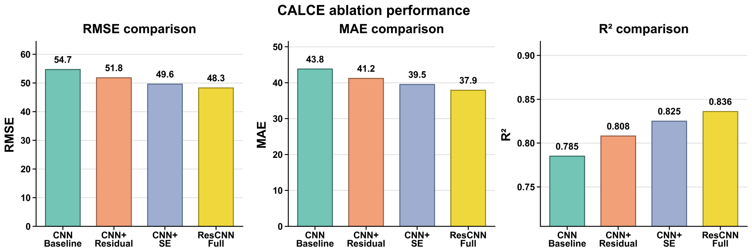
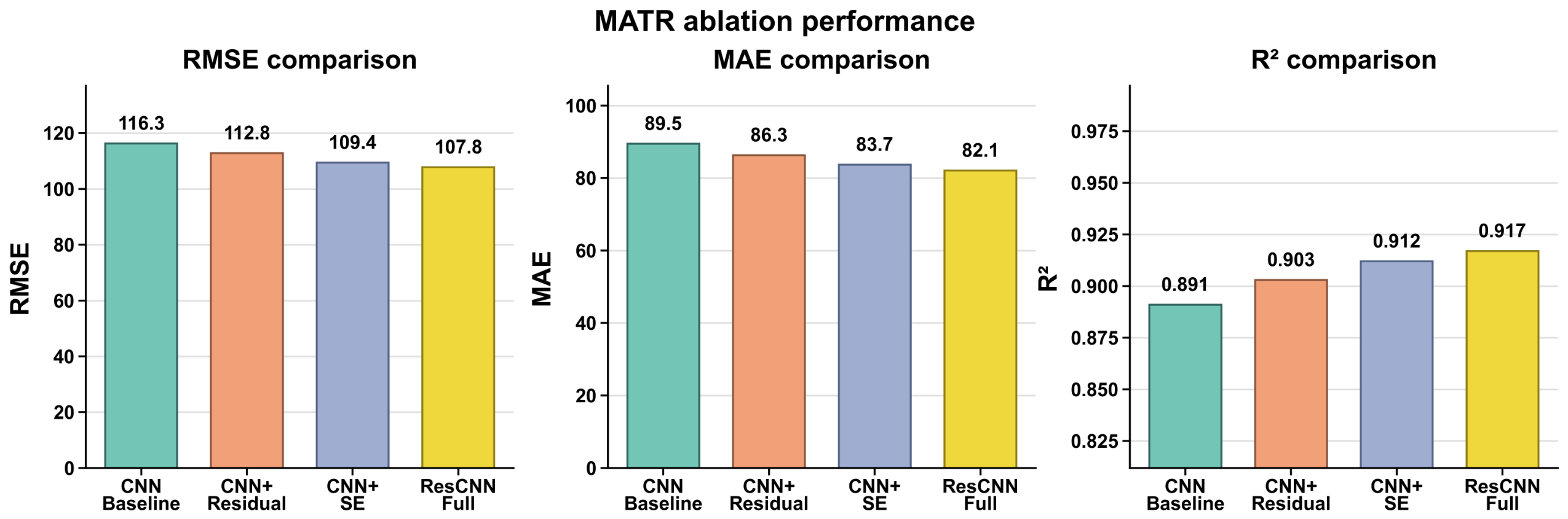
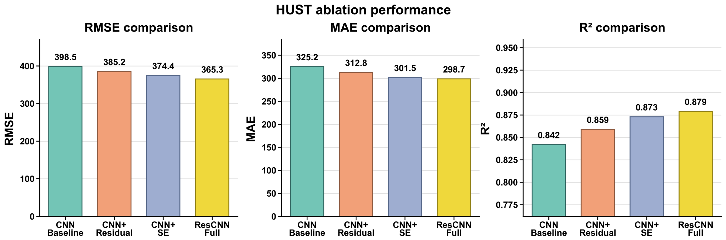
To evaluate the contribution of each ResCNN module, ablation experiments were conducted by progressively adding model components. The configurations ranged from a baseline CNN to the full ResCNN model. Their performance was compared across the MATR (Figure 7), HUST (Figure 8), and CALCE (Figure 9) datasets to quantify the effect of each component.

To quantify the marginal contribution of each module, performance gains were calculated across configurations.

Table 5. Comparative Study of RMSE Ablation for ResCNN Components Across Different Datasets.

Dataset	Model Configuration	RMSE (Cycles)	Improvement (%)
MATR	CNN Baseline	116.3	–
	+ Residual Connection	112.8	+2.9
	+ SE Attention	109.4	+3.2
	Full ResCNN	107.8 **	+7.2 **
HUST	CNN Baseline	398.5	–
	+ Residual Connection	385.2	+3.3
	+ SE Attention	374.4	+3.5
	Full ResCNN	365.3 **	+8.3 **
CALCE	CNN Baseline	54.7	–
	+ Residual Connection	51.8	+2.8
	+ SE Attention	49.6	+3.4
	Full ResCNN	48.3 **	+7.2 **
Average	Full ResCNN	173.8 **	+7.5 **

Note: ** indicates that the full ResCNN model achieves a statistically significant performance improvement compared with the reduced configurations based on paired absolute prediction errors from the same held-out records. Adjusted p values were obtained using two-sided Wilcoxon signed-rank tests with Holm–Bonferroni correction, as described in Section 3.4. The improvement percentage is calculated relative to the CNN baseline.

reports the RMSE reduction associated with each component.

Table 5 shows the ablation results for different model configurations on MATR, HUST, and CALCE. The baseline CNN was used as the reference, and residual connections, SE attention, and multi-head attention were added progressively.

Across all three datasets, introducing residual connections alone reduced prediction errors, lowering RMSE to 112.8, 385.2, and 51.8 cycles, respectively. Adding SE attention further reduced RMSE to 109.4, 374.4, and 49.6 cycles. These results indicate that channel recalibration provides additional performance gains across datasets.

The full ResCNN model achieved the lowest RMSE across all datasets, with values of 107.8, 365.3, and 48.3 cycles on MATR, HUST, and CALCE, respectively. These values correspond to improvement rates of 7.2%, 8.3%, and 7.2% relative to the CNN baseline. The paired Wilcoxon signed-rank tests described in Section 3.4 showed that the full model improved significantly over the reduced configurations after correction ($p<0.01$).

The ablation trend also agrees with recent RUL studies in which residual, convolutional, recurrent, attention-based, and expert-mixture components contribute complementary functions rather than acting as isolated accuracy boosters [26,59,61]. In the present model, residual connections improve deep feature propagation, SE attention recalibrates degradation-relevant channels, and multi-head attention captures temporal interactions across different representational subspaces. This component-level interpretation helps explain why the full ResCNN outperforms reduced configurations across datasets with different degradation morphologies.

On average, ResCNN achieved an RMSE of 173.8 cycles and an improvement rate of 7.5%, indicating consistent gains across the evaluated datasets.

4.4. Predictive Performance Testing

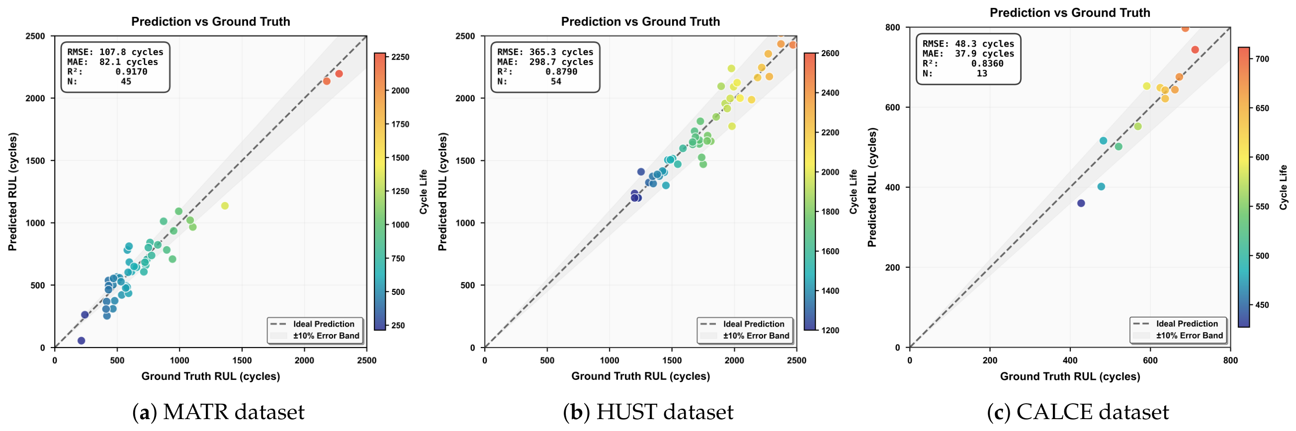
Figure 10 compares ResCNN predictions with the corresponding ground-truth RUL values across the three datasets.

Figure 10 shows the comparison between predicted and ground-truth RUL values obtained by ResCNN on MATR, HUST, and CALCE. Overall, the predicted values followed the ground-truth trend across all datasets, indicating stable prediction behavior under heterogeneous degradation conditions. The plotted N values refer to evaluated window-level prediction records. They should not be interpreted as independent battery counts, because MATR and HUST were split at the battery level before record generation.

On CALCE (N = 13), the predicted values were closely distributed around the ideal diagonal line despite the limited sample size and shorter lifespan range. For HUST, approximately 12 independent batteries were held out for testing, and these batteries produced 54 plotted prediction records. ResCNN maintained a strong correspondence between predicted and actual RUL values over a range of 1200–2600 cycles. For MATR, approximately 18 independent batteries were held out for testing, and these batteries produced 45 plotted prediction records. MATR covered the broadest RUL span (200–2300 cycles) and showed more diverse degradation states. Nevertheless, the predicted values remained aligned with the ground truth across the evaluated protocols.

To quantify within-dataset variation beyond the scatter plots,

Table 6. Sample-level error statistics of ResCNN on the test samples of each dataset.

Dataset	No. of Test Batteries	No. of Prediction Records	Median AE	IQR Width of AE	Max AE
MATR	18	45	72.4	67.3	276.3
HUST	12	54	281.5	224.4	812.6
CALCE	13	13	34.7	29.9	96.5

Note: AE denotes absolute prediction error in cycles. The IQR width is calculated as the difference between the third and first quartiles (Q3–Q1). Sample-level statistics were calculated from the evaluated prediction records shown in Figure 10.

reports sample-level absolute-error statistics for the evaluated prediction records. The HUST dataset shows the largest dispersion, with a median AE of 281.5 cycles, an IQR width of 224.4 cycles, and a maximum AE of 812.6 cycles. This wider spread is consistent with the longer lifetime scale of HUST batteries and the nonlinear degradation patterns observed under diverse operating conditions. Recent studies on uncertainty-aware prediction, two-phase aging, small-sample augmentation, and time-varying degradation also report that regeneration behavior, weak early degradation information, and distribution shifts can produce uneven sample-level prediction errors [22,40]. MATR shows a lower median AE of 72.4 cycles and a smaller IQR width of 67.3 cycles, but its maximum AE of 276.3 cycles indicates that atypical degradation trajectories can still produce larger errors. CALCE exhibits the smallest median AE, IQR width, and maximum AE, partly because its lifetime range is shorter and its testing protocol is more standardized. Overall, larger sample-level errors are mainly associated with cells whose degradation trajectory, lifetime scale, or local regeneration behavior deviates from the dominant patterns represented in the training data.

Quantitatively, the coefficient of determination (R²) exceeded 0.83 for all three datasets, with an average value of 0.877. The MAE-to-RMSE ratios remained within a relatively narrow range (0.75–0.82), indicating a balanced error distribution without pronounced systematic bias. These results support the robustness of ResCNN in multi-dataset RUL prediction evaluation across different chemistries, lifespan distributions, and record counts.

4.5. Training Process Analysis

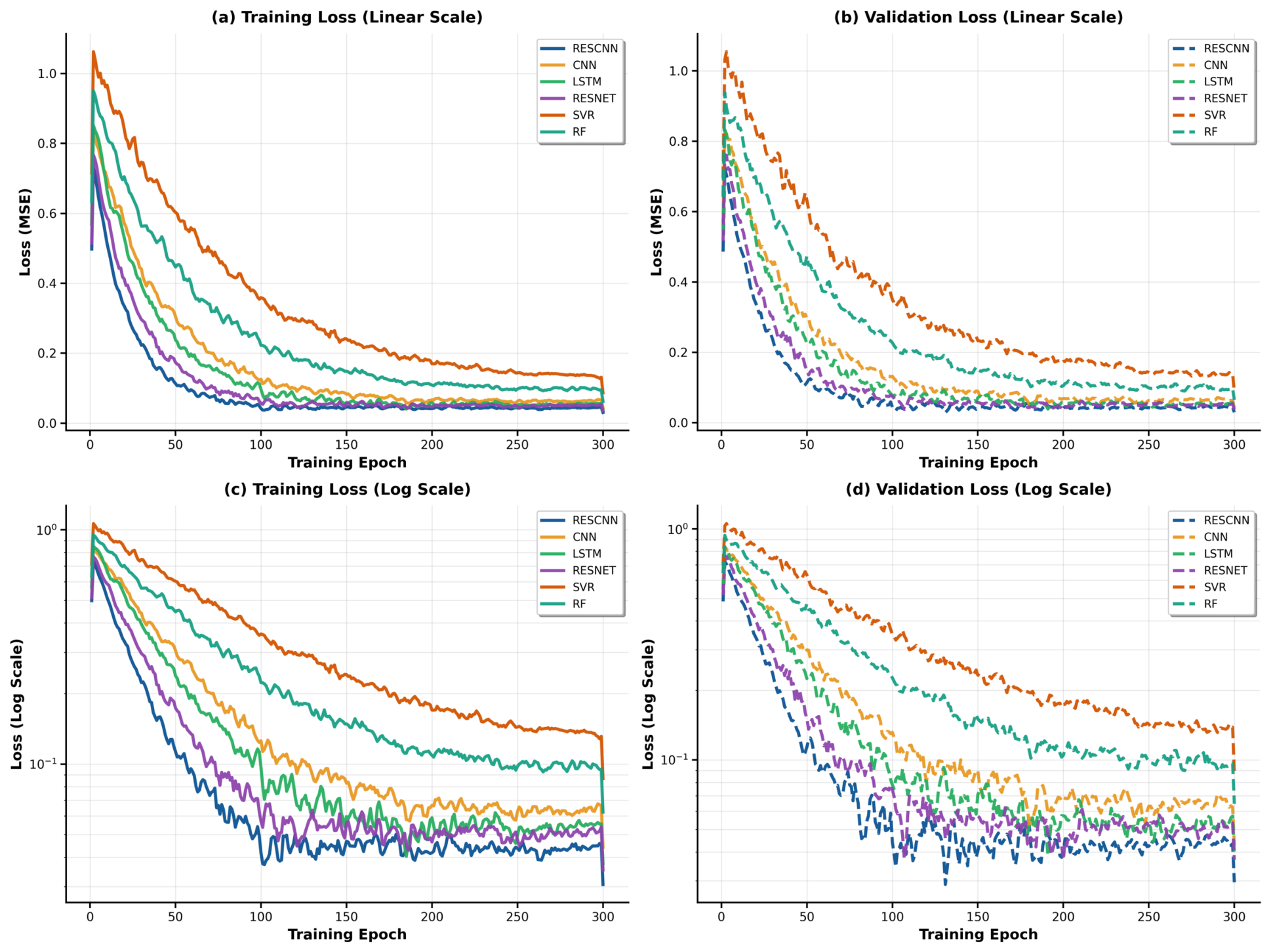
To evaluate the learning behavior and optimization stability of the proposed framework, the training trajectories of all competing models were systematically monitored throughout the learning phase. The continuous variations of both training and validation losses over 300 epochs are visually illustrated in Figure 11.

Figure 11 displays the training and validation loss curves for the six comparison models. Under both linear and logarithmic coordinate scales, it is consistently observable that the training and validation losses of all deep learning architectures exhibit a sharp downward trajectory during the initial training phase. This rapid decline demonstrates their remarkable efficiency in capturing abstract temporal degradation patterns.

To quantitatively evaluate the precise optimization limits and computational efficiency across different architectural configurations, key numerical tracking indicators were extracted from the training logs. The statistical records regarding the convergence velocities and final stabilized loss boundaries are summarized in

Table 7. Comparison of Convergence Performance Across Models: Convergence Periods During Training, Final Loss, and Training–Validation Gap.

Model	90% Convergence Epochs	Final Loss	Training–Validation Gap
ResCNN	45	0.045	<3%
ResNet	58	0.052	5%
LSTM	68	0.055	7%
CNN	72	0.065	9%
Random Forest	95	0.095	11%
SVR	118	0.120	14%

.

Table 7 shows that the deep learning models converged substantially faster than the traditional machine learning baselines. Specifically, ResCNN stabilized after merely 45 epochs, representing a 37.5% acceleration in convergence speed compared with the baseline CNN, and a speedup of over 70% relative to traditional shallow estimators. Furthermore, its final validation loss reached 0.045, which is approximately 30% lower than that of the standard CNN and 60–65% lower than the traditional machine learning approaches. ResCNN also exhibited a smooth optimization profile and the minimum training–validation gap, underscoring its stable evaluation performance within the same dataset. In contrast, the baseline CNN suffered from a 9% generalization gap, while the traditional machine learning methods exceeded 10%. During the training process, the validation loss was monitored after each epoch to dynamically assess convergence quality and detect potential overfitting or divergence between training and validation behaviors. No dataset-specific early-stopping criteria were introduced for the small-sample CALCE domain; thus, all candidate models were executed and evaluated under identical training and validation monitoring protocols to ensure a fair comparison.

To further investigate the potential risks of overfitting, the structural sensitivity of ResCNN to dropout regularization constraints was analyzed. The trade-offs between prediction errors and regularization intensity under varying dropout rates are organized in

Table 8. Sensitivity analysis of dropout regularization for ResCNN.

Dropout Rate	MATR RMSE	HUST RMSE	CALCE RMSE	Training–Validation Gap
0.00	114.6	386.8	52.5	8.7%
0.10	109.1	371.6	49.2	4.1%
0.15	107.8	365.3	48.3	2.5%
0.30	112.7	379.4	51.1	1.8%

Note: The dropout rate of 0.15 was used in the final ResCNN configuration. The training–validation gap was calculated from the final training and validation losses. A smaller gap at a high dropout rate does not necessarily indicate better prediction performance, because excessive dropout may lead to underfitting.

.

As interpreted from the sensitivity records, completely removing the dropout layers (dropout rate = 0.00) expanded the training–validation gap to 8.7% and induced higher RMSE values across all three benchmark domains. This manifestation implies a heightened risk of feature co-adaptation. Conversely, implementing a moderate dropout rate simultaneously mitigated prediction errors and narrowed the divergence between the training and validation subsets. The optimized configuration utilizing a dropout rate of 0.15 successfully achieved the lowest RMSE metrics across the MATR, HUST, and CALCE datasets while constraining the structural divergence below 3%. Although increasing the dropout rate to 0.30 further compressed the generalization gap to 1.8%, it led to an evident inflation of RMSE values across all domains. This degradation pattern suggests that excessive regularization over-suppresses the representational capacity of the network, resulting in underfitting. The trend is consistent with recent RUL studies that use dropout, denoising, or data augmentation to improve robustness under noisy measurements, limited data, or weak early-cycle degradation information [26,59].

Particular caution is required when assessing overfitting on the small-sample CALCE dataset, which contains only 13 independent battery cells. To eliminate split-dependent verification bias, a battery-level leave-one-out cross-validation protocol was adopted for the CALCE domain, as detailed in Section 3.2. Each iteration strictly isolated one individual battery as the independent testing target and assigned the remaining cells for training, thereby preventing individual cycle records from the same physical cell from simultaneously appearing in both the training and testing sets. The low median absolute error (AE) and narrow interquartile range (IQR) width reported in Table 6, paired with the dropout sensitivity profiles in Table 8, confirm that the model maintains commendable stability under this strict evaluation protocol. Nevertheless, given the limited sample size of the CALCE dataset, these numerical responses should be interpreted as supportive validation of the model’s cross-domain transferability rather than absolute evidence of ultimate deployment robustness in uncalibrated field environments.

Together, the convergence curves, small training–validation gap, dropout sensitivity analysis, battery-level evaluation protocol, and cross-dataset tests support the generalization robustness of ResCNN. Residual connections provide direct gradient pathways, attention mechanisms highlight degradation-relevant features, and the selected dropout rate reduces co-adaptation without suppressing useful feature learning.

5. Conclusions

This study proposed ResCNN, a residual convolutional network with SE channel attention and multi-head temporal attention, for lithium-ion battery RUL prediction under heterogeneous degradation conditions. The model was evaluated on three public datasets (MATR, HUST, and CALCE) using both dataset-specific experiments and strict source-to-target transfer protocols.

The multi-dataset results showed that ResCNN achieved lower RMSE and higher average R² than the evaluated traditional machine learning and deep learning baselines. The ablation analysis indicated that residual connections, SE attention, and multi-head attention contributed complementary gains. Residual connections supported stable deep feature extraction, SE attention recalibrated degradation-relevant channels, and multi-head attention captured temporal interactions across different representational subspaces. Strict transfer experiments further showed positive R² values for MATR → HUST, HUST → MATR, and LFP → CALCE transfer, with values of 0.875, 0.915, and 0.831, respectively. These results support the claim that the learned residual-attention representation retains predictive value across datasets without target-domain training or fine-tuning, although cross-chemistry deployment remains more challenging and may require calibration or adaptation.

From an engineering perspective, ResCNN showed a favorable accuracy–efficiency trade-off in the evaluated non-embedded environment. The model achieved 1.15 ms single-sample forward-pass latency and used 2.8M parameters, corresponding to approximately 11.2 MB of weight memory with 32-bit floating-point storage. These measurements indicate computational tractability for further deployment investigation. They do not, however, establish readiness for online operation in production BMS hardware. Practical embedded implementation would require target-specific profiling of latency, peak memory, power consumption, numerical precision, feature-buffer management, and integration with the BMS sampling and diagnostic schedule. Techniques such as pruning, quantization, operator fusion, and incremental updating may be needed to meet low-resource processor constraints.

Practical Deployment Challenges

Several practical risks must be addressed before applying ResCNN in real-world battery management systems. First, field batteries operate under dynamic current profiles, variable temperatures, intermittent rest periods, and user-specific charging behavior. These conditions can shift voltage–capacity patterns away from those represented in public laboratory datasets. Second, battery packs introduce additional inconsistency among cells, including cell-to-cell capacity variation, temperature gradients, balancing effects, and module-level electrical coupling. A model trained on single-cell datasets may therefore require pack-level calibration before deployment. Third, sensor noise, missing records, sampling-rate mismatch, and long-term data drift can affect feature extraction and reduce prediction reliability.

A practical transfer preparation workflow should therefore include several steps. Before deployment, a small target-domain calibration set should be collected under the intended operating conditions and used to check feature distributions, RUL-label definitions, voltage ranges, and normalization parameters. The source-trained model should then be evaluated on target cells or packs without using future-cycle information. If a marked performance drop is observed, lightweight transfer learning, domain calibration, or periodic model updating may be required. During online use, prediction uncertainty, input-distribution drift, and abnormal sensor patterns should be monitored so that unreliable RUL estimates can be flagged instead of being used directly for maintenance decisions. These steps are needed to bridge benchmark-level validation and dependable BMS deployment.

In summary, ResCNN provides a data-driven framework that balances prediction accuracy, cross-dataset robustness, and computational cost in the evaluated benchmark setting. The strict cross-dataset tests support the adaptive generalization claim by showing that source-trained models retained meaningful predictive accuracy on unseen target datasets with different lifetime distributions, cycling protocols, and battery chemistries. Future work should further investigate cross-chemistry calibration, uncertainty estimation, and target-specific embedded profiling before field deployment.

References

1. Zhang, W.; Pranav, R.; Wang, R.; Lee, C.; Zeng, J.; Cho, M.; Shim, J. Lithium-Ion Battery Life Prediction Using Deep Transfer Learning. Batteries 2024, 10, 434. [Google Scholar] [CrossRef]
2. Wang, Z.; Shangguan, W.; Peng, C.; Cai, B. Similarity based remaining useful life prediction for lithium-ion battery under small sample situation based on data augmentation. Eksploat. Niezawodność 2024, 26, 175585. [Google Scholar]
3. Chen, C.; Wei, J.; Li, Z. Remaining useful life prediction for lithium-ion batteries based on a hybrid deep learning model. Processes 2023, 11, 2333. [Google Scholar] [CrossRef]
4. Yuliani, A.R.; Pardede, H.F.; Ramdan, A.; Zilvan, V.; Yuwana, R.S.; Amri, M.F.; Kusumo, R.B.S.; Pramanik, S. Robust remaining useful life prediction of lithium-ion battery with convolutional denoising autoencoder. J. Mechatron. Electr. Power Veh. Technol. 2024, 15, 93–104. [Google Scholar] [CrossRef]
5. Wang, M.; Xiang, G.; Cui, L.; Zhang, Q.; Chen, J. Remaining useful life distribution prediction framework for lithium-ion battery fused prior knowledge and monitoring data. Meas. Sci. Technol. 2023, 34, 125108. [Google Scholar] [CrossRef]
6. Schaeffer, J.; Galuppini, G.; Rhyu, J.; Asinger, P.A.; Droop, R.; Findeisen, R.; Braatz, R.D. Cycle life prediction for lithium-ion batteries: Machine learning and more. In Proceedings of the 2024 American Control Conference (ACC); IEEE: Piscataway, NJ, USA, 2024; pp. 763–768. [Google Scholar]
7. Madani, S.S.; Ziebert, C.; Vahdatkhah, P.; Sadrnezhaad, S.K. Recent progress of deep learning methods for health monitoring of lithium-ion batteries. Batteries 2024, 10, 204. [Google Scholar] [CrossRef]
8. Yang, N.; Hofmann, H.; Sun, J.; Song, Z. Remaining useful life prediction of lithium-ion batteries with limited degradation history using random forest. IEEE Trans. Transp. Electrif. 2023, 10, 5049–5060. [Google Scholar] [CrossRef]
9. Jafari, S.; Byun, Y.C. Optimizing battery RUL prediction of lithium-ion batteries based on Harris hawk optimization approach using random forest and LightGBM. IEEE Access 2023, 11, 87034–87046. [Google Scholar] [CrossRef]
10. Umayal, R.; Darapaneni, N.; Aditya, V.; Paduri, A.R. Machine learning based remaining useful life prediction of lithium-ion batteries in electric vehicle battery management system. In Proceedings of the 2023 International Conference on Communication, Security and Artificial Intelligence (ICCSAI); IEEE: Piscataway, NJ, USA, 2023; pp. 547–551. [Google Scholar]
11. Chen, L.; Zhang, Y.; Zheng, Y.; Li, X.; Zheng, X. Remaining useful life prediction of lithium-ion battery with optimal input sequence selection and error compensation. Neurocomputing 2020, 414, 245–254. [Google Scholar] [CrossRef]
12. Jia, J.; Liang, J.; Shi, Y.; Wen, J.; Pang, X.; Zeng, J. SOH and RUL prediction of lithium-ion batteries based on Gaussian process regression with indirect health indicators. Energies 2020, 13, 375. [Google Scholar] [CrossRef]
13. Li, H.; Chen, C. Lithium-ion battery SOH prediction based on multi-dimensional features and multi-model feature selector. Energy 2025, 331, 136844. [Google Scholar] [CrossRef]
14. Li, H.; Chen, C.; Wei, J.; Chen, Z.; Lei, G.; Wu, L. State of health (soh) estimation of lithium-ion batteries based on abc-bigru. Electronics 2024, 13, 1675. [Google Scholar] [CrossRef]
15. Zhang, S.; Li, Y.; Zhao, D.; Cui, Z.; Zhang, Q. Remaining Useful Life Prediction of a Lithium-Ion Battery Based on AE and Modified Transformer. In Proceedings of the 2023 China Automation Congress (CAC); IEEE: Piscataway, NJ, USA, 2023; pp. 6216–6221. [Google Scholar]
16. He, Z.; Wang, H.; Xiang, J.; Chen, C. Enhancing the Sustainability of Underground Battery Storage: A Robust SOC Estimation Model Against Thermal Variations for Green Energy Systems. J. Geo-Energy Environ. 2025, 1, 88–95. [Google Scholar] [CrossRef]
17. Wang, H.; Li, H.; He, Z.; Chen, X.; Liu, H.; Chen, C. A linear-complexity deep learning framework for efficient battery State of Health estimation in resource-constrained systems. Eng. Appl. Artif. Intell. 2026, 181, 115420. [Google Scholar] [CrossRef]
18. Zraibi, B.; Mansouri, M. Improving Lithium-Ion Battery Reliability Through Neural Network Remaining Useful Life Prediction. IAES Int. J. Artif. Intell. 2025, 14, 83. [Google Scholar] [CrossRef]
19. Reza, M.; Hannan, M.; Mansor, M.; Ker, P.J.; Tiong, S.K.; Hossain, M. Gravitational search algorithm based LSTM deep neural network for battery capacity and remaining useful life prediction with uncertainty. IEEE Trans. Ind. Appl. 2024, 60, 9171–9183. [Google Scholar] [CrossRef]
20. Zhang, Z.; Liu, P.; Ge, W.; Lai, Y. Remaining useful life prediction of lithium-ion battery based on new health factor in long short-term memory network. In Proceedings of the 2023 7th International Conference on Deep Learning Technologies; ACM: New York, NY, USA, 2023; pp. 103–108. [Google Scholar]
21. Li, Z.; Li, J.; Wang, X.; Zhang, C.; Nie, L. Remaining useful life prediction of lithium-ion battery based on AConvST-LSTM-Net-TL. Phys. Scr. 2025, 100, 026010. [Google Scholar]
22. Chen, Z.; Wang, Z.; Wu, W.; Xia, T.; Pan, E. Neural Representation-Based Wiener Process with Meta-Learning for Battery RUL Prediction Under Time-Varying Degradation Rate. IEEE Trans. Instrum. Meas. 2025, 74, 1004313. [Google Scholar]
23. Zhao, J.; Zhu, Y.; Zhang, B.; Liu, M.; Wang, J.; Liu, C.; Hao, X. Review of state estimation and remaining useful life prediction methods for lithium–ion batteries. Sustainability 2023, 15, 5014. [Google Scholar] [CrossRef]
24. Li, C.; Han, X.; Zhang, Q.; Li, M.; Rao, Z.; Liao, W.; Liu, X.; Liu, X.; Li, G. State-of-health and remaining-useful-life estimations of lithium-ion battery based on temporal convolutional network-long short-term memory. J. Energy Storage 2023, 74, 109498. [Google Scholar] [CrossRef]
25. Zhou, D.; Wang, B. Battery health prognosis using improved temporal convolutional network modeling. J. Energy Storage 2022, 51, 104480. [Google Scholar] [CrossRef]
26. Fei, Z.; Zhang, Z.; Yang, F.; Tsui, K.L. A deep attention-assisted and memory-augmented temporal convolutional network based model for rapid lithium-ion battery remaining useful life predictions with limited data. J. Energy Storage 2023, 62, 106903. [Google Scholar] [CrossRef]
27. Song, W.; Wu, D.; Shen, W.; Boulet, B. A Remaining Useful Life Prediction Method for Lithium-ion Battery Based on Temporal Transformer Network. Procedia Comput. Sci. 2023, 217, 1830–1838. [Google Scholar] [CrossRef]
28. Zhang, W.; Jia, J.; Pang, X.; Wen, J.; Shi, Y.; Zeng, J. An Improved Transformer Model for Remaining Useful Life Prediction of Lithium-Ion Batteries under Random Charging and Discharging. Electronics 2024, 13, 1423. [Google Scholar] [CrossRef]
29. Che, Y.; Deng, Z.; Lin, X.; Hu, L.; Hu, X. Predictive Battery Health Management with Transfer Learning and Online Model Correction. IEEE Trans. Veh. Technol. 2021, 70, 1269–1277. [Google Scholar] [CrossRef]
30. Ye, Z.; Yu, J. State-of-Health Estimation for Lithium-Ion Batteries Using Domain Adversarial Transfer Learning. IEEE Trans. Power Electron. 2022, 37, 3528–3543. [Google Scholar] [CrossRef]
31. Tran, K.; Huynh, B.; Le, T.; Pham, L.; Nguyen, V.R.; Tran Anh, D.; Trinh, H.C. HybridoNet-Adapt: A domain-adapted framework for accurate lithium-ion battery RUL prediction. PLoS ONE 2025, 20, e0335066. [Google Scholar] [CrossRef] [PubMed]
32. Najera-Flores, D.A.; Hu, Z.; Chadha, M.; Todd, M.D. A Physics-Constrained Bayesian Neural Network for Battery Remaining Useful Life Prediction. Appl. Math. Model. 2023, 122, 42–59. [Google Scholar] [CrossRef]
33. Nascimento, R.G.; Viana, F.A.C.; Corbetta, M.; Kulkarni, C.S. A framework for Li-ion battery prognosis based on hybrid Bayesian physics-informed neural networks. Sci. Rep. 2023, 13, 13856. [Google Scholar] [CrossRef] [PubMed]
34. Wang, F.; Zhai, Z.; Zhao, Z.; Di, Y.; Kang, B.; Yang, X.; Xie, X.; Deng, Y. Physics-informed neural network for lithium-ion battery degradation stable modeling and prognosis. Nat. Commun. 2024, 15, 4332. [Google Scholar] [CrossRef] [PubMed]
35. Ashwin, T.; Chung, Y.M.; Wang, J. Capacity fade modelling of lithium-ion battery under cyclic loading conditions. J. Power Sources 2016, 328, 586–598. [Google Scholar] [CrossRef]
36. Prasad, G.K.; Rahn, C.D. Model based identification of aging parameters in lithium ion batteries. J. Power Sources 2013, 232, 79–85. [Google Scholar] [CrossRef]
37. Virkar, A.V. A model for degradation of electrochemical devices based on linear non-equilibrium thermodynamics and its application to lithium ion batteries. J. Power Sources 2011, 196, 5970–5984. [Google Scholar] [CrossRef]
38. Zhuang, Z.; Li, Y.; Yang, T. Remaining Useful Life Prediction of Lithium-Ion Battery Based on AUKF and CNN-BiLSTM. In Proceedings of the 2024 IEEE 13th Data Driven Control and Learning Systems Conference (DDCLS); IEEE: Piscataway, NJ, USA, 2024; pp. 13–18. [Google Scholar]
39. Lv, K.; Ma, Z.; Bao, C.; Liu, G. Indirect prediction of lithium-ion battery RUL based on CEEMDAN and CNN-BiGRU. Energies 2024, 17, 1704. [Google Scholar] [CrossRef]
40. Ma, W.; Zhu, H.; Wu, J.; Zhang, S. Deep learning-based remaining useful life prediction of lithium-ion battery considering two-phase aging process. J. Electrochem. Soc. 2024, 171, 120529. [Google Scholar]
41. Liu, J.; Chen, Z. Remaining useful life prediction of lithium-ion batteries based on health indicator and Gaussian process regression model. IEEE Access 2019, 7, 39474–39484. [Google Scholar] [CrossRef]
42. Jiang, B.; Dai, H.; Wei, X.; Jiang, Z. Multi-kernel relevance vector machine with parameter optimization for cycling aging prediction of lithium-ion batteries. IEEE J. Emerg. Sel. Top. Power Electron. 2021, 11, 175–186. [Google Scholar]
43. Wang, Z.; Ma, Q.; Guo, Y. Remaining useful life prediction of lithium-ion batteries based on deep learning and soft sensing. In Proceedings of the Actuators; MDPI: Basel, Switzerland, 2021; Volume 10, p. 234. [Google Scholar]
44. Wu, L.; Guo, W.; Tang, Y.; Sun, Y.; Qin, T. Remaining useful life prediction of lithium-ion batteries based on neural network and adaptive unscented kalman filter. Electronics 2024, 13, 2619. [Google Scholar] [CrossRef]
45. Chen, Z.; Xu, H.; Wei, Y.; Huang, C. Remaining useful life prediction method of lithium-ion battery Based on KPCA-IVMD-SE-DNN. J. Phys. Conf. Ser. 2024, 2741, 012073. [Google Scholar] [CrossRef]
46. Liu, J.; Cheng, K.; Jin, H.; Wu, Z. An image captioning algorithm based on combination attention mechanism. Electronics 2022, 11, 1397. [Google Scholar] [CrossRef]
47. Wang, D.; Xiang, S.; Zhou, Y.; Mu, J.; Zhou, H.; Irampaye, R. Multiple-attention mechanism network for semantic segmentation. Sensors 2022, 22, 4477. [Google Scholar] [CrossRef] [PubMed]
48. Liu, J.; Yang, J.; Liu, K.; Xu, L. Ocean current prediction using the weighted pure attention mechanism. J. Mar. Sci. Eng. 2022, 10, 592. [Google Scholar] [CrossRef]
49. Zhao, L.; Song, S.; Wang, P.; Wang, C.; Wang, J.; Guo, M. A MLP-Mixer and mixture of expert model for remaining useful life prediction of lithium-ion batteries. Front. Comput. Sci. 2024, 18, 185329. [Google Scholar]
50. Li, L.; Li, Y.; Mao, R.; Li, L.; Hua, W.; Zhang, J. Remaining useful life prediction for lithium-ion batteries with a hybrid model based on TCN-GRU-DNN and dual attention mechanism. IEEE Trans. Transp. Electrif. 2023, 9, 4726–4740. [Google Scholar]
51. Wang, T.; Ma, Z.; Zou, S. Remaining useful life prediction of lithium-ion batteries: A temporal and differential guided dual attention neural network. IEEE Trans. Energy Convers. 2023, 39, 757–771. [Google Scholar] [CrossRef]
52. Severson, K.A.; Attia, P.M.; Jin, N.; Perkins, N.; Jiang, B.; Yang, Z.; Chen, M.H.; Aykol, M.; Herring, P.K.; Fraggedakis, D.; et al. Data-driven prediction of battery cycle life before capacity degradation. Nat. Energy 2019, 4, 383–391. [Google Scholar] [CrossRef]
53. Attia, P.M.; Grover, A.; Jin, N.; Severson, K.A.; Markov, T.M.; Liao, Y.H.; Chen, M.H.; Cheong, B.; Perkins, N.; Yang, Z.; et al. Closed-loop optimization of fast-charging protocols for batteries with machine learning. Nature 2020, 578, 397–402. [Google Scholar] [CrossRef] [PubMed]
54. Zhang, H.; Gui, X.; Zheng, S.; Lu, Z.; Li, Y.; Bian, J. BatteryML: An Open-source Platform for Machine Learning on Battery Degradation. In Proceedings of the the Twelfth International Conference on Learning Representations, Vienna, Austria, 7–11 May 2024. [Google Scholar]
55. Ma, G.; Xu, S.; Jiang, B.; Cheng, C.; Yang, X.; Shen, Y.; Yang, T.; Huang, Y.; Ding, H.; Yuan, Y. Real-time personalized health status prediction of lithium-ion batteries using deep transfer learning. Energy Environ. Sci. 2022, 15, 4083–4094. [Google Scholar] [CrossRef]
56. Yuan, Y.; Ma, G.; Xu, S. The Dataset for: Real-Time Personalized Health Status Prediction of Lithium-Ion Batteries Using Deep Transfer Learning. Mendeley Data, Version 2. 2022. [CrossRef]
57. He, W.; Williard, N.; Osterman, M.; Pecht, M. Prognostics of lithium-ion batteries based on Dempster–Shafer theory and the Bayesian Monte Carlo method. J. Power Sources 2011, 196, 10314–10321. [Google Scholar] [CrossRef]
58. Xing, Y.; Ma, E.W.M.; Tsui, K.L.; Pecht, M. An ensemble model for predicting the remaining useful performance of lithium-ion batteries. Microelectron. Reliab. 2013, 53, 811–820. [Google Scholar] [CrossRef]
59. Chen, D.; Zhou, X. AttMoE: Attention with mixture of experts for remaining useful life prediction of lithium-ion batteries. J. Energy Storage 2024, 78, 110780. [Google Scholar] [CrossRef]
60. Zhou, H.; Li, F.; Zhang, S.; Wang, L.; Zhou, H. Prediction of Remaining Useful Life of Lithium-ion Battery Using Convolutional Neural Network-Bidirectional Long Short-Term Memory with Attention Mechanism. Eng. Res. Express 2025, 7, 045298. [Google Scholar]
61. Liu, L.; Huang, J.; Zhao, H.; Li, T.; Li, B. PatchFormer: A novel patch-based transformer for accurate remaining useful life prediction of lithium-ion batteries. J. Power Sources 2025, 631, 236187. [Google Scholar] [CrossRef]
62. Zhao, T.; Zhang, Y.; Wang, M.; Feng, W.; Cao, S.; Wang, G. Remaining useful life prediction of lithium-ion batteries based on hybrid LSTM-Transformer model. Front. Electron. 2025, 6, 1654344. [Google Scholar] [CrossRef]
Figure 1. CNN abstract network structure.
Batteries 12 00232 g001
Figure 2. Residual block abstract network structure.
Batteries 12 00232 g002
Figure 3. SE attention mechanism structure diagram.
Batteries 12 00232 g003
Figure 4. Multi-Head Attention Mechanism Structure Diagram.
Batteries 12 00232 g004
Figure 5. ResCNN Model Structure Diagram.
Batteries 12 00232 g005
Figure 6. Comparison of capacity degradation trajectories across different datasets.
Batteries 12 00232 g006
Figure 7. Comparison of Prediction Accuracy for ResCNN Components on the MATR Dataset (Including RMSE, MAE, and R2).
Batteries 12 00232 g007
Figure 8. Comparison of Prediction Accuracy for ResCNN Components on the HUST Dataset (Including RMSE, MAE, and R2).
Batteries 12 00232 g008
Figure 9. Comparison of Prediction Accuracy for ResCNN Components on the CALCE Dataset (Including RMSE, MAE, and R2).
Batteries 12 00232 g009
Figure 10. Prediction results of ResCNN across different datasets. Predicted RUL is compared with ground-truth RUL on (a) MATR, (b) HUST, and (c) CALCE datasets. The dashed line represents the ideal prediction, while the shaded region indicates the ±10% error band. The inset N in each panel denotes the number of evaluated window-level prediction records, not the number of independent test batteries. The distribution of data points reflects the prediction accuracy of ResCNN under different battery chemistries and degradation conditions.
Batteries 12 00232 g010
Figure 11. Multi-Model Training and Validation Loss Curves.
Batteries 12 00232 g011