Article

Remaining Useful Life Prediction of Lithium-Ion Batteries Under Capacity Regeneration: An Adaptive Decomposition and Hybrid Deep Learning Framework


1
School of Electronic and Information Engineering, Nanjing University of Information Science and Technology, Nanjing 210044, China
2
Weihai International College, Beijing Jiaotong University, Weihai 264200, China
3
School of Automation, Nanjing University of Information Science and Technology, Nanjing 210044, China
4
Shanghai Electric Vehicle Public Data Collecting, Monitoring and Research Center, Shanghai 201805, China
*
Author to whom correspondence should be addressed.
Batteries 2026, 12(6), 192; https://doi.org/10.3390/batteries12060192
Submission received: 9 April 2026 / Revised: 4 May 2026 / Accepted: 21 May 2026 / Published: 27 May 2026

Abstract

Reliable estimation of battery remaining useful life (RUL) becomes difficult when the capacity trajectory contains regenerative rebounds, short-term oscillations, and long-range temporal dependence. To address this problem, an adaptive decomposition and hybrid deep-learning framework is proposed. First, the phototropic growth algorithm (PGA) is used to tune variational mode decomposition (VMD), allowing the capacity series to be separated into low-frequency trend information and high-frequency fluctuation information so that the influence of regeneration and noise is weakened. Next, a component-level predictor combining a temporal convolutional network (TCN), an attention mechanism (AM), and a Transformer is constructed. In this architecture, TCN learns multi-scale local features, AM enhances salient degradation cues, and the Transformer captures global long-horizon dependencies. To deduce the future capacity degradation path and the associated RUL, these estimated elements are synthesized. Results on the NASA, CALCE, and BIT datasets verify the effectiveness of the proposed framework. On NASA dataset, the average root mean square error (RMSE), mean absolute error (MAE), and absolute error (AE) reach 0.0123 Ah, 0.0073 Ah, and 0.5 cycles, respectively, improving on the strongest baseline by 11.9%, 19.7%, and 50.0%. On CALCE dataset, the corresponding values are 0.00695 Ah, 0.00499 Ah, and 1.75 cycles, and all R2 values are higher than 0.9989, indicating strong accuracy and robustness in the presence of complex regeneration behavior. Supplementary BIT validation on three higher-capacity cells further achieves average RMSE, MAE, and AE of 0.01201 Ah, 0.00771 Ah, and 1.0 cycle, respectively.

1. Introduction

Motivated by carbon-reduction goals, transportation electrification, and the large-scale deployment of energy storage, lithium-ion batteries are now indispensable in electric vehicles, portable electronics, and stationary storage owing to their high energy density, long service life, and low self-discharge [1]. Nevertheless, prolonged charge–discharge operation under complex conditions inevitably causes capacity loss, internal resistance increase, and shrinking safety margins. These aging effects directly influence system reliability, availability, and usable lifetime. Reliable prediction of the remaining useful life (RUL) can therefore support early warning and maintenance scheduling in battery management systems, while lowering the risk of unexpected failure and associated operation and maintenance costs [2]. Accurate RUL estimation is also valuable for second-life applications, residual-value evaluation, and life-cycle resource allocation for retired cells [3].
Unlike many degradation processes that evolve almost monotonically, lithium-ion batteries may undergo transient capacity recovery during aging. This local rebound is usually termed capacity regeneration. When the interval between adjacent tests is relatively long, or when the electrochemical state recovers in stages, the measured capacity at a given cycle can be higher than that at the previous cycle. Consequently, the degradation trajectory becomes nonlinear, nonstationary, and locally stochastic [4]. Such behavior obscures degradation turning points, complicates end-of-life (EOL) determination, and increases the difficulty of RUL extrapolation [5]. A central problem in battery prognostics is therefore how to preserve the slow degradation trend while still characterizing local regenerative fluctuations [6].
Existing methods for predicting a lithium-ion battery lifetime can generally be categorized as model-driven, data-driven, or hybrid approaches [1]. Model-driven methods describe aging dynamics using prior knowledge, such as electrochemical mechanisms, equivalent-circuit models, empirical degradation equations, or stochastic formulations [7]. For example, Xi et al. [8] developed a multiphysics multiscale electrochemical–thermal–aging model and employed the Arrhenius relationship to characterize the bidirectional coupling among temperature, thermal behavior, and aging, thereby enabling state of health (SOH) and lifetime prediction under different temperatures. Chen et al. [9] coupled a pseudo-two-dimensional (P2D) electrochemical model with solid electrolyte interphase (SEI) side reactions to predict the calendar life of commercial LiFePO4|graphite cells and to explain how the temperature, state of charge (SOC), and interfacial side reactions affect degradation. Although model-driven methods offer strong interpretability and physical consistency, their performance depends heavily on reliable mechanism assumptions, accurate parameter identification, and operating-condition settings, and their modeling cost rises under noisy multi-factor aging scenarios [1].
Data-driven methods, in contrast, usually regard the battery as a black-box system and infer degradation behavior directly from historical monitoring data. This makes them more flexible under complex operating conditions [2]. At the traditional machine-learning level, Fu et al. [3] improved early RUL prediction by enhancing a Gaussian process regression (GPR) model with degradation-pattern recognition and knee-point-assisted features. In deep learning, Chen et al. [10] integrated a convolutional neural network (CNN) with a long short-term memory (LSTM) network to jointly capture local nonlinear patterns and temporal dependence. To strengthen the extraction of informative degradation cues, Shi et al. [11] proposed a dual-attention bidirectional gated recurrent unit (BiGRU) encoder–decoder model. More recently, Hu et al. [12] introduced a generative pre-trained Transformer (GPT) for predictive lifetime degradation forecasting from early charging data. Even though data-driven approaches have achieved notable accuracy gains, they remain sensitive to sample size, data quality, and operating-condition coverage, and their generalization and interpretability are still limited in the presence of weak early degradation signatures, cross-cell transfer, and noisy measurements.
To better describe the complex evolution of battery degradation, hybrid methods that integrate multiple models have attracted growing attention. Zraibi et al. [13] combined CNN, LSTM, and a deep neural network (DNN) to exploit convolutional feature extraction, temporal memory, and regression capability jointly for RUL estimation. Li et al. [14] proposed a dual-attention encoder–decoder framework that integrates a temporal convolutional network (TCN), a gated recurrent unit (GRU), and DNN to capture both capacity regeneration and long-term decay. Zhao et al. [15] further developed a voting ensemble based on gradient boosting, random forest, and K-nearest neighbors to enhance the prediction of degradation trends and knee points. Although hybrid methods can exploit the complementary strengths of multiple models, they also tend to increase the structural complexity, which may introduce parameter coupling, higher computational cost, and error accumulation [1].
Within hybrid frameworks, combining signal decomposition with machine learning or deep learning is especially useful for battery lifetime prediction, because decomposition separates a nonstationary capacity series into trend-related and fluctuation-related components, reducing the difficulty of direct sequence modeling [16]. Wang et al. [17] proposed an RUL prediction approach based on mode decomposition, where improved complete ensemble empirical mode decomposition with adaptive noise (ICEEMDAN) was used to split the capacity sequence into trend and fluctuation subsequences, which were then modeled by a weighted least square support vector machine (WLS-SVM) and an LSTM network, respectively. Tang et al. [18] showed that an appropriate fusion rule for high- and low-frequency information can reduce input redundancy while preserving capacity-regeneration characteristics, thereby improving decomposition-based prediction. Qiu et al. [19] combined complete ensemble empirical mode decomposition with adaptive noise (CEEMDAN) preprocessing with an LSTM-TCN predictor whose LSTM hyperparameters were tuned by an improved sparrow search algorithm (IHSSA), enabling differential modeling of high- and low-frequency components. Zhou et al. [20] further proposed a multi-feature framework based on Savitzky–Golay filtering (SGF), CEEMDAN, and a Transformer, in which the current, voltage, temperature, and discharge time were decomposed before Transformer-based prediction to better exploit multi-source information. These studies indicate that decomposition–prediction collaboration has become an effective way to handle capacity regeneration, noise, and long-sequence dependence.
Relative to empirical mode decomposition (EMD) and its variants, variational mode decomposition (VMD) has a clearer variational foundation and stronger mode separation capability. It is therefore better suited to separating the global degradation trend from high-frequency oscillatory behavior in battery capacity data. Because of these advantages, VMD has been widely adopted in lithium-ion battery RUL prediction. Wang et al. [21] combined VMD with an attention mechanism (AM) and TCN to enhance the extraction of informative temporal features and improve RUL estimation. In another study, VMD-derived trend and fluctuation components were modeled separately using an echo state network (ESN) and a Bayesian-optimized LSTM, which improved the prediction stability across multiple datasets [4]. Zou et al. [22] built a cascaded framework integrating VMD, bidirectional LSTM (BiLSTM), and a Transformer, where frequency-domain decomposition and temporal attention were jointly used to improve the prediction accuracy. These studies collectively show that VMD is effective for suppressing regeneration-related interference, isolating multi-scale degradation information, and improving downstream deep prediction models.
Despite these advantages, VMD is highly sensitive to its key hyperparameters, particularly the number of modes and the penalty factor. Empirical settings often fail to balance the decomposition quality and prediction stability across different batteries and operating conditions [23]. For this reason, intelligent optimization algorithms have increasingly been introduced to tune VMD parameters or model hyperparameters automatically and reduce the burden of manual adjustment. Li et al. [24] combined improved northern goshawk optimization (INGO), VMD, an ordered neurons LSTM (ON-LSTM) with an attention mechanism (AM), and a tensor transfer learning DNN to improve both the decomposition quality and prediction stability. Ding et al. [25] optimized the number of VMD modes and the penalty factor with cuckoo search (CS) and then coupled the optimized decomposition with a GRU predictor for capacity estimation. Xu et al. [26] proposed an NGO-VMD-LSTM framework in which the optimized VMD front-end improved LSTM modeling of nonstationary degradation sequences. Zhang et al. [23] used particle swarm optimization (PSO) to tune VMD hyperparameters automatically and then employed a Transformer to model each intrinsic mode function (IMF) at multiple scales. In this context, the phototropic growth algorithm (PGA) introduced by Bohat et al. [27], which is inspired by plant phototropism, provides a promising new option for adaptive VMD parameter configuration because of its strong search capability in benchmark and engineering optimization problems [27].
Although recent studies have advanced battery RUL prediction, several practical challenges remain when capacity regeneration is pronounced. The raw capacity sequence still contains strongly coupled trend and fluctuation information; so, local regeneration can distort long-horizon prediction. At the same time, existing models do not always balance local temporal pattern extraction and global dependency learning effectively. In addition, VMD parameter selection is still frequently empirical or only weakly linked to the final prediction objective, which may limit the utility of decomposition results. Together, these factors affect the stability and end-point accuracy of RUL estimation. Compared with the closely related decomposition-based models reviewed above, this study distinguishes itself by coupling PGA-guided VMD parameter tuning, trend/fluctuation-mode regrouping, and branch-wise TCN-AM-Transformer prediction–reconstruction in one RUL framework [19,21,22,23,24].
To address these limitations, this paper develops a PGA-VMD-TCN-AM-Transformer framework for lithium-ion battery RUL prediction that integrates adaptive decomposition, mode regrouping, and branch-wise prediction–reconstruction. Its main contributions are summarized as follows:
(1) An adaptive PGA-VMD decomposition strategy is proposed to jointly optimize the mode number and penalty factor and to regroup the decomposed modes into trend-dominant and fluctuation-dominant components. This reduces the influence of regeneration and random noise and simplifies direct modeling of nonlinear nonstationary degradation.
(2) A TCN-AM-Transformer predictor is constructed for branch-wise component forecasting and capacity reconstruction. TCN extracts local multi-scale temporal patterns, AM highlights informative degradation stages, and the Transformer captures long-range correlations, thereby improving both capacity prediction and RUL estimation.
(3) Experiments on the NASA and CALCE datasets, together with supplementary BIT validation, are performed to validate the proposed method. The results show that the framework outperforms competitive baselines in terms of RMSE, MAE, AE, and R2 and maintains stable tracking on higher-capacity BIT cells, demonstrating strong accuracy, robustness, and cross-scenario generalization capability.
The remainder of this paper is organized as follows. Section 2 introduces the proposed methodology. Section 3 describes the experimental design, including datasets, preprocessing, RUL definition, evaluation metrics, and training settings. Section 4 presents and discusses the experimental results. Section 5 concludes the paper.

2. Methods

Battery capacity sequences typically exhibit nonstationarity, nonlinearity, and local regeneration simultaneously. Under such conditions, a single predictor is unlikely to suppress noise, represent local fluctuations, and capture long-term trends at the same time. The proposed PGA-VMD-TCN-AM-Transformer framework therefore integrates adaptive decomposition, mode regrouping, feature reweighting, and deep temporal modeling to address these aspects jointly.

2.1. Variational Mode Decomposition (VMD)

VMD is a representative adaptive signal decomposition method. Its central idea is to split a nonstationary signal into several intrinsic mode components with limited bandwidth so that local oscillations and the global trend can be represented on different scales. For lithium-ion battery capacity degradation data, VMD can reduce the influence of capacity regeneration, measurement noise, and local random disturbances on downstream prediction to a certain extent, which makes it well suited to battery lifetime prediction [21,28].
Let the original capacity sequence be x(t). VMD decomposes it into K modal components uk(t). Each mode can be expressed in amplitude-modulated and frequency-modulated form as
u k ( t ) = A k ( t ) cos ( ϕ k ( t ) ) .
On this basis, VMD formulates a constrained variational problem so that each mode has the minimum bandwidth around its own center frequency, while all modes collectively reconstruct the original signal. The objective can be written as
m i n { u k } , { ω k } k = 1 K t δ t + j π t u k t e j ω k t 2 2 , s . t . k = 1 K u k t = x t .
where ωk denotes the center frequency of the k-th mode. To solve the above constrained optimization problem, Lagrange multipliers are usually introduced to construct the augmented Lagrangian, and the alternating direction method of multipliers (ADMM) is then used to iteratively update the modal components and their center frequencies. The typical update forms can be expressed as [28]
u ^ k n + 1 ( ω ) = x ^ ( ω ) i < k u ^ i n + 1 ( ω ) i > k u ^ i n ( ω ) + λ ^ n ( ω ) 2 1 + 2 α ( ω ω k n ) 2 ,
ω k n + 1 = 0 ω u ^ k n + 1 ( ω ) 2 d ω 0 u ^ k n + 1 ( ω ) 2 d ω .
The decomposition ends when the change in the modal components between two adjacent iterations satisfies the convergence criterion, namely,
k = 1 K u ^ k n + 1 u ^ k n 2 2 u ^ k n 2 2 < ε .
Compared with EMD-like methods, VMD is less prone to mode mixing and generally provides more stable decomposition. Its performance, however, remains highly dependent on the selected mode number K and the penalty factor α. Conventional VMD usually relies on manually chosen parameters, and inappropriate settings may cause either under-decomposition or over-decomposition, ultimately reducing the lifetime prediction accuracy [21,28]. Adaptive optimization of VMD parameters is therefore essential for improving both the decomposition quality and prediction performance.

2.2. Phototropic Growth Algorithm (PGA)

Motivated by the biological phenomenon of plant phototropism, PGA operates as a novel swarm-intelligence-based optimization technique. During growth, plants continually adjust cell division, elongation, and bending direction to obtain more favorable illumination. PGA translates this biological behavior into a global optimization process. Through mechanisms such as light-zone and shadow-zone division, cell mitosis, hormone redistribution, and cell elongation, the population cooperatively searches the solution space [27].
Let the population size be N. PGA first divides the population into individuals in the light zone and individuals in the shadow zone. The number of light-zone individuals can be expressed as
N L = C 1 + ( C 2 C 1 ) r 1 N ,
The number of shadow-zone individuals is given by
N S = N N L ,
where r1 ∈ (0, 1) is a random number, and C1 and C2 are partition-ratio constants. To balance a broad search during the initial phases and targeted refinement in subsequent steps, PGA introduces an exponentially decaying growth-limiting factor
α = e t / T ,
where the numerator denotes the present iteration step, while the denominator stands for the total allowable iterations. As optimization proceeds, this growth-limiting factor decreases gradually, enabling a smooth shift from broad exploration to focused exploitation.
During the update of light-zone individuals, PGA generates new individuals through mutation and hormone-redistribution operations. A typical mutation form is defined by the following equation
X L , new 1 ( t ) = X rand + α β r 2 | X rand X L , i ( t ) | + α β r 3 | X L , best ( t ) X L , i ( t ) | ,
where the direction factor, random vector, and Hadamard product jointly guide the search. This update rule implies that an individual moves simultaneously toward a random reference solution and the current best solution. During the cell-elongation stage, the position is further refined through a curvature factor and a neighborhood term. The curvature is defined as
c u r v a t u r e = β α Mean _ fitness ( X L ) Best _ fitness ( X ) .
With this update mechanism, the agents can search promising regions in a fine-grained manner while still retaining the ability to escape local optima. Overall, PGA offers a small number of control parameters, a good exploration-exploitation balance, and fast convergence, which makes it suitable as the outer-loop optimizer for VMD parameter tuning [27].

2.3. Temporal Convolutional Network (TCN)

TCN is a convolution-based architecture for sequence modeling. Its key elements are causal convolution, dilated convolution, and residual connections. Relative to recurrent networks, TCN offers efficient parallel computation, stable long-sequence training, and a large receptive field, which explains its wide use in battery SOH and RUL studies [14,21,28,29].
Under causal convolution, the output at time t is computed only from current and historical inputs; so, future information cannot leak into the prediction process.
y t = i = 0 k 1 w i x t i ,
Here, k is the kernel size, and wi denotes the convolution weight. To enlarge the receptive field without making the network unnecessarily deep, TCN further adopts dilated convolution, expressed as
y t = i = 0 k 1 w i x t i d ,
where d is the dilation factor. When d increases exponentially across layers, long-range degradation dependence can be captured with a relatively shallow architecture [28,29].
To reduce gradient vanishing and performance degradation in deeper networks, TCN commonly incorporates a residual structure, whose output can be written as
o = A c t i v a t i o n ( x + F ( x ) ) .
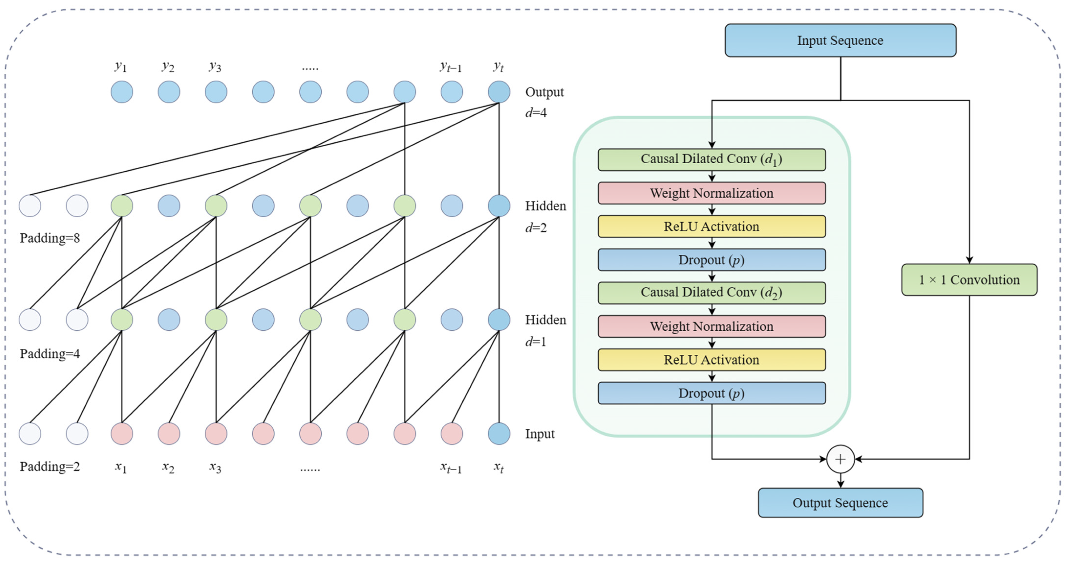
Here, F(x) is the residual mapping generated by convolutional transformation. For lithium-ion battery capacity data, TCN is effective at describing local temporal patterns during capacity fade and is especially suitable for representing regeneration behavior, short-term fluctuations, and near-neighbor degradation features [14,21,28]. The structure of the TCN module is shown in Figure 1.

2.4. Attention Mechanism (AM)

The attention mechanism (AM) automatically assigns different weights to different time steps or feature dimensions so that the model concentrates on the most informative content. Because battery degradation is not equally informative at every cycle, such reweighting helps the model respond more strongly to key stages and inflection behavior [28].
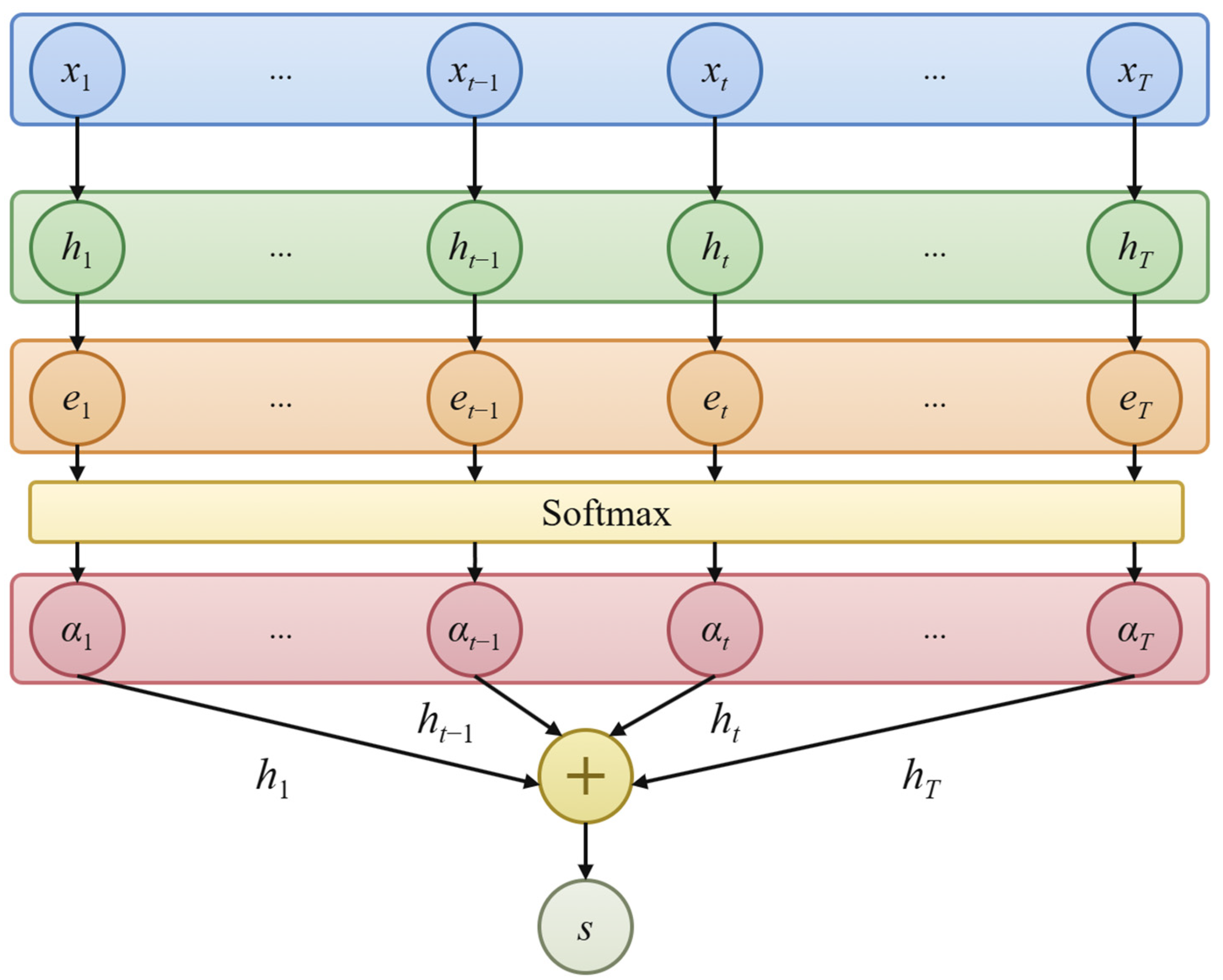
Let the hidden-state sequence output by TCN be {ht}t=1T. The attention scoring process can be expressed as
e t = u tan h ( W h t + b ) ,
where W and u are learnable parameters, and b is the bias term. The attention weights are then obtained through softmax normalization:
α t = e x p ( e t ) j = 1 T e x p ( e j ) .
The final weighted representation is
s = t = 1 T α t h t .
In essence, this mechanism reweights temporal features according to their importance. Time steps containing more salient degradation inflection points, abnormal fluctuations, or trend-transition information receive larger weights, thereby strengthening the representation of critical degradation evidence [28]. The AM structure is shown in Figure 2.

2.5. Transformer

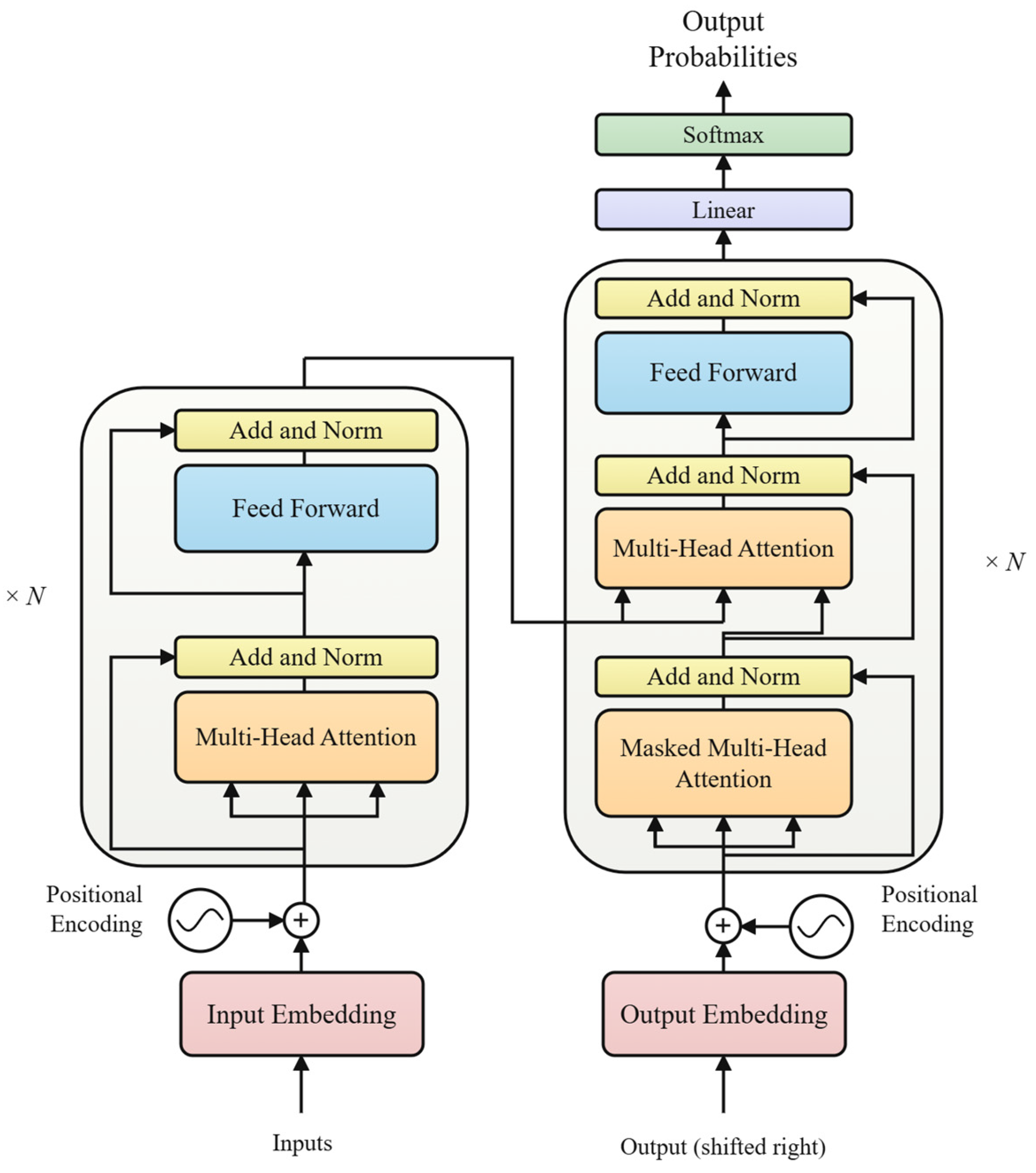
The Transformer is a self-attention-based deep sequence model that can directly establish dependencies between arbitrary temporal positions, making it particularly suitable for capturing long-range degradation correlations. In lithium-ion battery capacity prediction, the Transformer can effectively learn long-term degradation trends across cycles and compensate for the limited global modeling ability of purely local architectures [29].
Let the input sequence be represented by X. The Transformer first obtains the query, key, and value matrices through linear mapping:
Q = X W Q , K = X W K , V = X W V .
The global context representation is then computed through scaled dot-product attention:
A t t e n t i o n ( Q , K , V ) = s o f t m a x Q K T d k V ,
where dk is the key-vector dimension. To improve the ability of the model to extract information from different representation subspaces, the Transformer further adopts a multi-head mechanism:
M u l t i H e a d ( Q , K , V ) = C o n c a t ( head 1 , , head h ) W O .
After self-attention, the Transformer uses a feed-forward network to perform nonlinear mapping on the features:
F F N ( x ) = max ( 0 , x W 1 + b 1 ) W 2 + b 2 .
Together with residual connections and layer normalization, the Transformer can provide stronger global representation capability while maintaining stable training [29]. This makes it especially suitable for modeling long-term degradation trends in battery RUL prediction. The basic Transformer architecture is presented in Figure 3.

2.6. Overall Prediction Framework

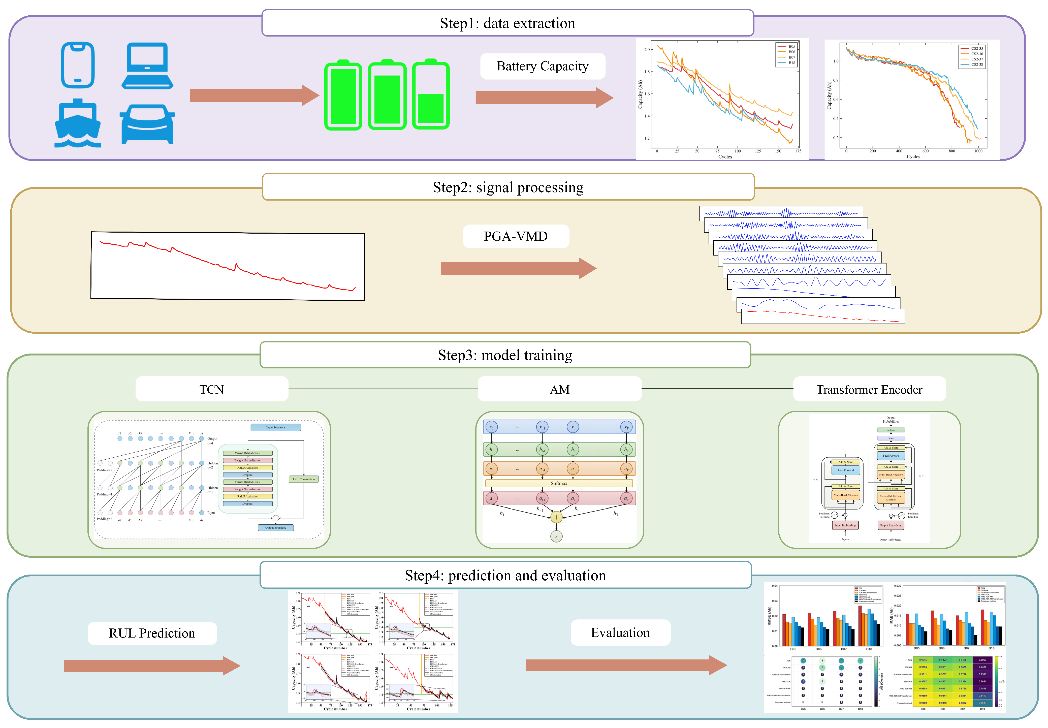
The proposed framework connects decomposition and prediction through three stages: adaptive decomposition of the raw capacity sequence, component-wise temporal forecasting, and reconstruction of the future capacity trajectory. PGA is first used to search for suitable VMD parameters so that the original sequence can be separated into components with clearer statistical roles. The regrouped components are then forecast by a deep temporal model, and their outputs are finally combined to recover the future capacity curve and the associated RUL. The overall workflow is illustrated in Figure 4.

2.6.1. Adaptive PGA-VMD Decomposition

Although conventional VMD can separate frequency components in battery capacity data, its effectiveness depends strongly on the choice of the mode number K and penalty factor α. Instead of determining these parameters empirically, this study employs PGA to identify them adaptively. Let the parameter vector be
z = [ α , K ] .
PGA searches for the optimal parameter combination z* within a predefined space so that the decomposed modes exhibit better separability and lower complexity. Here, the fitness function is constructed from the fuzzy entropy of the decomposed components and is expressed as
J ( α , K ) = m i n k F u z z y E n ( u k ) ,
where FuzzyEn(uk) represents the fuzzy entropy of the k-th component. A lower fuzzy entropy corresponds to a more regular and stable mode, which is generally easier for the subsequent predictor to learn. By minimizing this objective, PGA adaptively searches for K and α.
After optimization, the original capacity degradation sequence x(t) is decomposed using the optimal parameter set (α*, K*):
{ u k ( t ) } k = 1 K * = V M D ( x ( t ) ; α * , K * ) , x ( t ) = k = 1 K * u k ( t ) .
Compared with empirically configured VMD, PGA-guided decomposition adapts the decomposition scale to the statistical properties of the capacity sequence. This helps separate the slow attenuation trend from local fluctuations more clearly and reduces the influence of noise, regeneration, and other nonstationary disturbances on the subsequent prediction stage.
Compared with particle swarm optimization (PSO)-guided VMD [23] and sparrow search algorithm (SSA)-based tuning strategies in battery prognostics [19], PGA is used here, because its light-zone/shadow-zone evolution, mutation, and curvature-guided elongation provide a balanced exploration–exploitation process with a small number of control parameters [27]. This is suitable for the mixed discrete–continuous search of the VMD mode number K and penalty factor alpha. Moreover, the optimized VMD outputs are not fed directly to a single predictor; instead, they are regrouped into trend and fluctuation branches, which reduces the predictor burden and supports the subsequent hierarchical TCN-AM-Transformer design.

2.6.2. Component-Wise TCN-AM-Transformer Prediction

After PGA-VMD decomposition, the resulting subsequences are converted into supervised-learning samples using a sliding-window strategy, so that the model predicts the next capacity value from historical observations. For an input sample X, the local temporal features extracted by the TCN are
H = TCN ( X ) .
At this stage, the TCN focuses on local degradation patterns and short-term fluctuations, which is particularly useful for describing fine-scale changes induced by varying charge-discharge conditions, local capacity recovery, and measurement disturbances.
An AM module is then inserted after the TCN to emphasize informative time steps. Following the formulation in [28], the hidden states are used to compute attention scores and normalized weights. To preserve the full temporal structure for the downstream Transformer encoder, these weights are applied as gating coefficients to the features at each time step, yielding a reweighted sequence:
h ~ t = α t h t , H ~ = [ h ~ 1 , h ~ 2 , , h ~ T ] .
After reweighting, informative degradation stages are amplified, whereas redundant or weakly relevant information is suppressed, which facilitates the subsequent global modeling process.
The attention-weighted sequence H is then sent to the Transformer encoder to model long-range dependence across time as
Z = T r a n s f o r m e r E n c o d e r ( H ~ ) .
The encoder output is subsequently passed through a fully connected layer and a regression mapping to obtain the one-step-ahead capacity prediction:
y ^ t + 1 = f reg ( F C ( Z ) ) .
In this way, the TCN-AM-Transformer predictor integrates local pattern extraction, feature reweighting, and global dependency learning. TCN captures multi-scale local degradation information, AM highlights key temporal evidence, and the Transformer models long-horizon evolution; thus, the three modules complement one another [28,29].

2.6.3. Capacity Reconstruction and RUL Inference

Within the complete framework, PGA-VMD is used for the adaptive decomposition of the original capacity sequence, whereas TCN-AM-Transformer performs temporal prediction on the regrouped subsequences. Their combination improves RUL estimation from both signal-processing and sequence-modeling perspectives.
Modeling each decomposed mode individually significantly increases the network complexity. Since several high-frequency components exhibit statistically similar fluctuation properties, this paper regroups the VMD results prior to deep feature extraction. The low-frequency component that reflects the dominant degradation trend is denoted by x L ( t ) , and the high-frequency components that characterize local fluctuations and disturbances are aggregated as x H ( t ) , namely,
x L ( t ) = k Ω L u k ( t ) , x H ( t ) = k Ω H u k ( t ) ,
where Ω L and Ω H denote the low-frequency and high-frequency mode sets, respectively. Then, x L ( t ) and x H ( t ) are fed into two isomorphic TCN-AM-Transformer subpredictors to obtain the corresponding predictions. The final total capacity prediction is reconstructed in the time domain as
x ^ ( t + 1 ) = x ^ L ( t + 1 ) + x ^ H ( t + 1 ) .
From this perspective, the method can be viewed as a hierarchical prediction strategy. PGA-VMD first transforms the original strongly coupled capacity sequence into simpler subsequences, thereby reducing nonstationarity and easing the modeling task. The deep predictor then learns the dominant degradation trend and local fluctuation information separately before recombining them to recover the complete capacity-evolution trajectory. Compared with direct prediction on the raw sequence, this design is better suited to representing degradation information at different scales.
RUL is inferred from the reconstructed capacity curve by locating the first cycle at which the predicted capacity crosses the failure threshold. The difference between that cycle and the current cycle is taken as the predicted RUL. In this manner, the proposed framework forms a complete pipeline from adaptive decomposition to component prediction, trajectory reconstruction, and lifetime estimation. Its main strengths are that PGA reduces subjectivity in VMD parameter selection, VMD improves degradation-sequence separability, and the TCN-AM-Transformer network jointly models local features, salient information, and long-range dependence, which is well matched to the complex degradation behavior of lithium-ion batteries [14,21,28].

3. Experimental Design

3.1. Description of Lithium-Ion Battery Datasets

The proposed approach is validated using the public NASA, CALCE, and BIT battery datasets.
NASA: Four 18650 lithium-ion batteries, B05, B06, B07, and B18, cycled at room temperature (about 24 °C), are selected from the NASA dataset. Each cell has a rated capacity of 2 Ah. Charging follows a constant-current/constant-voltage (CC-CV) protocol: the cells are charged at 1.5 A until 4.2 V and then held at constant voltage until the current decreases to 20 mA. During discharge, the cells are discharged at 2 A to a cutoff voltage between 2.2 V and 2.7 V. The dataset includes charge–discharge records together with electrochemical impedance spectroscopy (EIS) measurements.
CALCE: Four LiCoO2-based batteries, CS2_35, CS2_36, CS2_37, and CS2_38, tested at room temperature, are selected from the CALCE dataset. Their rated capacity is about 1.1 Ah. Charging also follows a CC-CV protocol: the cells are charged at 0.5 C to 4.2 V and then maintained at constant voltage until the current falls to 0.05 A. Discharge is performed under a 1 C constant-current regime with a cutoff voltage of 2.7 V.
BIT: Three Panasonic NCR18650BD cylindrical cells, BIT-01, BIT-02, and BIT-03, from the BIT dataset reported by Lu et al. [30], are used as supplementary higher-capacity cells. They have a nominal capacity of 3.03 Ah, are cycled under multiple charge–discharge protocols at 20 °C, and use an EOL threshold of 2.424 Ah (80% of nominal capacity).
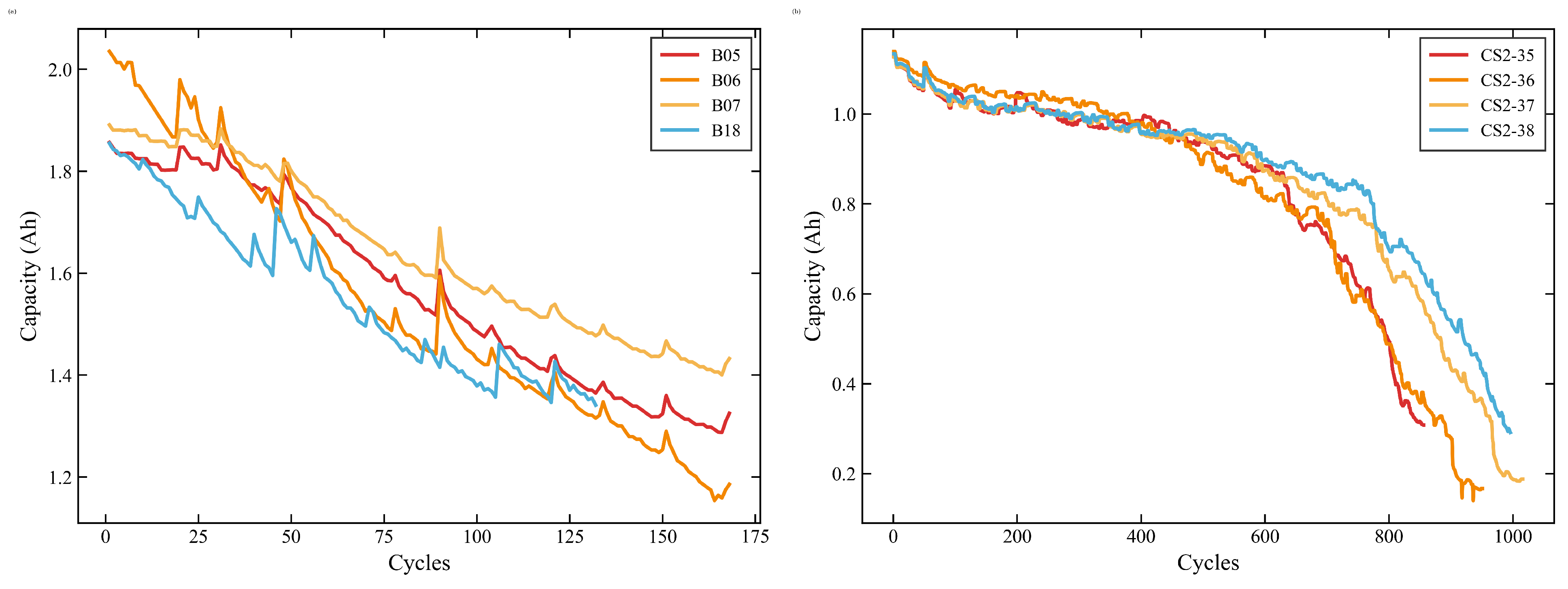
For subsequent modeling and evaluation, the discharge capacity indexed by cycle is used as the main health indicator. The EOL threshold is set to 1.40 Ah for the NASA cells except B07, for which 1.44 Ah is used; for CALCE-CS2, the threshold is 0.88 Ah; for BIT cells, the threshold is 2.424 Ah. The NASA and CALCE capacity-degradation trajectories are presented in Figure 5; the BIT trajectories and metrics are reported in Section 4.1.3.

3.2. Data Preprocessing

Because the decomposed trend and fluctuation components can differ substantially in scale, min–max normalization is applied to the available training/historical data and the corresponding prediction inputs so that the inputs lie within [0, 1]. This reduces the bias caused by scale differences and facilitates network convergence. The normalization formula is [17]
x ( t ) = x ( t ) x m i n x m a x x m i n ,
where x(t) denotes the original sequence, x′(t) denotes the normalized sequence, and xmin and xmax are the minimum and maximum values fitted from the historical/training portion available before prediction. Specifically, for each prediction case, the scaler is fitted only with observations not later than the starting point (SP), and the same fixed parameters are then used to normalize the subsequent prediction interval. No future capacity values after the SP are used to calculate normalization parameters. After prediction, inverse normalization is applied using the same fixed parameters so that the results can be evaluated on the original physical scale:
x p ( t ) = x p ( t ) ( x m a x x m i n ) + x m i n ,
where x p (t) denotes the normalized model output, and xp(t) is the final prediction restored to the true capacity scale. This preprocessing step provides consistent inputs for subsequent feature learning while maintaining a leakage-free evaluation protocol.

3.3. Definition of Remaining Useful Life (RUL)

Capacity fade is the most direct observable manifestation of irreversible aging during repeated cycling of lithium-ion batteries. Once the capacity falls to a preset EOL threshold, the battery is considered to have reached the end of its service life. In engineering practice and the related literature, this threshold is often set to 70–80% of the rated capacity to balance usability and safety.
For cycle-level lifetime prediction, the RUL is defined as the number of remaining charge–discharge cycles from the starting point (SP) to the EOL threshold. Let ti denote the current cycle index at the prediction instant, and let tEOL denote the cycle index corresponding to EOL. Following [28], the RUL is calculated as
RUL i = t E O L t i .
In practical evaluation, the capacity trajectory is predicted first, after which the intersection between the predicted curve and the EOL threshold is used to locate tEOL and determine the corresponding RUL. This trajectory-to-threshold strategy is widely adopted in studies that jointly predict the capacity and lifetime.

3.4. Evaluation Metrics

This study uses four quantitative metrics: RMSE, MAE, R2, and AE. RMSE and MAE measure the magnitude of prediction error, R2 evaluates the agreement between predicted and true trajectories, and AE quantifies the absolute deviation of RUL prediction on the cycle scale.
Assume that there are N sample points in the evaluation interval, the true-value sequence is denoted by y k (k = 1, …, N), with mean y , and the predicted-value sequence is denoted by y ^ k (k = 1, …, N), where y can denote capacity, RUL, or another target quantity. The metrics are defined as follows:
(1) MAE [31]
MAE = 1 N k = 1 N y k y ^ k ,
(2) RMSE [32]
RMSE = 1 N k = 1 N y k y ^ k 2 ,
(3) R2 [31]
R 2 = 1 k = 1 N y k y ^ k 2 k = 1 N y k y 2 ,
(4) AE for RUL evaluation [33]
Let RULt and RULp denote the true and predicted RUL values, respectively, in cycles. Then,
AE = R U L t R U L p ,
Lower values of MAE, RMSE, and AE indicate better performance, whereas an R2 value closer to 1 indicates stronger fitting consistency.

3.5. Experimental Setup

All experiments were carried out on a Windows 11 (64-bit) workstation equipped with an Intel Core i9-14900HX CPU, 32 GB RAM, and an NVIDIA GeForce RTX 4060 Laptop GPU with 8 GB of video memory. The deep-learning models were implemented in Python 3.8 using PyCharm 2025.2.0.1, and model construction and training were completed with TensorFlow 2.6.1 and Keras 2.6.0.
Within-cell experiments were split chronologically: cycles 1 to SP formed the training/historical subset, and post-SP cycles were reserved for testing, with no sliding-window sample crossing the SP boundary. After PGA-VMD decomposition and regrouping, the low-frequency and aggregated high-frequency components were separately converted into supervised samples using a window length of 10 and a stride of 1, producing SP-10 training samples and N-SP-10 test samples for a sequence of length N. Each cell was modeled independently. Adam was used with a learning rate of 1 × 10⁻⁴, batch size of 5, and 100 epochs; The PGA search ranges were K from 8 to 12 and α from 800 to 2000 for NASA, and α from 1000 to 2500 for CALCE and BIT. Post-SP trajectories were obtained by rolling one-step-ahead prediction, and the first EOL-threshold crossing determined the predicted RUL. For the in-house baseline comparisons, all variants used the same SP for each cell.
The implemented predictor contains 119,507 trainable parameters, requires approximately 2.57 MFLOPs (2,565,421 FLOPs) for one input sample, and takes 0.3577 ms per sample on the workstation. This suggests a light online burden for cycle-level RUL inference: PGA-VMD search and model updates can be scheduled offline or periodically, while the BMS online operation uses fixed decomposition settings and the trained predictor.

4. Results

4.1. Comparison with Baseline Models

To evaluate both the prediction accuracy and generalization of the proposed PGA-VMD-TCN-AM-Transformer, comparative experiments are conducted on the NASA and CALCE datasets against six baseline models: TCN, TCN-AM, TCN-AM-Transformer, VMD-TCN, VMD-TCN-AM, and VMD-TCN-AM-Transformer. Additional experiments are conducted on the BIT dataset to examine the performance under a higher-capacity degradation scenario. The RMSE, MAE, AE, and R2 are used to characterize the full-trajectory fitting error, average deviation, end-point error in RUL, and consistency with the observed degradation path.

4.1.1. NASA Dataset

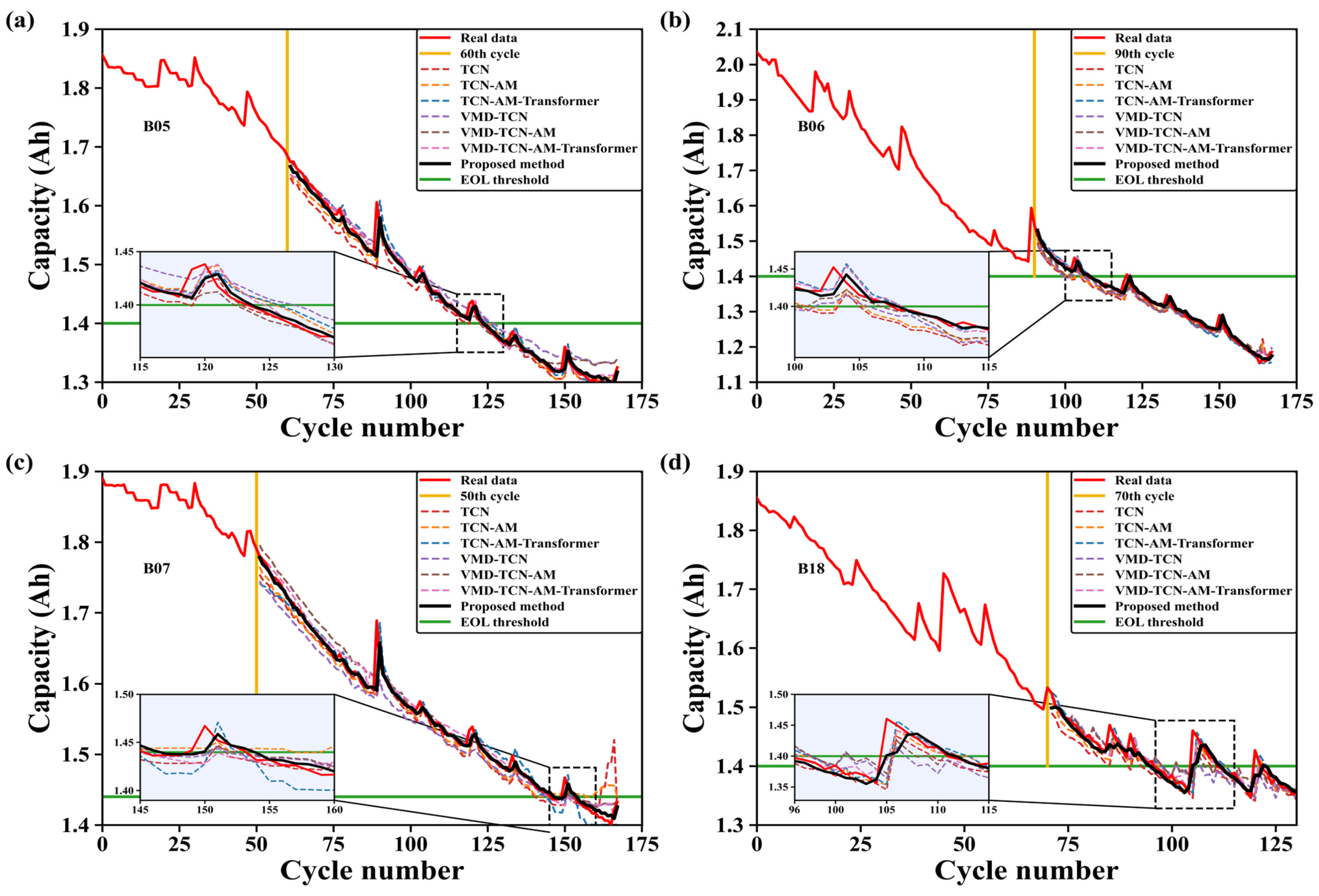
The NASA dataset is used to evaluate the method under short-life conditions with pronounced local fluctuations. As shown in Figure 6, the proposed model follows the dominant capacity-decay trend closely after the prediction starting point while still tracking local rebounds and irregular disturbances. In the enlarged EOL views, the predicted and measured curves intersect the threshold at nearly the same cycle, without obvious early or late crossing. This behavior indicates that the model retains both global trend awareness and end-point sensitivity.
Comparison across variants provides further insight. A standalone TCN accumulates noticeable deviation on strongly nonstationary cells such as B06 and B18, indicating that direct modeling of the raw sequence is insufficient. Adding AM brings the predicted curves closer to the measured trajectories for most cells, which implies better emphasis on informative degradation stages. When the Transformer is included, the long-range trend consistency improves further. Once VMD is introduced, the predictions become less sensitive to local regeneration and noise, confirming the value of modal decomposition. With PGA-based parameter tuning, the proposed method yields the most stable threshold localization and the most consistent trajectory fit across the four NASA cells.
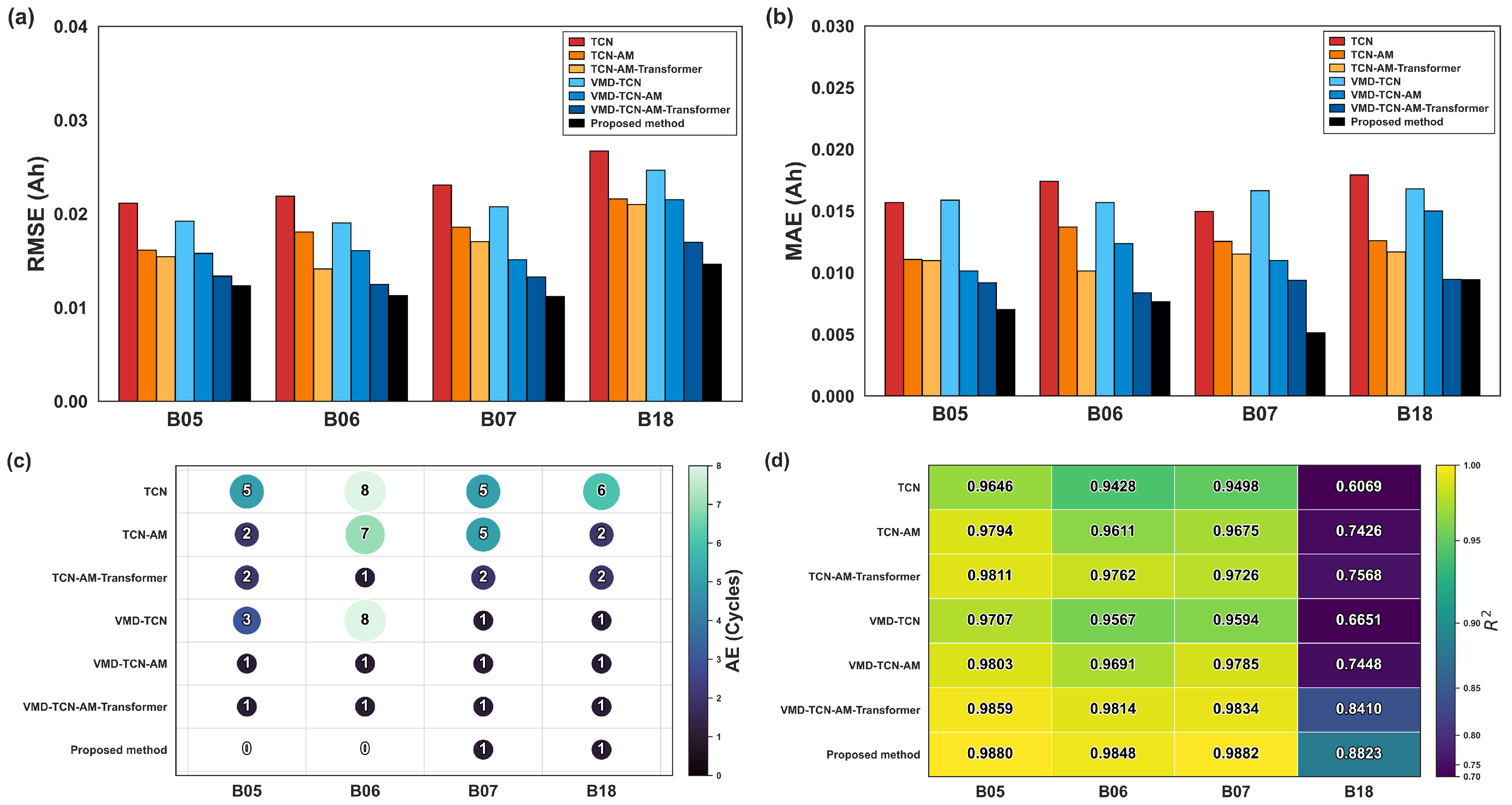
The quantitative evidence shown in Figure 7 agrees with these visual observations. Across the four NASA batteries, the proposed method achieves the best or jointly best results for all metrics. The RMSE remains below 0.015 Ah for every cell, the MAE stays below 0.010 Ah, and the AE is confined to 0–1 cycle. On average, the RMSE and MAE drop to 0.0123 Ah and 0.0073 Ah, representing improvements of 11.9% and 19.7% over the strongest baseline, VMD-TCN-AM-Transformer. The mean AE also decreases from 1.0 cycle to 0.5 cycle. The EOL error is zero for B05 and B06, and even the more irregular B07 and B18 are predicted within 1 cycle.
Overall, the NASA experiments indicate that AM and the Transformer enhance the temporal feature extraction, VMD reduces the error accumulation caused by nonstationary fluctuations, and PGA further stabilizes the decomposition and end-point localization. The combined framework therefore delivers more reliable RUL estimation under short-life degradation conditions. Detailed numerical results are listed in Table 1.

4.1.2. CALCE Dataset

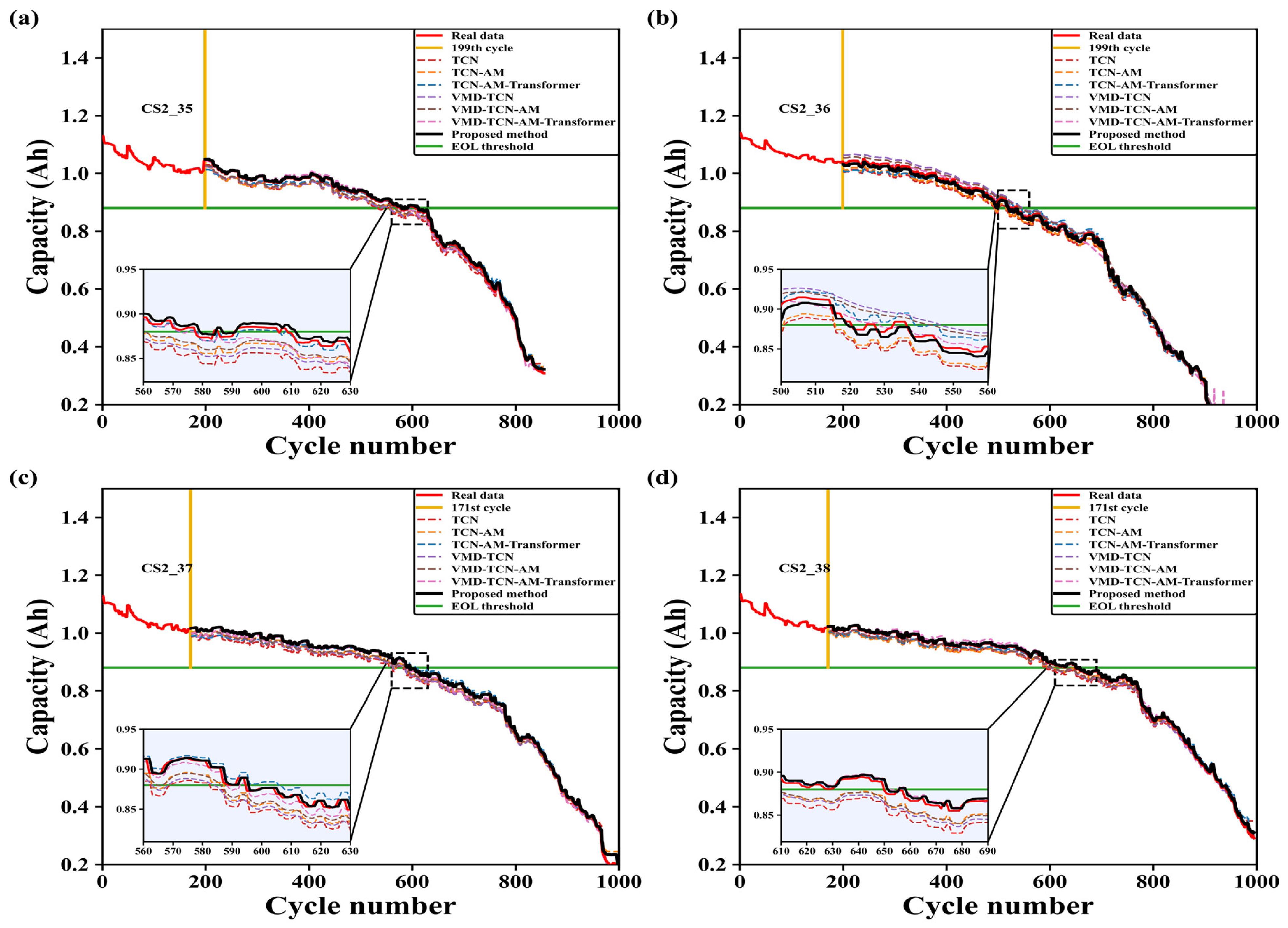
Compared with NASA, the CALCE dataset provides longer degradation trajectories and a substantially longer extrapolation interval, making it a more demanding test of model generalization. As illustrated in Figure 8, the proposed model reconstructs the multi-stage degradation behavior, including slow decay, plateau-like intervals, and rapid decline, with high fidelity. The predicted curves remain close to the measurements on all four cells, and the magnified EOL regions show accurate capture of both the slope change and threshold crossing.
The baseline results again show the benefit of decomposition. TCN-based models without VMD are more susceptible to cumulative drift during long-horizon extrapolation, which can produce early or late failure-time judgments. Adding AM and the Transformer improves global trend modeling, but some late-stage inflection behavior is still not handled stably. After VMD is introduced, the trajectories become smoother, and local errors are reduced for most cells. PGA-based tuning further improves the fit near the EOL and avoids excessive smoothing around the failure point, indicating that adaptive decomposition is beneficial for subsequent temporal learning.
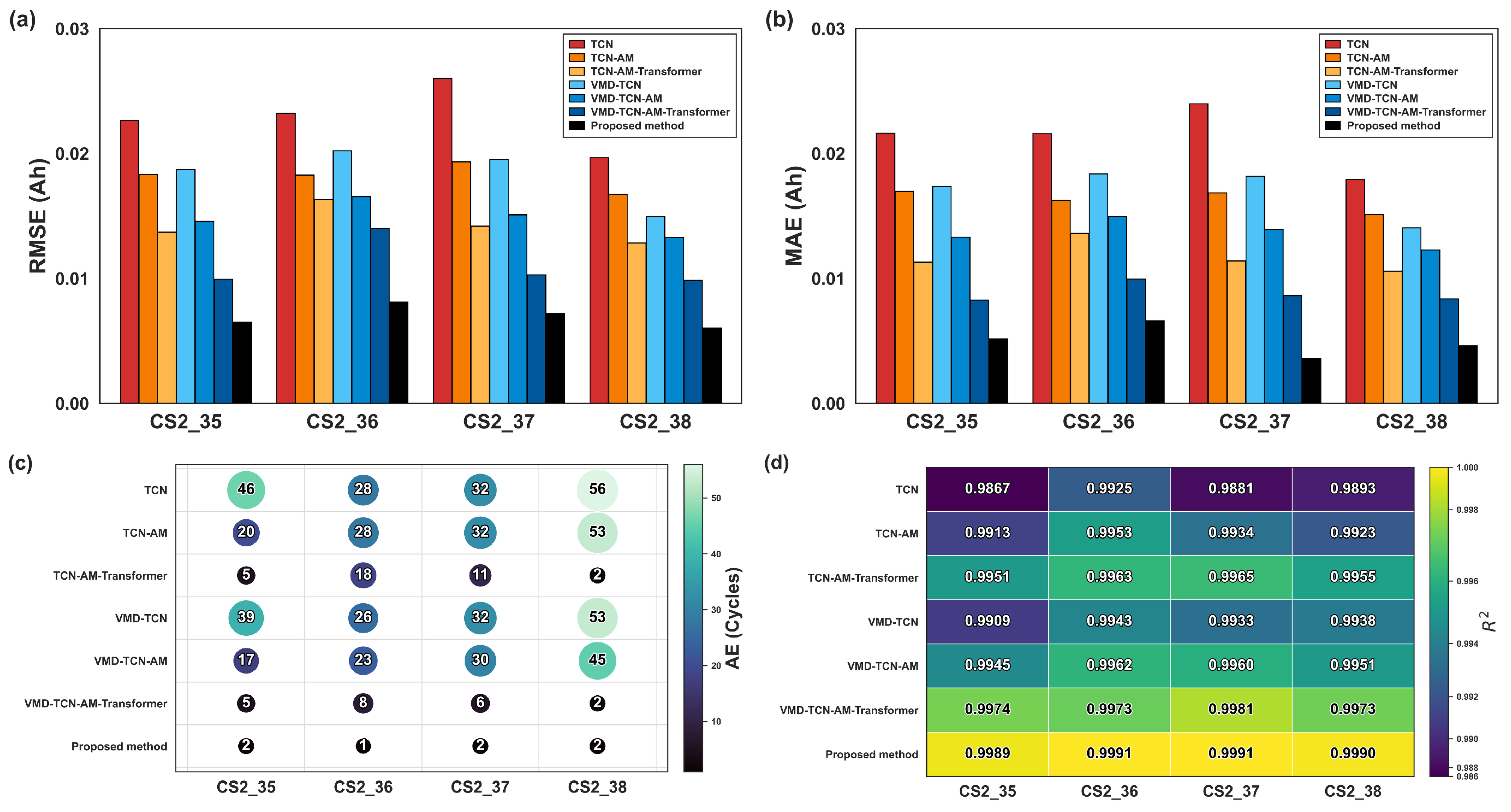
As summarized in Figure 9, the proposed approach again achieves the best or jointly best performance among the evaluated baselines. The average RMSE and MAE are 0.00695 Ah and 0.00499 Ah, respectively, which are 36.9% and 43.2% lower than those of VMD-TCN-AM-Transformer. All four cells yield R2 values above 0.9989, and the AE remains within 1–2 cycles, with a mean of 1.75 cycles. By comparison, the best baseline still has an average AE of 5.25 cycles. These results indicate that the proposed method not only fits the trajectory accurately but also reduces the end-point deviation in long-life prediction.
A closer look at individual cells highlights the same pattern. For CS2_35 and CS2_36, conventional TCN-based variants exhibit large threshold-localization errors, whereas the proposed method reduces the AE to 2 and 1 cycles, respectively. For CS2_37, the MAE falls to 0.00359 Ah, revealing strong fine-grained fitting capability. For CS2_38, whose late-stage degradation is smoother but still locally intricate, the proposed model achieves the lowest RMSE and the highest R2, demonstrating good adaptability to gradual long-life decay.
These results show that the PGA-VMD-TCN-AM-Transformer is effective not only for short-life batteries with stronger fluctuations but also for long-life cells that require stable long-range extrapolation. The method therefore exhibits solid cross-scenario applicability and practical promise. Table 2 reports the full numerical comparison.

4.1.3. BIT Dataset

The BIT dataset used in this study, reported by Lu et al. [30], contains Panasonic NCR18650BD cylindrical lithium-ion cells with a nominal capacity of 3.03 Ah cycled under multiple charge–discharge protocols at 20 °C. Charging follows a 0.3 C constant-current/constant-voltage procedure to 4.2 V with a cutoff current of 0.03 A, and discharge is performed at 2 C to the manufacturer-specified cutoff voltage; all tests were recorded with an ARBIN BT2000 battery cycler. Following the dataset definition, the EOL threshold is set to 2.424 Ah (80% of nominal capacity) [30].
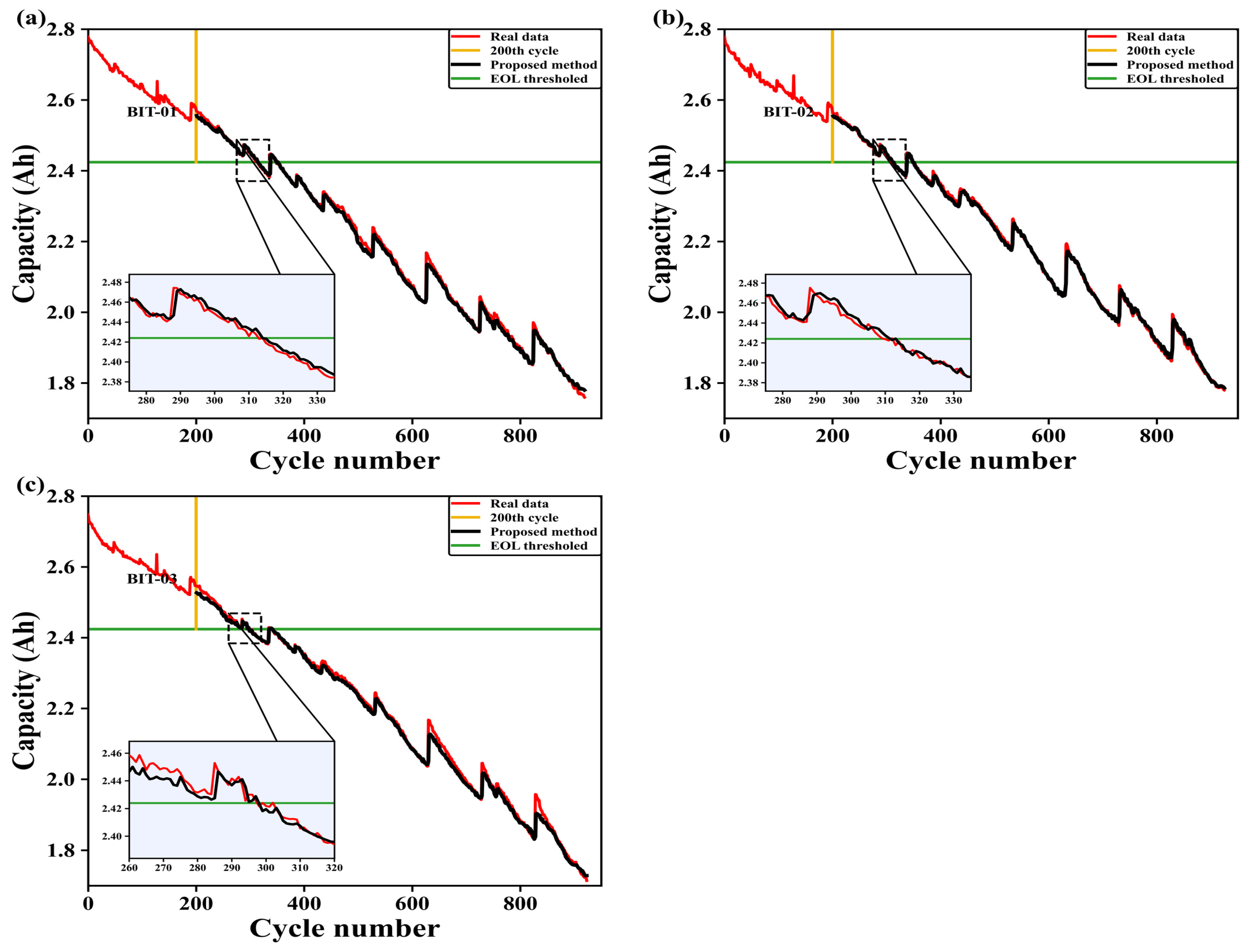
To examine whether the proposed framework remains stable for higher-capacity cells, three BIT cells, denoted BIT-01, BIT-02, and BIT-03, are evaluated with the same prediction starting point, SP = 200. The predicted trajectories are shown in Figure 10, and the numerical metrics are summarized in Table 3.
As shown in Figure 10, the proposed method reconstructs the main degradation path after the 200th cycle while following recurrent local recovery segments. The enlarged EOL regions show that the predicted threshold intersections are close to the measured intersections for all three cells, suggesting that PGA-VMD effectively separates the global capacity fade from local oscillations and helps the downstream TCN-AM-Transformer predictor retain EOL sensitivity.
Quantitatively, the RMSE ranges from 0.01007 Ah to 0.01358 Ah, and the MAE remains below 0.00928 Ah for all BIT cells. The R2 values are higher than 0.9963, and the AE is no more than 2 cycles. The average RMSE, MAE, and AE are 0.01201 Ah, 0.00771 Ah, and 1.0 cycle, respectively. These results verify that the proposed method maintains accurate capacity tracking and threshold localization when applied to the BIT cells.
Taken together, the NASA, CALCE, and supplementary BIT results show that AM and the Transformer improve the temporal representation, VMD increases the resilience to regeneration-related fluctuations, and PGA-based tuning further improves the decomposition quality, component reconstruction, and threshold localization under the 2.424 Ah BIT EOL setting.

4.2. Comparison with Other Methods

To place the proposed framework in the context of recent literature, its performance is compared with representative hybrid and decomposition-based methods reported in published studies. Different studies, however, may adopt different prediction starting points (SPs), train–test splits, and evaluation protocols. Therefore, unlike the in-house comparisons in Table 1 and Table 2, where all baseline variants are evaluated under identical SPs for each cell, the literature comparisons in Table 4 and Table 5 retain the SPs reported in the original papers and should be interpreted as reference-level comparisons rather than strict head-to-head rankings.
For the NASA dataset in Table 4, the rows with the same or nearly the same SP provide the most informative comparison. On B05, the proposed method uses SP = 60, which is identical to TCN-GRU-DNN with dual attention [14] and close to CNN-LSTM-DNN [13] with SP = 61; it achieves a lower RMSE than both, although the MAE is slightly higher than that of [14]. On B07 and B18, the proposed method is compared at the same or adjacent SPs as several published models and remains competitive in both RMSE and MAE. For B06, the proposed SP = 90 is later than most reported literature SPs; so, the shorter extrapolation horizon may benefit the numerical errors; this result is therefore used only as supplementary evidence of stable tracking under the selected benchmark setting, not as a direct superiority claim over all published methods.
For the CALCE dataset in Table 5, the same caution applies. On CS2_35 and CS2_36, the proposed method is evaluated at SP = 199, matching the setting of TCN-GRU-DNN with dual attention [14] and, for CS2_36, CNN-LSTM-DNN [13]. On CS2_37 and CS2_38, several methods use the same SP = 171, making these rows more comparable; the proposed method achieves the smallest MAE on CS2_37 and the lowest RMSE and MAE on CS2_38. The results from methods using substantially later SPs, such as SP = 241, 271, or 283, are retained for completeness but should be interpreted cautiously, because later SPs generally shorten the prediction horizon and may reduce the difficulty of RUL estimation.
In short, the literature tables indicate that the proposed framework is competitive within the range of reported benchmark settings, especially when same-SP or near-SP rows are considered. The main evidence for fair model-to-model comparison remains the controlled baseline experiments in Table 1 and Table 2, while Table 4 and Table 5 serve as reference-level comparisons for positioning the method relative to recent studies.

4.3. Discussion

The experimental evidence from NASA, CALCE, and the supplementary BIT validation suggests that the proposed framework improves the prediction quality through the coordinated action of adaptive decomposition and hierarchical sequence modeling. PGA-optimized VMD reduces the difficulty of learning directly from raw nonstationary capacity signals, while TCN, AM, and the Transformer contribute complementary abilities: local pattern extraction, emphasis on informative degradation stages, and modeling of long-range temporal dependence. The steady gains observed across progressive baseline variants indicate that the improvement does not originate from any single module in isolation but from their interaction within the full framework. This emphasis on combining short-range and long-range sequence learning is also consistent with recent battery SOH estimation work that integrates LSTM and iTransformer architectures with data augmentation [36].
From a structural viewpoint, the framework is not a direct concatenation of VMD, TCN, AM, and Transformer modules. PGA first adapts the VMD scale to the current capacity trajectory; the decomposed modes are then regrouped into trend-dominant and fluctuation-dominant branches; AM acts as a gating stage between local TCN extraction and global Transformer encoding; and the final RUL estimate is obtained after branch-wise reconstruction of the physical capacity curve. This decomposition–regrouping–gating–reconstruction path distinguishes the method from one-stage VMD-based hybrid pipelines and explains why the gains remain consistent across datasets [21,22,23,24].
Several limitations should nevertheless be acknowledged. Although the additional BIT experiment indicates that the decomposition and temporal modeling strategy can retain useful degradation representations under a higher-capacity dataset, the present validation is still based on public laboratory datasets and cycle-based discharge capacity. Its transferability to newer battery chemistries, larger field datasets, and more dynamic charging/discharging profiles remains to be verified. Future work should therefore examine operation-rich datasets, update or streaming strategies, and the latency, memory, and computational constraints imposed by strict online BMS deployment.

5. Conclusions

To address the challenges posed by regeneration, local fluctuations, and long-horizon dependencies in lithium-ion battery degradation, this paper proposes a PGA-VMD-TCN-AM-Transformer framework for RUL prediction. PGA adaptively determines the VMD parameters, the capacity sequence is decomposed and regrouped into trend and fluctuation branches, and a hierarchical TCN-AM-Transformer predictor performs component-wise forecasting before reconstructing the final capacity trajectory and RUL.
Comparative analyses indicate that PGA enhances the decomposition adaptivity, VMD reduces the influence of regeneration and local noise, and the hierarchical TCN-AM-Transformer architecture strengthens the representation of both local and long-range degradation information. The performance gain therefore comes from adaptive decomposition-regrouping and branch-wise prediction–reconstruction rather than from simple module stacking. These results demonstrate that the proposed framework is accurate, robust, and promising for lithium-ion battery RUL prediction.

Author Contributions

Conceptualization, S.W. and Z.N.; Methodology, S.W.; Software, S.W. and L.Z.; Validation, S.W. and L.Z.; Formal Analysis, S.W.; Investigation, S.W. and L.Z.; Resources, Z.N. and L.L.; Data Curation, S.W. and L.Z.; Writing—Original Draft Preparation, S.W. and L.Z.; Writing—Review and Editing, Z.N. and L.L.; Supervision, Z.N. All authors have read and agreed to the published version of the manuscript.

Funding

This work was supported by the Start-up Foundation of Nanjing University of Information Science and Technology.

Institutional Review Board Statement

Not applicable.

Informed Consent Statement

Not applicable.

Data Availability Statement

Publicly available datasets were analyzed in this study. The NASA Li-ion Battery Aging Datasets are available from the NASA Open Data Portal, the CALCE battery datasets are available from the CALCE Battery Research Data repository, and the BIT dataset used in this study is described by Lu et al. [30].

Conflicts of Interest

The authors declare no conflicts of interest.

References

  1. Madani, S.S.; Shabeer, Y.; Allard, F.; Fowler, M.; Ziebert, C.; Wang, Z.; Panchal, S.; Chaoui, H.; Mekhilef, S.; Dou, S.X.; et al. A comprehensive review on lithium-ion battery lifetime prediction and aging mechanism analysis. Batteries 2025, 11, 127. [Google Scholar] [CrossRef]
  2. Wu, L.; Fu, X.; Guan, Y. Review of the remaining useful life prognostics of vehicle lithium-ion batteries using data-driven methodologies. Appl. Sci. 2016, 6, 166. [Google Scholar] [CrossRef]
  3. Fu, L.; Jiang, B.; Zhu, J.; Wei, X.; Dai, H. Early remaining useful life prediction for lithium-ion batteries using a Gaussian process regression model based on degradation pattern recognition. Batteries 2025, 11, 221. [Google Scholar] [CrossRef]
  4. Wang, S.; Ma, H.; Zhang, Y.; Li, S.; He, W. Remaining useful life prediction method of lithium-ion batteries is based on variational modal decomposition and deep learning integrated approach. Energy 2023, 282, 128984. [Google Scholar] [CrossRef]
  5. Zhao, F.; Dai, X. A hybrid RUL prediction approach for lithium-ion batteries based on CEEMDAN-SSA-SVR-BiGRU. ICCK Trans. Syst. Saf. Reliab. 2025, 1, 136–148. [Google Scholar] [CrossRef]
  6. Wang, Z.; Liu, Y.; Wang, F.; Wang, H.; Su, M. Capacity and remaining useful life prediction for lithium-ion batteries based on sequence decomposition and a deep-learning network. J. Energy Storage 2023, 72, 108085. [Google Scholar] [CrossRef]
  7. Wang, X.; Ye, P.; Liu, S.; Zhu, Y.; Deng, Y.; Yuan, Y.; Ni, H. Research progress of battery life prediction methods based on physical model. Energies 2023, 16, 3858. [Google Scholar] [CrossRef]
  8. Xi, R.; Mu, Z.; Ma, Z.; Jin, W.; Ma, H.; Liu, K.; Li, J.; Yu, M.; Jin, D.; Cheng, F. Lifetime prediction of rechargeable lithium-ion battery using multi-physics and multiscale model. J. Power Sources 2024, 608, 234622. [Google Scholar] [CrossRef]
  9. Chen, L.; Ding, S.; Wang, L.; Zhu, F.; Zhu, X.; Zhang, S.; Dai, H.; He, X.; Cao, G.; Qiu, J.; et al. Electrochemical model boosting accurate prediction of calendar life for commercial LiFePO4/graphite cells by combining solid electrolyte interface side reactions. Appl. Energy 2024, 376, 124175. [Google Scholar] [CrossRef]
  10. Chen, D.; Zheng, X.; Chen, C.; Zhao, W. Remaining useful life prediction of the lithium-ion battery based on CNN-LSTM fusion model and grey relational analysis. Electron. Res. Arch. 2023, 31, 633–655. [Google Scholar] [CrossRef]
  11. Shi, Z.; Ibrahim, A.W.; Xu, J.; Zeng, L.; Farh, H.M.H.; Al-Shamma’a, A.A.; Ameur, K. Enhanced remaining useful life prediction of lithium-ion battery based on a dual attention hybrid data-driven method. Sci. Rep. 2026, 16, 1303. [Google Scholar] [CrossRef] [PubMed]
  12. Hu, J.; Fu, P.; Wei, Z.; Huang, Y.; Early, J.; Fly, A.; Zhang, Y. Early prediction of lithium-ion battery degradation with a generative pre-trained transformer. Nat. Commun. 2025, 17, 126. [Google Scholar] [CrossRef]
  13. Zraibi, B.; Okar, C.; Chaoui, H.; Mansouri, M. Remaining useful life assessment for lithium-ion batteries using CNN-LSTM-DNN hybrid method. IEEE Trans. Veh. Technol. 2021, 70, 4252–4261. [Google Scholar] [CrossRef]
  14. Li, L.; Li, Y.; Mao, R.; Li, L.; Hua, W.; Zhang, J. Remaining useful life prediction for lithium-ion batteries with a hybrid model based on TCN-GRU-DNN and dual attention mechanism. IEEE Trans. Transp. Electrif. 2023, 9, 4726–4740. [Google Scholar] [CrossRef]
  15. Zhao, S.; Sun, D.; Liu, Y.; Liang, Y. Remaining useful life prediction for lithium-ion batteries based on hybrid ensembles allied with data-driven approach. Energies 2025, 18, 1114. [Google Scholar] [CrossRef]
  16. Liu, K.; Shang, Y.; Ouyang, Q.; Widanage, W.D. A data-driven approach with uncertainty quantification for predicting future capacities and remaining useful life of lithium-ion battery. IEEE Trans. Ind. Electron. 2021, 68, 3170–3180. [Google Scholar] [CrossRef]
  17. Wang, J.; Zhang, S.; Li, C.; Wu, L.; Wang, Y. A data-driven method with mode decomposition mechanism for remaining useful life prediction of lithium-ion batteries. IEEE Trans. Power Electron. 2022, 37, 13684–13695. [Google Scholar] [CrossRef]
  18. Tang, T.; Yuan, H. A hybrid approach based on decomposition algorithm and neural network for remaining useful life prediction of lithium-ion battery. Reliab. Eng. Syst. Saf. 2022, 217, 108082. [Google Scholar] [CrossRef]
  19. Qiu, S.; Zhang, B.; Lv, Y.; Zhang, J.; Zhang, C. A lithium-ion battery remaining useful life prediction model based on CEEMDAN data preprocessing and HSSA-LSTM-TCN. World Electr. Veh. J. 2024, 15, 177. [Google Scholar] [CrossRef]
  20. Zhou, Y.; Li, Z.; Zhao, M.; Wu, F.; Yang, T. A transformer-based hybrid method with multi-feature for lithium battery remaining useful life prediction. J. Power Sources 2025, 655, 237844. [Google Scholar] [CrossRef]
  21. Wang, G.; Sun, L.; Wang, A.; Jiao, J.; Xie, J. Lithium battery remaining useful life prediction using VMD fusion with attention mechanism and TCN. J. Energy Storage 2024, 93, 112330. [Google Scholar] [CrossRef]
  22. Zou, B.; Li, R.; Ling, L. Remaining life prediction of lithium-ion batteries based on VMD decomposition and cascaded BiLSTM-Transformer network. J. King Saud Univ. Comput. Inf. Sci. 2026, 38, 55. [Google Scholar] [CrossRef]
  23. Zhang, L.; Du, X.; Diallo, D.; Delpha, C.; Benbouzid, M. Optimized VMD-Transformer framework for accurate remaining useful life prediction of lithium-ion batteries. IEEE Trans. Transp. Electrif. 2026, 12, 192–207. [Google Scholar] [CrossRef]
  24. Li, Y.; Li, L.; Li, L.; Huang, X.; Sun, G.; Wang, Y.; Zhang, J. Research on hybrid data-driven method for predicting the remaining useful life of lithium-ion batteries. Comput. Phys. Commun. 2025, 309, 109500. [Google Scholar] [CrossRef]
  25. Ding, G.; Wang, W.; Zhu, T. Remaining useful life prediction for lithium-ion batteries based on CS-VMD and GRU. IEEE Access 2022, 10, 89402–89413. [Google Scholar] [CrossRef]
  26. Xu, W.; Li, Y.; Yang, B. Prediction for remaining useful life of lithium-ion batteries based on NGO-VMD and LSTM. In Proceedings of the 2024 Prognostics and System Health Management Conference (PHM), Stockholm, Sweden, 28–31 May 2024; pp. 29–33. [Google Scholar] [CrossRef]
  27. Bohat, V.K.; Hashim, F.A.; Batra, H.; Abd Elaziz, M. Phototropic growth algorithm: A novel metaheuristic inspired from phototropic growth of plants. Knowl.-Based Syst. 2025, 322, 113548. [Google Scholar] [CrossRef]
  28. Li, Y.; Li, L.; Mao, R.; Zhang, Y.; Xu, S.; Zhang, J. Hybrid data-driven approach for predicting the remaining useful life of lithium-ion batteries. IEEE Trans. Transp. Electrif. 2024, 10, 2789–2805. [Google Scholar] [CrossRef]
  29. Guo, F.; Zhang, Z.; Ma, X.; Li, L.; Zhou, H.; Li, C.; Mo, H. An interpretable TCN-Transformer framework for lithium-ion battery state-of-health estimation using SHAP analysis. Qual. Reliab. Eng. Int. 2026, 42, 1426–1442. [Google Scholar] [CrossRef]
  30. Lu, J.; Xiong, R.; Tian, J.; Wang, C.; Sun, F. Deep learning to estimate lithium-ion battery state of health without additional degradation experiments. Nat. Commun. 2023, 14, 2760. [Google Scholar] [CrossRef] [PubMed]
  31. Onyenagubo, C.; Ismail, Y.; Belu, R.; Lacy, F. Forecasting the remaining useful life of lithium-ion batteries using machine learning models-A web-based application. Algorithms 2025, 18, 303. [Google Scholar] [CrossRef]
  32. Sharma, S.; Singh, A.K. Data-driven estimation of lithium-ion battery health metrics: Approaches for RUL prediction. In Proceedings of the 2025 IEEE 5th International Conference on Sustainable Energy and Future Electric Transportation (SEFET), Jaipur, India, 9–12 July 2025; pp. 1–6. [Google Scholar] [CrossRef]
  33. Li, X.; Wang, D.; Chen, P. Remaining useful life prediction of lithium-ion batteries using monotone decomposition. Technometrics 2026, 68, 106–121. [Google Scholar] [CrossRef]
  34. Xue, J.; Shen, B.; Pan, A. A multi-strategy-guided sparrow search algorithm to solve numerical optimization and predict the remaining useful life of Li-ion batteries. J. Supercomput. 2024, 80, 16254–16300. [Google Scholar] [CrossRef]
  35. Yin, Y.; Dong, J. Lithium-ion battery RUL prediction using CNN-LSTM optimized by improved artificial lemming algorithm. J. Electrochem. Soc. 2026, 173, 020507. [Google Scholar] [CrossRef]
  36. Linghu, J.; Tan, Y.; Chen, C.; Ren, R.; Wang, X.; Wei, X. A Hybrid LSTM-iTransformer Model with Data Augmentation for Battery State-of-Health Estimation. Electronics 2026, 15, 1166. [Google Scholar] [CrossRef]
Figure 1. Structure of the TCN module.
Batteries 12 00192 g001
Figure 2. Schematic of the AM.
Batteries 12 00192 g002
Figure 3. Schematic of the Transformer.
Batteries 12 00192 g003
Figure 4. Overall workflow of the proposed PGA-VMD-TCN-AM-Transformer method.
Batteries 12 00192 g004
Figure 5. Capacity degradation trajectories of the lithium-ion batteries in the NASA and CALCE datasets. (a) NASA; (b) CALCE.
Batteries 12 00192 g005
Figure 6. Capacity-tracking results of different methods on the NASA dataset. (a) B05, prediction starting point (SP) = 60, end-of-life (EOL) threshold = 1.40 Ah; (b) B06, SP = 90, EOL = 1.40 Ah; (c) B07, SP = 50, EOL = 1.44 Ah; (d) B18, SP = 70, EOL = 1.40 Ah.
Batteries 12 00192 g006
Figure 7. Performance comparison on the NASA dataset: (a) RMSE, (b) MAE, (c) AE, and (d) R2.
Batteries 12 00192 g007
Figure 8. Capacity-tracking results of different methods on the CALCE dataset. (a) CS2_35, prediction starting point (SP) = 199, end-of-life (EOL) threshold = 0.88 Ah; (b) CS2_36, SP = 199, EOL = 0.88 Ah; (c) CS2_37, SP = 171, EOL = 0.88 Ah; (d) CS2_38, SP = 171, EOL = 0.88 Ah.
Batteries 12 00192 g008
Figure 9. Performance comparison on the CALCE dataset: (a) RMSE, (b) MAE, (c) AE, and (d) R2.
Batteries 12 00192 g009
Figure 10. Capacity-tracking results of the proposed method on the BIT dataset. (a) BIT-01, prediction starting point (SP) = 200, end-of-life (EOL) threshold = 2.424 Ah; (b) BIT-02, SP = 200, EOL = 2.424 Ah; (c) BIT-03, SP = 200, EOL = 2.424 Ah.
Batteries 12 00192 g010
Table 1. Numerical comparison of different model variants on the NASA dataset.
BatteryAlgorithmsSPRMSEMAEAER2
B05TCN600.021120.0156950.9646
TCN-AM600.016110.0110720.9794
TCN-AM-Transformer600.015430.0109820.9811
VMD-TCN600.019200.0158830.9707
VMD-TCN-AM600.015760.0101410.9803
VMD-TCN-AM-Transformer600.013340.0091810.9859
Proposed method600.012310.0070100.9880
B06TCN900.021880.0174080.9428
TCN-AM900.018050.0136970.9611
TCN-AM-Transformer900.014110.0101410.9762
VMD-TCN900.019030.0156980.9567
VMD-TCN-AM900.016070.0123610.9691
VMD-TCN-AM-Transformer900.012470.0083610.9814
Proposed method900.011260.0076300.9848
B07TCN500.023060.0149550.9498
TCN-AM500.018560.0125350.9675
TCN-AM-Transformer500.017020.0115120.9726
VMD-TCN500.020740.0166310.9594
VMD-TCN-AM500.015080.0109910.9785
VMD-TCN-AM-Transformer500.013250.0093710.9834
Proposed method500.011180.0051110.9882
B18TCN700.026690.0179260.6069
TCN-AM700.021590.0125920.7426
TCN-AM-Transformer700.020990.0116920.7568
VMD-TCN700.024630.0167910.6651
VMD-TCN-AM700.021500.0150010.7448
VMD-TCN-AM-Transformer700.016970.0094610.8410
Proposed method700.014600.0094410.8823
Table 2. Numerical comparison of different model variants on the CALCE dataset.
BatteryAlgorithmsSPRMSEMAEAER2
CS2_35TCN1990.022660.02162460.9867
TCN-AM1990.018320.01697200.9913
TCN-AM-Transformer1990.013710.0113150.9951
VMD-TCN1990.018720.01736390.9909
VMD-TCN-AM1990.014570.01329170.9945
VMD-TCN-AM-Transformer1990.009930.0082650.9974
Proposed method1990.006480.0051620.9989
CS2_36TCN1990.023220.02158280.9925
TCN-AM1990.018270.01625280.9953
TCN-AM-Transformer1990.016320.01362180.9963
VMD-TCN1990.020220.01836260.9943
VMD-TCN-AM1990.016540.01496230.9962
VMD-TCN-AM-Transformer1990.014010.0099380.9973
Proposed method1990.008100.0066110.9991
CS2_37TCN1710.026000.02398320.9881
TCN-AM1710.019320.01685320.9934
TCN-AM-Transformer1710.014180.01140110.9965
VMD-TCN1710.019520.01818320.9933
VMD-TCN-AM1710.015080.01390300.9960
VMD-TCN-AM-Transformer1710.010280.0086260.9981
Proposed method1710.007180.0035920.9991
CS2_38TCN1710.019660.01791560.9893
TCN-AM1710.016730.01511530.9923
TCN-AM-Transformer1710.012830.0105720.9955
VMD-TCN1710.014980.01405530.9938
VMD-TCN-AM1710.013280.01228450.9951
VMD-TCN-AM-Transformer1710.009840.0083520.9973
Proposed method1710.006030.0046020.9990
Table 3. Numerical results of the proposed method on the BIT dataset.
BatteryAlgorithmsSPRMSEMAEAER2
BIT-01Proposed method2000.012380.0078810.9970
BIT-02Proposed method2000.010070.0059920.9979
BIT-03Proposed method2000.013580.0092800.9964
Table 4. Reference-level comparison with published methods on the NASA dataset, with reported SPs retained.
BatteryAlgorithmsSPRMSEMAE
B05Decomposition–NN hybrid [18]500.01933 0.01660
CNN-LSTM-DNN [13]610.01450 0.00826
TCN-GRU-DNN + dual attention [14]600.01250 0.00631
Proposed method600.01231 0.00701
B06Decomposition–NN hybrid [18]600.02013 0.01527
CNN-LSTM-DNN [13]800.01990 0.00892
CEEMDAN-Transformer [6]510.01740 0.00970
MGSSA-SVR [34]680.01650 0.01200
TDE-ALA-CNN-LSTM [35]-0.01520 0.00980
Proposed method900.01126 0.00763
B07Decomposition–NN hybrid [18]400.02476 0.01929
CNN-LSTM-DNN [13]540.01722 0.01199
TCN-GRU-DNN + dual attention [14]500.01247 0.00560
MGSSA-SVR [34]680.01220 0.00920
CEEMDAN-Transformer [6]510.01160 0.00630
Proposed method500.01118 0.00511
B18CNN-LSTM-DNN [13]720.02033 0.00966
TCN-GRU-DNN + dual attention [14]700.01995 0.01048
Decomposition–NN hybrid [18]500.01586 0.01264
Proposed method700.01460 0.00944
Note: SP denotes the prediction starting point reported in the cited study; ‘-’ indicates that the SP was not explicitly reported. Because studies may use different SPs and evaluation protocols, this table is intended for reference-level comparison, and same-SP or near-SP rows are more directly comparable.
Table 5. Reference-level comparison with published methods on the CALCE dataset, with reported SPs retained.
BatteryAlgorithmsSPRMSEMAE
CS2_35TDE-ALA-CNN-LSTM [35]-0.014000.00870
CEEMDAN-Transformer [6]2410.007100.00600
TCN-GRU-DNN + dual attention [14]1990.006500.00433
Proposed method1990.006480.00516
CS2_36CNN-LSTM-DNN [13]1990.009300.00780
TCN-GRU-DNN + dual attention [14]1990.008970.00602
DE-WLSSVM-LSTM [17]2830.008500.00590
TDE-ALA-CNN-LSTM [35]-0.008100.00760
Proposed method1990.008100.00661
CS2_37CNN-LSTM-DNN [13]1710.008400.00680
TCN-GRU-DNN + dual attention [14]1710.007510.00504
INGO-VMD-ONLSTM-AM-DNN [24]1710.006700.00610
Proposed method1710.007180.00359
CS2_38INGO-VMD-ONLSTM-AM-DNN [24]1710.010300.01000
CEEMDAN-Transformer [6]2710.007700.00650
TCN-GRU-DNN + dual attention [14]1710.006910.00470
Proposed method1710.006030.00460
Note: SP denotes the prediction starting point reported in the cited study; ‘-’ indicates that the SP was not explicitly reported. Later SPs usually correspond to shorter extrapolation horizons; so, results from different SP settings should be interpreted cautiously.
Disclaimer/Publisher’s Note: The statements, opinions and data contained in all publications are solely those of the individual author(s) and contributor(s) and not of MDPI and/or the editor(s). MDPI and/or the editor(s) disclaim responsibility for any injury to people or property resulting from any ideas, methods, instructions or products referred to in the content.