Article

Comparative Analysis via CFD Simulation on the Impact of Graphite Anode Morphologies on the Discharge of a Lithium-Ion Battery

by
Alessio Lombardo Pontillo
1,*,
Agnese Marcato
1,2,
Daniele Versaci
1,
Daniele Marchisio
1 and
Gianluca Boccardo
1,*
1
Department of Applied Science and Technology, Politecnico di Torino, Corso Duca degli Abruzzi 24, 10129 Torino, Italy
2
Los Alamos National Laboratory, Los Alamos, NM 87545, USA
*
Authors to whom correspondence should be addressed.
Batteries 2025, 11(7), 252; https://doi.org/10.3390/batteries11070252
Submission received: 19 April 2025 / Revised: 6 June 2025 / Accepted: 10 June 2025 / Published: 2 July 2025
(This article belongs to the Special Issue Batteries: 10th Anniversary)

Abstract

The morphology of electrode materials plays a crucial role in determining the performance of lithium-ion batteries. Traditional computational models often simplify graphite flakes as uniformly sized spheres, which limits their predictive accuracy. In this study, we present a computational workflow that overcomes these limitations by incorporating a more realistic representation of graphite morphologies. This workflow is designed to be flexible and reproducible, enabling efficient evaluation of electrochemical performance across diverse material structures. By exploring different graphite morphologies, our approach accelerates the optimization of material preparation techniques and processing conditions. Our findings reveal that incorporating greater morphological complexity leads to significant deviations from classical model predictions. Instead, our refined model offers a more accurate representation of battery discharge behavior, closely aligning with experimental data. This improvement underscores the importance of detailed morphological descriptions in advancing battery design and performance assessments. To promote accessibility and reproducibility, we provide the developed code for seamless integration with the COMSOL API, allowing researchers to implement and adapt it easily. This computational framework serves as a valuable tool for investigating the impact of graphite morphology on battery performance, bridging the gap between theoretical modeling and experimental validation to enhance lithium-ion battery technology.

Graphical Abstract

1. Introduction

Lithium-ion batteries are currently the dominant energy storage system adopted at all scales, from portable electronic devices to urban and aerospace vehicles, and they will likely play a major role in the construction of net-zero energy buildings. Studies have predicted an increase of approximately 27% per year until 2030 in global battery demand [1,2,3]. Compared with alternative battery technologies, Li-ion batteries provide excellent energy-to-weight ratios and experience low self-discharge when not in use. These properties, together with the decreasing production costs, have established Li-ion batteries as a leading candidate for the next generation of non-fossil fuel-powered systems [4]. The design of Li-ion batteries has been primarily based on (1) matching the capacity of anode and cathode materials to find the best material combination, (2) trial-and-error investigation of thickness, porosity, active materials, electrolyte, and additive loading, (3) manufacturing convenience and cost, and (4) detailed microscopic models to understand, optimize, and design these systems [5,6,7]. In the design of energy storage systems, the development of mathematical models that can efficiently and accurately describe the behavior observed during LiB operation is crucial. These models often rely on a reduced-order description (e.g., one-dimensional in the collector–separator direction) of the electrochemical behavior in the electrode, justified by the assumption that the behavior in the other two dimensions is uniform. One of the models that follows this assumption is the Doyle–Fuller–Newman (DFN) model [8,9]. The DFN model solves a set of non-linear partial differential equations that describe the mass and charge transport in the solid (i.e., electrode particles) and liquid (i.e., electrolyte) phases. An extension of the Newman model is its homogenized version, the pseudo-2D model, in which all electrode particles are considered spheres of the same size (i.e., monodispersed) [8,10], neglecting the complex and rich heterogeneity characterizing real electrodes, constituted by polydispersed non-spherical particles. In fact, batteries often exhibit a non-uniform behavior in the current distribution, with spatial heterogeneities, which can adversely affect battery performance and lifetime. As anticipated, one of the aspects that is the most responsible for this non-uniformity is the electrode morphology [11]. While the assumption of isotropic spherical particles is acceptable for some kinds of cathodes (NMC), graphite anodes cannot be modeled under this assumption. This carbon form, which is the most stable one, is an anisotropic material because atoms are arranged in a hexagonal pattern, forming a layered structure [12], and thus the valence electrons are free to move within the carbon layers, being therefore able to conduct electricity [13]. Due to their layered structure, the graphite particles are flake-shaped, with one characteristic dimension smaller than the other two, as shown in the (FESEM) image reported in Figure 1.
Therefore, the spherical shape is a strong approximation and very far from the real form of graphite particles, even if it is widely used in the literature [14,15,16]. Furthermore, ref. [17] recently concluded that the correct representation of an in silico electrode geometry, to be used in computational models, has a great impact on intra-particle lithiation prediction. Nowadays, electrode morphology is one of the most studied aspects to improve the performance of LiBs [15,18,19,20,21], but this analysis often requires complex scripts or expensive experimental tools. These reasons prompted our study in developing an automatic script in Java for the generation of a pore-scale, three-dimensional (3D) transient computational model, also known as a 4D model, of an LiB half cell. The script interfaces with the software COMSOL Multiphysics 6.1 API and simplifies user input in setting up the simulation, gathering all relevant input parameters explicitly in text files. These input text files contain all the information needed to run the simulation, such as the position of the particles or the physicochemical properties of the material of interest. The use of this script has several advantages, especially in added flexibility for the user, such as being able to easily vary both the physical and geometric properties of the system, leading to easier automated data set creation. One example of the possibilities offered by this more flexible approach would be in allowing one to study and treat the different existing types of graphite, having different physical properties, such as particle size distribution, equilibrium potential, and lithium diffusion coefficient inside the active material, among others. Beyond the physicochemical setup of the computational model, this process also makes it easier to represent different anode geometrical morphologies or electrodes with different physical behaviors. It has to be noted that this workflow flexibility only extends up to allowing for the exploration of varying electrode geometries owing to variations in particle morphology, shape, and size distribution in each of the relevant characteristic lengths. These, as it has been mentioned and will be shown later in the Results Section 4, these are very impactful parameters on charge–discharge behavior—which could be expanded, by a suitable modification in the code provided in this work, to include other relevant mechanical phenomena during electrode formation, e.g., cracking, particle rearrangement during packing, surface roughness changes, and so on. In this work, we used this script to produce, in an easy way, three different electrodes of increasing geometric complexity: one with monodispersed spheres, one with polydispersed spheres, and one with polydispersed ellipsoids. The rationale for these choices was led by the search for a geometric shape that could better represent graphite particles. The triaxial ellipsoidal shape was selected as the basic shape most closely similar to the realistic morphology, since other shapes with an oriented face, like a parallelepiped or a cylinder, would not correctly represent the contact points between the particles. In particular, the ellipsoid, which is the generalization of a sphere, gives us the possibility to tune one of the characteristic dimensions with respect to the other two, exactly like for graphite particles. The pore-scale simulation of the charge–discharge dynamics in the cell involves the separate solution of the mass and charge transport equations in all the specified domains of the battery, and setting the boundary conditions on the actual solid–electrolyte domains’ interfaces. In this work two main domains—for a half cell—are considered: the liquid electrolyte and the anode electrode. At the pore scale, electrodes are characterized by a porous structure, as has been widely observed in the literature by means of electron microscopy and X-ray tomography imaging analysis [22]. This means that solid (active material) and liquid (electrolyte) phases coexist, and their relative distribution is quantified by the porosity, which is defined as the liquid volume fraction in the electrode. The porous structure of the electrode is reproduced in silico and then employed in the electrochemical simulations. The active material particles are assumed to be ellipsoidal or spherical, and different geometries are tested here in order to investigate their effect on the overall cell performance. In summary, the purpose of this work is to compare the results of the three systems to demonstrate the importance of an accurate electrode geometrical representation and the flexibility of the code that we developed. To do so, we analyzed the intercalated lithium concentration within the particles, and we also compared the discharge curves with experimental ones.

2. Governing Equations

Below is a concise overview of the electrochemical model solved in the simulation. Before starting with this theoretical discussion, it is important to stress that in this work we do not focus on degradation phenomena that happen in LiBs. Therefore, we consider only ideal systems, in which side reactions, for example, the Solid Electrolyte Interphase (SEI) formation, are neglected. The SEI plays a crucial role in the functioning of the battery [23,24,25,26], and its formation will indeed be considered in the next steps of this work. As a matter of fact, this work is preparatory to this second step: only a detailed transient three-dimensional pore-scale simulation will be able to quantify and estimate local inhomogeneities that determine the kinetics of SEI formation. In addition, it is important to note that the inclusion of SEI dynamics introduces significant modeling complexity due to the coupling of electrochemical reactions, transport limitations within the SEI layer, and mechanical stresses induced by volume changes [27]. While such factors are crucial for long-term battery performance, our present focus is to establish a baseline understanding of charge–discharge mechanisms under ideal conditions. This simplification enables us to isolate the fundamental processes before extending the model to account for SEI-related effects. The exclusion of SEI formation can result in an underestimation of interfacial resistance by approximately 10–30% and may neglect a capacity fade of 2–5% per 100 cycles in commercial cells [28,29]. Future work will explicitly incorporate SEI formation and growth to refine these estimates and better align the model with experimental observations. The micro-scale 3D modeling of LiBs is centered on the local numerical resolution of the charge and mass conservation of intercalated lithium and lithium ion, respectively, within the electrodes and the electrolyte. Figure 2 sketches the typical system modeled and lists the main governing equations. The domain is composed of a liquid electrolyte (yellow), the anode with its current collector (respectively, light gray particles and dark gray area), the cathode with its current collector (respectively, light orange particles and dark orange area), and the separator (central blue area). For clarity, we will refer to the generic solid phase, either anode or cathode, with the ( . ) s apex; the liquid electrolyte will be indicated with the ( . ) apex; the anode and cathode will be represented, respectively, with the ( . ) a and ( . ) c subscripts; ( . ) Li or ( . ) Li + will denote the lithium or the lithium ions; the current collector will be indicated with ( . ) c c . In this work, since we are analyzing a half cell, the cathode side is modeled as an infinite source of lithium placed in the top part of the separator. Furthermore, we want to give some definitions that will appear more and more times in this manuscript. The first is the State of Charge (SoC), which is calculated as follows [30]:
SoC = ( 1 / V s ) V s c s d V s c 0 % s c 100 % s c 0 % s ,
where V s is the active material volume and c 100 % s and c 0 % s are average intercalated lithium concentrations at 100% and 0% SoC. From the mathematical definition, it is clear that the SoC goes from zero to unity. The second definition is the C-rate. Defining the exact value of the current density applied in the system would be useless, especially in a modeling work like this one. Therefore, usually the C-rate is defined in relative terms, as the inverse time in hours in which a charge or discharge cycle is completed. Therefore, if we refer to a C/20 discharge, we mean that the discharge was carried out with a current value such that the discharge was completed in 20 h. From the C-rate, the current can be calculated as follows:
i = c max s ( SoC max s SoC min s ) F V s C r a t e ,
where c max s is the maximum intercalated concentration within the electrode, F is the Faraday constant, and V s is the active material volume.
As shown in the figure, the charge conservation in the solid phase is implemented through the steady state Ohm law:
· ( K s ϕ s ) = 0
while the mass conservation is expressed through the Fick law, which describes the diffusion behavior of the lithium ions within the solid phases:
c s t = · ( D s c s ) .
In Equations (3) and (4), K s is the electric conductivity of the electrode, ϕ s is the electric potential, D s is the diffusion coefficient in the electrode, and  c s is the intercalated lithium concentration. In parallel, the transport equations related to the charge and mass conservation of lithium ions in the electrolyte are solved by using concentrated solution theory [31] as
c t = · [ D 2 R T F 2 1 + d ( ln f ± ) d ( ln c ) ( 1 t + ) t + K 1 c c + t + F K ϕ ] ,
0 = · 2 R T F 1 + d ( ln f ± ) d ( ln c ) ( 1 t + ) K 1 c c + K ϕ ,
where c is the lithium-ion concentration in the electrolyte, ϕ is the electrolyte potential, and D and K are the diffusion and the electric conductivity coefficients, respectively. R is the gas constant, T is the temperature, and F is the Faraday constant. Finally, t + is the lithium-ion transference number, and  f ± is the mean molar activity. Since in this work the electrolyte is considered ideal, this coefficient is not dependent on the concentration, and therefore the term d ( ln f ± ) / d ( ln c ) goes to zero [30]. All the equations and parameters mentioned before can be found in the literature [32,33,34] and are listed in Table 1. Now, we will define the boundary condition applied in the half cell model. In the lithium foil, we evaluated the total current ( N ) and mass ( J ) flux as follows:
N = ± i A cc
J = ± i F A cc
where A cc is the area of the lithium foil, i is the current calculated from Equation (2), and F is the Faraday constant. The flux sign could be positive for discharge (lithium diffuses from the foil to the electrode) and negative for charge (lithium diffuses from the electrode to the lithium foil). On the current collector side, we distinguish two possible situations: the electrolyte–current collector interface and the electrode–current collector interface. Here, we see that the mass flux is null in both cases; instead, the current flux is different from zero only at the electrode–current collector interface in which it is equal and opposite in sign to Equation (7a). Finally, on the side faces of the cell, we consider an insulation condition, so we have no mass and current flux. The last boundary condition applied in the model is the mass and charge transfer at the liquid–solid interface. Notably, electrochemical charge–transfer reactions cause the continuum exchange between liquid and solid phases of Li ions, intercalated Li, and electrons following the reaction mechanism illustrated in Figure 2. The current density developed from an electrochemical reaction at the liquid–solid interface is called Faradic current density and could be expressed through the well-known Butler–Volmer formalism [31,32,35]:
i SL = i 0 exp α a F η R T exp α c F η R T
where the reference current density is defined as follows:
i 0 = i 0 , ref ( T ) c c ref α a c s c ref s α c c max s c s c max s c ref s α c
where α a and α c are the anodic and cathodic symmetry factors, and here we assume α a = α c = 0.5 . Furthermore, c max s is the saturation concentration of intercalated lithium within the electrode, and  c ref s and c ref are the reference concentrations within the solid and the liquid phase, respectively. For the work under consideration, we choose c ref s = c max s / 2 and c ref = c 0 . The last term that appears in the Butler–Volmer equation is the over-potential η :
η = ϕ s ϕ E eq s ,
meaning that in the reversible reaction
Li s Li s V + Li + + e s
less energy is recovered than what thermodynamics predict. The intercalated lithium in the electrode ( Li S ) is formed from the reaction between a lithium-ion from the liquid phase ( Li L + ) and an electron from the solid phase ( e S ) and in the presence of a vacancy in the electrode ( Li S V ). Therefore, ϕ s and ϕ are, respectively, the electric potentials of the solid and liquid phases and E eq s is the equilibrium electric potential difference. This depends on the SoC of the electrode and could be obtained essentially in two ways: performing a galvanostatic cycling analysis at a very low current, assuming that the cell behavior under this condition is similar to equilibrium, or it could be calculated with semi-empirical relations like the Redlich–Kister expansion [30,36,37] in which E eq s is also a function on the temperature. These equations are solved over a half cell automatically built in COMSOL. The half cell is mainly composed of three domains: the separator, the liquid electrolyte, and the solid active material particles. Electrodes were recreated by Discrete Element Method (DEM) simulations using the periodic compression routine implemented in the open-source code Yade [38] (version 2022.01a) coupled with the open-source software Blender [39] (version 4.3.2).

3. Materials and Methods

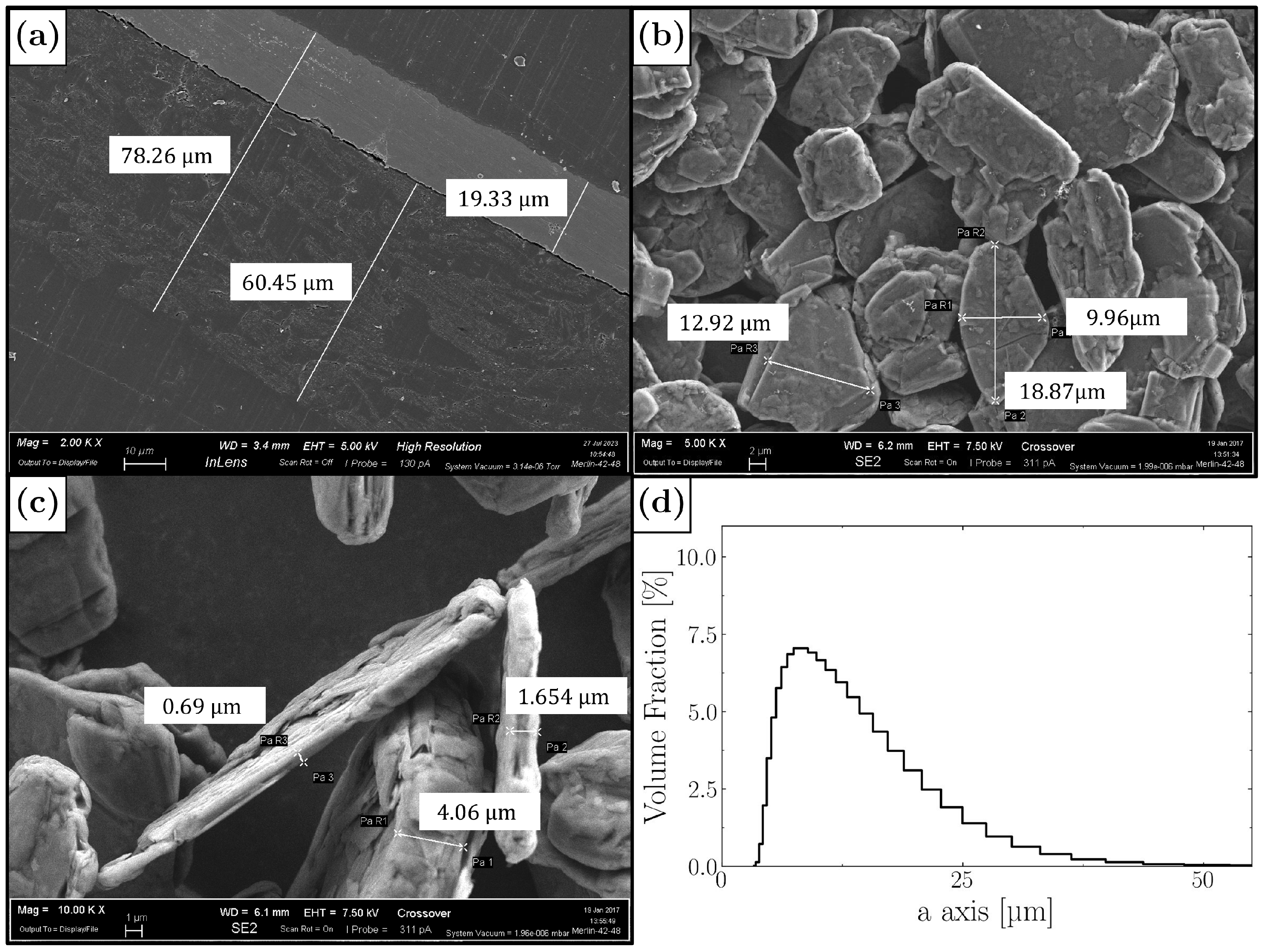
3.1. Experimental Analysis

The experimental electrodes produced in this work were used not only for the determination of the discharge curves but also for the evaluation of the apparent diffusion coefficient within the active material particles and for the estimation of the experimental porosity from FESEM images. The electrodes were manufactured by using a roll-to-roll coating process on commercial Cu metal foils (Schlenk®, Nuremberg, Germany). The anode slurry was prepared by mixing 96.5 wt% of the active material (synthetic graphite, TIMREX SLS30, crystallinity Lc: 200 nm, specific surface area: 6.8 m2 g−1, interlayer distance: 0.3357 nm, Imerys Graphite & Carbon, Bodio, Switzerland), 0.5 wt% of conductive carbon black (TIMCAL C-NERGY™ Super C45, Imerys Graphite & Carbon, Bodio, Switzerland), 1 wt% of sodium carboxymethyl cellulose (Na-CMC 2200, DAICEL Corporation, Osaka, Japan), and 2 wt% of styrene-butadiene rubber (SBR, TRD 102A, JSR Micro N.V., Leuven, Belgium). After solvent removal, electrode disks with an area of 1.766 cm2 and a mass loading of 5.3 mg/cm2 were punched out, vacuum-dried at 120 °C for 4 h (Büchi Glass Oven B-585), and then transferred into an argon-filled glovebox (MBraun Labstar, Garching, Germany, H2O and O2 content < 1 ppm) for cell assembly. Electrochemical performance evaluation was conducted in a half cell configuration (Coin cells 2032) by using lithium discs (Ø 16 mm, 0.6 mm thick, MTI Corporation, Richmond, California, CA, USA) as counter electrodes. All electrochemical tests were performed at room temperature by using an Arbin BT-2000 battery tester (Arbin Instruments, College Station, TX, USA) within the voltage range of 0.01–2 V vs. Li/Li+. Charge/discharge rates were calculated based on the theoretical specific capacity of graphite (375 mAh g−1). The apparent diffusion coefficient was experimentally evaluated with a specific analysis called Galvanostatic Intermittent Titration Technique (GITT) [40,41,42,43]. This test consists of intermittent discharge pulse at a low current value (with a C r a t e = C / 20 ), alternated by relaxation times, as illustrated in Figure 3. Two values of potential difference could be extracted from each current pulse: Δ E t , which is the potential change for the discharge pulse, and  Δ E s , which is the steady state voltage change after eliminating the voltage drop originating from the electrical internal resistance. From these, and applying Equation (12), we could obtain the diffusion coefficient in the electrode as a function of the SoC:
D s = 4 π t p m s V M s M s A s 2 Δ E s Δ E t 2 ,
where m s , V M s , M s , and  A s are, respectively, the mass, the molar volume, the molar mass, and the surface, all referring to the active material. Instead, t p is the pulse time, which for the case under examination was equal to 900 s and is a third of the rest period. In this work, we considered a constant value calculated as the average for the diffusion coefficient to decrease the computational cost of the simulations, but the code we developed is open to also take into account a dynamic diffusion coefficient, dependent on the state of charge.
Morphological analysis of the electrodes was performed using (FESEM) Zeiss SUPRA 40 (ZEISS, Oberkochen, Germany)equipped with a Gemini column and Schottky field emission source (W at 1800 K). Electrode porosity was evaluated by extracting the pore network from FESEM cross-sectional micrographs [44,45].

3.2. The Creation of the Geometry of the Electrodes

In this section, we will illustrate the principal steps of the geometry generation. We would like to specify that the geometry considered is static during the discharge process since we are not considering thermal-mechanical effects that can modify the electrode morphology, especially during charge–discharge fast cycling. Electrodes have been recreated by Discrete Element Method (DEM) simulations using the periodic compression routine implemented in the open-source code Yade [38] (version 2022.01a) coupled with the open-source software Blender [39] (version 4.3.2). The choice of these two pieces of software comes from several reasons: first of all, both of them have a Python API (version 3.10.4) that helped us to produce different geometries in a very simple and automatic way. Moreover, the coupling gives us the possibility to produce particles with complex geometries relatively fast. Below, we describe the workflow for the geometry reconstruction and some notions about DEM simulations. To produce a polydispersed particle packing, with shapes other than spherical, we need a Particle Size Distribution (PSD) and an Aspect Ratio (AR) that in this case is assumed to be constant. The PSD allows us to produce a packing of particles with different sizes; instead, the AR permits us to transform each sphere into an ellipsoid. Firstly, FESEM images of graphite electrodes were obtained. Then, the characteristic lengths of the particles were determined. We noticed that graphite particles are flake-shaped, with one size smaller than the other two, and for this reason, we tried to model them through flattened ellipsoids. Each ellipsoid is characterized by the three semi-axes a, b, c, with  a > b > > c . The thickness, equal to 2 c , is instead kept fixed ( c = 1.5 [µm]). This value was chosen close to the average thickness measured from the available FESEM images. Local variations in the thickness of the graphite flakes would influence the charge and mass transport: in this study we chose to represent this geometric variations by representing the flakes as ellipsoidal shapes, whose thickness varies along their other two main axes (a and b). Furthermore, the open-source code we developed and used to generate the geometries and set up the simulations is capable of considering a distribution of thicknesses, should such data become available. The major axis is taken from the experimental PSD, and the minor axis is calculated from the A R = a / b . In our case, the PSD comes out from an experimental analysis performed in our laboratory [46]; instead, the AR was calculated as an average from FESEM images. Once the input data have been collected, it is possible to run a DEM simulation that can produce a stable and realistic packing of particles. The PSD is the input for Yade, which produces in turn a box of spheres, each of them characterized by a radius equal to the major axis of the future ellipsoidal particle. This setting is fundamental to avoid particle–particle interpenetration in the next step. Therefore, from Yade, we characterize each particle with three spatial coordinates and one radius, and these parameters will become, with the AR, the input for Blender. Here, we can replace each sphere with a different shape, an ellipsoid in this case, so that it is inscribed in the sphere itself. The ellipsoids are initially placed aligning the shorter axes (c) with the fall direction. With this choice, we want to emulate the calendering process. During this operation, graphite particles are compressed to increase the volume density, and, due to the lamellar conformation, they tend to orient themselves parallel to the surface of the current collector. Finally, we can run another DEM simulation on Blender to increase the compaction of the particle bed by finalizing the particle sedimentation process. Now, from Blender, we characterize each particle with nine degrees of freedom: three for the center position, three for the dimensions, and three for the rotation around the axes, and these are the geometrical input parameters for COMSOL Multiphysics 6.1. The script takes as input the geometrical and the physical parameters. In the first group there is the spatial characterization of each particle and the dimensions of the half cell: the thickness and width of both electrode and separator. The physical parameters concern everything that is a material property, like equilibrium potential, diffusion coefficient, electrical conductivity, and so on. Therefore, the Java code works in the following way. First of all, the particles and a central block are generated. In order to facilitate the meshing algorithm in the construction of the grid in the area close to the contact point between two adjacent particles, each of them is enlarged by 1% in each dimension to ensure and improve the contact points. Then, all the particles, or the portion of them, that are outside the block or that are not in touch with the central core of particles are eliminated. The particle fragments fluctuating and not connected with the electrode would lead to an error in the simulation, and therefore, their removal is necessary. After this, the separator is placed in the upper part, and all the domains and surfaces are named to associate each of them with the corresponding material and the physics that will be solved in that zone. Finally, the domain is meshed. The number of elements goes from 180,000 to 300,000 depending on the complexity of the system, and this is the result of the good compromise between low computational cost and high accuracy of the simulation results. In this study we wanted to focus our attention on three systems with different morphology and an increased complexity of the geometry. The simplest electrode has spherical monodispersed particles, the second one has spherical polydispersed particles, and the most complex has flattened ellipsoids to reproduce in a better way the realistic shape of graphite particles. The system with polydispersed spheres was built considering particles with a volume equal to those in the model with ellipsoidal particles. The most simple model, with a package of monodispersed spheres, was instead built considering an average radius calculated from the system of polydispersed spheres. From each half cell, the discharge curve and the concentration of intercalated lithium in the active material were analyzed and compared. It is important to specify that, since we simulated a half cell, the graphite was treated as a cathode, and therefore during discharge, lithium diffused from the electrolyte to the active material particle, and so the concentration of lithium increased during the discharge. The half cells were produced with a thickness of 60 [µm] for the electrode plus 20 [µm] for the separator. To obtain a good characterization of the system, the electrodes had a width of 20 [µm] along the X and Y axes, and the discharges were performed at different current values. The electrode and separator thicknesses were taken from FESEM images, and the width value was obtained from an REV (Representative Elementary Volume) analysis performed both physically (discharge curves) and geometrically (porosity and specific surface), as shown in Figure 4. Among the two geometrical features, porosity is the easiest to compare with experimental evaluation. Nonetheless, the most meaningful insights come from the active material–electrolyte interface within the electrode, as this directly affects lithium-ion transport and intercalation kinetics. At the end of the analysis, we chose to perform our simulations on a domain with a length of 25 [µm].

3.3. DEM Simulation

The initial condition of the DEM simulations is a cloud of non-overlapping spheres, subjected to a vertical force along the z-axis comparable to gravity. Given this external force, the DEM code computes the interaction forces between the spheres and integrates the motion equation for each sphere. The code starts reading the position of a certain sphere, x P ( t ) , and then it calculates the new position at time t + Δ t , integrating Newton’s second law for translation and rotation:
m P d 2 x d t 2 = i = 0 n C ( F i , P N + F i , P T ) + m P g ,
I P d ω d t = i = 0 n C ( F i , P T × d P ( n ) ) ,
where F i , P T and F i , P N are the shear and normal components of the contact force between the two spheres considered for the calculation, respectively. The vertical component is calculated as the product between the article mass ( m P ) and the gravitational acceleration constant ( g ). In the second equation, I P is the moment of inertia and ω is the angular velocity. d P is the distance between the contact point and the center of the particle, and  n is the contact plane normal. Finally, n C is the number of contact points. The interaction between two neighboring particles is modeled by a non-cohesive elastic-frictional contact model [47]. In this modeling approach, the contact force between two spheres can be calculated as the sum of two contributions: the normal component and the shear component. The particles are allowed to overlap at the contact point depending on the Young modulus of the materials. The normal force is calculated from a difference in linear velocity along the interaction axis:
F n = 2 E i r i E j r j E i r i + E j r j u n ,
where u n is the normal displacement and E is the Young modulus of i and j particles’ materials and r i and r j are the radii of particles i and j . In the present work, we considered a unique material for all the interacting particles, and then E i = E j for any i and j particles. The model does not consider long-distance interactions, so when u N 0 , the normal force is null. The shear force comes from the perpendicular component of the linear velocity difference and the perpendicular component of the rotational velocity summation:
F T = K T u T ,
where K T is a function of K N according to Poisson’s law. In this work, the materials’ properties are not modified from Yade’s default. The Blender simulation is similar to the previous one since it also solves Newton’s equations of motion for a system of N particles due to the implementation of the Bullet Physics Library (BPL) [48], which can take into account the collision and interaction between particles in a rigid-body simulation [49].

4. Results and Discussion

The focus of this paper is on the development of a computational workflow aimed at the study of the operational behavior of a lithium ion battery. We focus in particular on the effect of different geometrical shapes on the particles constituting the anode to observe the impact of the electrode morphology in the discharge process. The three systems analyzed are (A) monodispersed spheres, (B) polydispersed spheres, and (C) polydispersed ellipsoids. For each system, the discharge curve and the concentration of intercalated lithium were analyzed, also considering the effect of different initial conditions. In particular, we considered three different discharge rates: C/10, C/5, and C/3. This step, the generation of the model of the electrode geometry, is the point in this workflow where experimental data can most effectively inform the computational model. In this case, the PSD was obtained from image analysis of FESEM scans: an alternative could be to obtain the whole PSD directly via static light scattering. Moreover, with a scanning electron microscope, it is possible to obtain more information about particle morphology, giving the opportunity to create electrodes composed by particles with different shapes. In order to have a good validation of the model analyzed, the discharge curves have been compared with an experimental one obtained in our laboratory. The experimental discharges were made with a current value so as to complete the process in 10 h. Therefore, the comparison is performed only with the model discharged at C/10. This hypothesis is necessary for one important reason: discharge cycles at a higher C-rate would show a marked effect of the polarization phenomena, due to an higher internal resistance, that are not taken into account in the present work. The main operating conditions and geometrical features are summarized in Table 1. The physical coefficients reported for the liquid phase are averaged values, since they are function of the lithium-ion concentration and the complete curve is available in the script itself. Table 2 compares the average porosity of the anode measured experimentally from three independent experiments (affected by an experimental error of approximately 10%) with the values obtained from the three digital replicas. We would like to underline again that the porosity values were evaluated from 2D FESEM images, as previously reported at the end of Section 3.1. As it can be seen, both the polydispersed ellipsoids and the polydispersed spheres fall within the experimental range, with the porosity of the monodispersed spheres replica falling outside of this range. Nonetheless, given the numerical dispersion of the experimental data, from this porosity evaluation both polydispersed spheres and ellipsoids would result in geometrically fitting models. Significantly different are instead the resulting computational specific surface, calculated as the ratio between the solid–liquid interface area and the electrode volume, and the tortuosity, evaluated by the TauFactor algorithm on Matlab R2025a [50], in the separator–current collector direction. We did not report any experimental value for a comparison since the common specific surface data available for commercial graphite particles, already reported in Section 3.1, considers the internal channel connection, which is not directly accessible or represented in the computational model developed in COMSOL. As a result, the computational values in Table 2 are significantly lower than the experimental values. As it will be shown later, the latter choice will prove more accurate from a physical evaluation standpoint.
What can be already be inferred from these preliminary results is that using a simplified model considering spherical shapes of uniform size for the particles results in an electrode that has very different characteristics from the real one. After these considerations regarding the pure geometrical aspect of the electrodes, we can look at the physical behaviors. In the following figures, the continuous red line will represent the system with ellipsoidal particles, the blue dashed dot line will refer to the electrode with polydispersed spheres, the green dashed line to the system formed by monodispersed particles, and the black dotted line will refer to the experimental discharge curve. For a better visualization, we chose a double-logarithm plot to show the results. Indeed, this representation highlights the different stages of graphite lithiation. First of all, the discharge curves at C-rate = C / 10 were compared with an experimental curve obtained in our laboratory. The experimental curve was obtained from the first discharge cycle of a coin cell. In this way, and also due to the low current value, we could neglect degradation effects. Figure 5 shows that the three systems analyzed reproduce the experimental discharge curve reasonably well. This result has two important implications: first, it serves as a second confirmation, after the geometrical analysis in Table 2, that the three generated electrodes are similar and comparable in structure. Second, it suggests that the morphology has a limited impact on the discharge behavior when the current is low. To further quantify the deviation between the experimental discharge curve and the computational predictions, we calculated the root mean square error (RMSE) using Equation (17):
RMSE = i = 1 N ( y m o d e l , i y e x p e r i m e n t , i ) 2
where y m o d e l , i and y e x p e r i m e n t , i represent the simulated and experimental data points, respectively. Table 3 reports the RMSE values for the three systems. Although the system with ellipsoidal particles shows a slightly higher RMSE (0.3861) compared to the monodispersed (0.3638) and polydispersed (0.3046) spherical systems, the differences are moderate and do not compromise the main conclusions of this work. The use of a double-logarithmic scale in Figure 5 was intentionally chosen to emphasize these differences, highlighting the superior representativeness of the ellipsoidal geometry in replicating the actual discharge behavior of the system.
If we apply an higher value of the electric current, moving to higher C-rates, we start to see some differences.
In particular, from Figure 6, we can immediately notice that an increase in the C-rate value leads to an increment in the difference between the curves.
If we want to go more into detail, when C-rate = C / 10 the three curves are almost overlapping, even if there is a small difference between the polydispersed system and the other two. If we look at cases (b) and (c), where C-rate = C / 5 and C-rate = C / 3 , respectively, the curve of monodispersed spheres also begins to diverge from the electrode with ellipsoidal particles, and this difference is more appreciable close to the graphite lithiation state changes, occurring at the points with a visually evident change in slope of the curves. The biggest differences appear when we have a current value such as C-rate = 1 C . Now, the system with monodispersed particles also starts to diverge from the system with ellipsoids, in particular at the end of the discharge process. To better notice the differences between the three morphologies analyzed, we can look at the concentration behavior reported in Figure 7. The contour plots are taken at half of the discharge time, so when SoC = 0.5, and in each row, the half cells are discharged at the same C-rate value.
As is shown by the figure, even if the three systems are at the same total lithiation level, the local concentration of lithium is very different. When the discharge current is low (first row), the vertical gradient of concentration in the electrode is almost null in all the systems. In any case, it is easy to notice that the half cell with ellipsoids reaches concentration values quite higher close to the separator, and the concentration field is more or less constant. On the other hand, the spherical polydispersed system has a negligible concentration gradient along the Z direction, but there is a small radial gradient within the biggest particles. If we look at the second row, in which the current value is such that discharge occurs in 5 h, the differences explained above are more evident. The first half cell shows a marked vertical gradient. Instead, the second system starts to show a vertical gradient of concentration, but also the radial one is increased. The electrode with monodispersed particles does not show almost any difference from the previous case: even if the discharge current value is double, the concentration gradient value is close to zero as in the previous case. When we move to the third row, with a C-rate = C / 3 , the anode made of ellipsoidal particles exhibits a strong gradient from top to bottom, but one important consideration is related to the radial gradient, which is practically null. By contrast, the second electrode shows a very evident radial gradient as well as a vertical gradient. Finally, the electrode with monodispersed particles continues showing a null gradient, both radial and vertical. The last row, with C-rate = 1 C , better underlines the consideration carried out for the previous case. Now, the applied current value is so high that the system with monodispersed spheres also shows a vertical gradient of concentration. Furthermore, the radial gradient in the biggest spherical particle in case (k) is more evident. Looking at system (j) with ellipsoidal particles, it is clear that the vertical gradient is extremely evident, along with the concentration behavior that varies a lot along the separator–current collector direction.
The presence of the vertical gradient, widely observed with X-ray analysis [51], is caused by the increased tortuosity within the electrodes, which is effectively higher for configurations with ellipsoidal particles, as shown in Table 2. The ellipsoidal particles, due to their elongated shape, create a more complex network of pathways through the electrolyte, forcing lithium ions to take longer paths compared to systems with spherical particles. This geometric constraint leads to a reduction in the effective diffusivity in the electrolyte phase and contributes to the observed vertical gradient in concentration.
The anode made of spheres, both monodispersed and polydispersed, offers a lower hindrance, and for this, the local lithiation is almost homogeneous. This clearly demonstrates that only considering polydispersed ellipsoidal particles can result in a realistic representation of electrodes. We can therefore infer that the local and instant concentration profiles of intercalated lithium in the electrode, of lithium in the electrolyte, and, therefore, of lithium at the electrode–electrolyte interface, are more accurately predicted only with a realistic anode (or electrode in general) geometrical representation. Since all irreversible degradation phenomena occur locally and depend on local concentrations, only such computational models can accurately describe them. These phenomena, and the SEI formation in particular, will be the focus of our future work.

5. Conclusions

This study has addressed the limitations of traditional lithium-ion battery modeling, particularly highlighting the importance of accurate electrode geometrical representation. We examined the differences between conventional spherical approximations and the actual shapes of graphite particles, demonstrating that the anisotropic geometry of graphite significantly affects the electrochemical behavior of batteries. By using FESEM images and electrochemical half cell battery models, we were able to show how a precise representation of graphite particles improves the understanding of intra-particle lithiation processes. Additionally, we developed an automatic script to replicate electrodes with various physical and geometric properties, allowing for detailed comparisons between different types of graphite and different geometric configurations. The results highlight that adopting geometrically accurate models can not only improve battery performance predictions but also optimize the study for their design for greater efficiency and longevity. Geometry directly influences the particle arrangements, the porosity, and the specific surface, which has a fundamental importance in an electrochemical model governed by a superficial reaction. The altered ion distribution causes local variations in reaction rates across the electrode, even under uniform current conditions. In contrast, the spherical-particle model promotes more isotropic transport properties and more uniform electrochemical reactions, leading to a flatter lithium concentration profile. This work paves the way for further research on the influence of electrode morphology and supports the idea that increased attention to particle geometry can lead to significant advancements in LiB technology. Ultimately, improved models that consider the true geometries of electrodes could play a crucial role in the evolution of LiBs, significantly contributing to the achievement of global energy sustainability goals. This paper aims to accurately represent the physical and morphological characteristics of LiB electrodes. There are numerous and diverse possibilities for future development in this field, starting from the simplifying assumptions that we have adopted for the present study. Specifically, the use of idealized particle geometries, with a smooth shape or a fixed maximum thickness, simplifies the highly irregular and rough morphology of real graphite particles. Furthermore, our simulations do not incorporate electrochemical degradation mechanisms such as SEI formation or lithium plating, which can play a significant role during long-term cycling. We also neglect thermal effects and mechanical rearrangement that may arise in fast charge and very high inner current values. Future work should aim to address these limitations by incorporating realistic particle shapes, electrochemical aging phenomena, like SEI formation and growth, and thermal effects into the simulation framework. Exploring these phenomena with a too-approximate geometry would lead to a useless simulation that could not help in the design of new batteries. This would provide a deeper understanding of the wear and tear processes that affect battery performance over time. Additionally, incorporating thermal effects into the models could offer insights into how temperature variations impact the efficiency and longevity of the batteries. By pursuing these lines of research, we can further highlight the necessity of precise in silico representations. Such detailed models are crucial for comprehensively understanding the complex interactions between the various physical phenomena occurring within LiBs. These advancements could lead to significant improvements in battery design, performance, and safety, ultimately contributing to the development of more reliable and efficient energy storage systems.

Reproducibility and Data FAIRness

The model to simulate a half cell lithium-ion battery requires few inputs. Starting from the geometrical data, the model needs a particle characterization, which indicates the dimension, position, and rotation values of each particle in each direction for a total of nine degrees of freedom per particle. If the particles are spherical, the number of degrees of freedom reduces to four (three positions and one radius). Moreover, the dimension of the half cell should be provided. These are the electrode and separator thickness and the extension of the simulated battery in the other two directions. Among the physical parameters, the model requires the diffusivity and electrical conductivity values in both liquid and solid phases, and these can be constants or functions of the SoC. Furthermore, there are other parameters required: the electron transfer number, the mean molar activity, and the temperature. Finally, the equilibrium potential of the material of interest, the function of the SoC, has to be provided. The initial conditions needed are the initial SoC, and the current, or the current flow, at the solid–current collector interface. The outputs of the simulation are the intercalated lithium concentration in the solid particles, the lithium-ion concentration in the liquid phase, and the electric potential in both the electrode and electrolyte.
The source code for the generation of the geometry of the electrode is found at the Github repository https://github.com/mulmopro/yade-ellipsoids (accessed on 1 June 2025).
The source code for the setup of the COMSOL simulation, written in the Java COMSOL API format, is found at the Github repository https://github.com/mulmopro/battery_porescale/tree/6.1 (accessed on 1 June 2025) (direct link to the relevant branch, 6.1).
All data presented in this paper, for both tabular and graphical forms, are also available: input data, experimental data used both for model input and validation, and simulation results. This data is found at the Zenodo repository https://zenodo.org/records/14931656 (accessed on 1 June 2025).

Author Contributions

Conceptualization, A.L.P., G.B., and D.M.; methodology, A.L.P. and A.M.; software, A.L.P.; validation, D.V.; formal analysis, A.L.P.; investigation, A.L.P.; resources, D.M.; data curation, A.L.P. and G.B.; writing—original draft preparation, A.L.P.; writing—review and editing, A.M., D.M., and G.B.; visualization, A.L.P. and A.M.; supervision, A.M., D.M., and G.B.; project administration, D.M.; funding acquisition, D.M. All authors have read and agreed to the published version of the manuscript.

Funding

This research was funded by the large-scale European research initiative Battery 2030+ (under grant agreement no. 957213) and the Battery Interface Genome—Materials Acceleration Platform project (www.big-map.eu, under grant agreement no. 957189). This work was funded by the European Commission within the Horizon Europe research and innovation programme (BatCat, under grant agreement no. 101137725). The authors also acknowledge the financial support from ICSC (Centro Nazionale di Ricerca in High Performance Computing, Big Data and Quantum Computing, funded by the European Union—NextGenerationEU).

Data Availability Statement

The original contributions presented in the study are included in the article, further inquiries can be directed to the corresponding author.

Acknowledgments

The authors would like to thank Andrea Querio, Elisa Buccafusco, and Antonio Buffo for the helpful discussion during the work preparation.

Conflicts of Interest

The authors declare no conflicts of interest. The founders had no role in the design of the study; in the collection, analyses, or interpretation of data; in the writing of the manuscript; or in the decision to publish the results.

Nomenclature

TTemperature
FFaraday constant
RIdeal gas constant
ϕ Electric potential
cConcentration
VVolume
( . ) s Referred to solid phase
( . ) Referred to liquid phase
( . ) a Referred to anode side
( . ) c Referred to cathode side
( . ) cc Referred to current collector
( . ) P Referred to a solid particle
( . ) x % Referred to x % of the state of charge
( . ) 0 Initial condition
( . ) ref Reference value
( . ) max Maximum value considered
( . ) min Minimum value considered
iElectric current
K Electrical conductivity
D Diffusion coefficient
tTime
f ± Mean molar activity
t + Lithium-ion transference number
ASurface area
η Over-potential
mMass
MMolar mass
F Force
x Spatial position
I Inertia
g Gravitational acceleration
ω Angular velocity
d Distance
E Young module
r Radius

References

  1. Ziemann, S.; Müller, D.B.; Schebek, L.; Weil, M. Modeling the potential impact of lithium recycling from EV batteries on lithium demand: A dynamic MFA approach. Resour. Conserv. Recycl. 2018, 133, 76–85. [Google Scholar] [CrossRef]
  2. Zhao, Y.; Pohl, O.; Bhatt, A.; Collis, G.; Mahon, P.; Rüther, T.; Hollenkamp, A. A Review on Battery Market Trends, Second-Life Reuse, and Recycling. Sustain. Chem. 2021, 2, 167–205. [Google Scholar] [CrossRef]
  3. Xu, C.; Dai, Q.; Gaines, L.; Hu, M.; Tukker, A.; Steubing, B. Future material demand for automotive lithium-based batteries. Commun. Mater. 2020, 1, 99. [Google Scholar] [CrossRef]
  4. Li, H. Practical Evaluation of Li-Ion Batteries. Joule 2019, 3, 911–914. [Google Scholar] [CrossRef]
  5. Lu, X.; Bertei, A.; Finegan, D.P.; Tan, C.; Daemi, S.R.; Weaving, J.S.; O’Regan, K.B.; Heenan, T.M.M.; Hinds, G.; Kendrick, E.; et al. 3D microstructure design of lithium-ion battery electrodes assisted by X-ray nano-computed tomography and modelling. Nat. Commun. 2020, 11, 2079. [Google Scholar] [CrossRef]
  6. Gupta, A.; Manthiram, A. Designing Advanced Lithium-Based Batteries for Low-Temperature Conditions. Adv. Energy Mater. 2020, 10, 2001972. [Google Scholar] [CrossRef]
  7. Thompson, D.; Hartley, J.; Lambert, S.; Shiref, M.; Harper, G.; Kendrick, E.; Anderson, P.; Ryder, K.; Gaines, L.; Abbott, A. The importance of design in lithium ion battery recycling—A critical review. RSC Green Chem. 2020, 22, 7585–7603. [Google Scholar] [CrossRef]
  8. Doyle, M.; Fuller, T.F.; Newman, J. The importance of the lithium ion transference number in lithium/polymer cells. Electrochim. Acta 1994, 39, 2073–2081. [Google Scholar] [CrossRef]
  9. Doyle, M.; Fuller, T.F.; Newman, J. Modeling of Galvanostatic Charge and Discharge of the Lithium/Polymer/Insertion Cell. J. Electrochem. Soc. 1993, 140, 1526. [Google Scholar] [CrossRef]
  10. Jokar, A.; Rajabloo, B.; Désilets, M.; Lacroix, M. Review of simplified Pseudo-two-Dimensional models of lithium-ion batteries. J. Power Sources 2016, 327, 44–55. [Google Scholar] [CrossRef]
  11. Qiu, G.; Dennison, C.; Knehr, K.; Kumbur, E.; Sun, Y. Pore-scale analysis of effects of electrode morphology and electrolyte flow conditions on performance of vanadium redox flow batteries. J. Power Sources 2012, 219, 223–234. [Google Scholar] [CrossRef]
  12. Chung, D.D.L. Review Graphite. J. Mater. Sci. 2002, 37, 1475–1489. [Google Scholar] [CrossRef]
  13. Deprez, N.; McLachlan, D.S. The analysis of the electrical conductivity of graphite conductivity of graphite powders during compaction. J. Phys. D Appl. Phys. 1988, 21, 101. [Google Scholar] [CrossRef]
  14. Gottschalk, L.; Müller, J.; Schoo, A.; Baasch, E.; Kwade, A. Spherical Graphite Anodes: Influence of Particle Size Distribution and Multilayer Structuring in Lithium-Ion Battery Cells. Batteries 2024, 10, 40. [Google Scholar] [CrossRef]
  15. Bläubaum, L.; Röder, F.; Nowak, C.; Chan, H.S.; Kwade, A.; Krewer, U. Impact of Particle Size Distribution on Performance of Lithium-Ion Batteries. ChemElectroChem 2020, 7, 4755–4766. [Google Scholar] [CrossRef]
  16. Yu, H.; Zhang, L.; Wang, W.; Yang, K.; Zhang, Z.; Liang, X.; Chen, S.; Yang, S.; Li, J.; Liu, X. Lithium-ion battery multi-scale modeling coupled with simplified electrochemical model and kinetic Monte Carlo model. iScience 2023, 26, 107661. [Google Scholar] [CrossRef]
  17. Lu, X.; Lagnoni, M.; Bertei, A.; Das, S.; Owen, R.E.; Li, Q.; O’Regan, K.; Wade, A.; Finegan, D.P.; Kendrick, E.; et al. Multiscale dynamics of charging and plating in graphite electrodes coupling operando microscopy and phase-field modelling. Nat. Commun. 2023, 14, 5127. [Google Scholar] [CrossRef] [PubMed]
  18. Danner, T.; Singh, M.; Hein, S.; Kaiser, J.; Hahn, H.; Latz, A. Thick electrodes for Li-ion batteries: A model based analysis. J. Power Sources 2016, 334, 191–201. [Google Scholar] [CrossRef]
  19. Westhoff, D.; Manke, I.; Schmidt, V. Generation of virtual lithium-ion battery electrode microstructures based on spatial stochastic modeling. Comput. Mater. Sci. 2018, 151, 53–64. [Google Scholar] [CrossRef]
  20. Kremer, L.S.; Hoffmann, A.; Danner, T.; Hein, S.; Prifling, B.; Westhoff, D.; Dreer, C.; Latz, A.; Schmidt, V.; Wohlfahrt-Mehrens, M. Manufacturing Process for Improved Ultra-Thick Cathodes in High-Energy Lithium-Ion Batteries. Energy Technol. 2020, 8, 1900167. [Google Scholar] [CrossRef]
  21. Hein, S.; Danner, T.; Westhoff, D.; Prifling, B.; Scurtu, R.; Kremer, L.; Hoffmann, A.; Hilger, A.; Osenberg, M.; Manke, I.; et al. Influence of Conductive Additives and Binder on the Impedance of Lithium-Ion Battery Electrodes: Effect of Morphology. J. Electrochem. Soc. 2020, 167, 013546. [Google Scholar] [CrossRef]
  22. Deng, Z.; Lin, X.; Huang, Z.; Meng, J.; Zhong, Y.; Ma, G.; Zhou, Y.; Shen, Y.; Ding, H.; Huang, Y. Recent progress on advanced imaging techniques for lithium-ion batteries. Adv. Energy Mater. 2021, 11, 2000806. [Google Scholar] [CrossRef]
  23. An, S.J.; Li, J.; Daniel, C.; Mohanty, D.; Nagpure, S.; Wood, D.L. The state of understanding of the lithium-ion-battery graphite solid electrolyte interphase (SEI) and its relationship to formation cycling. Carbon 2016, 105, 52–76. [Google Scholar] [CrossRef]
  24. Chouchane, M.; Arcelus, O.; Franco, A.A. Heterogeneous Solid-Electrolyte Interphase in Graphite Electrodes Assessed by 4D-Resolved Computational Simulations. Batter. Supercaps 2021, 4, 1457–1463. [Google Scholar] [CrossRef]
  25. Pron, V.; Versaci, D.; Amici, J.; Francia, C.; Santarelli, M.; Bodoardo, S. Electrochemical Characterization and Solid Electrolyte Interface Modeling of LiNi 0.5 Mn 1.5 O 4 -Graphite Cells. J. Electrochem. Soc. 2019, 166, A2255–A2263. [Google Scholar] [CrossRef]
  26. Heiskanen, S.K.; Kim, J.; Lucht, B.L. Generation and Evolution of the Solid Electrolyte Interphase of Lithium-Ion Batteries. Joule 2019, 3, 2322–2333. [Google Scholar] [CrossRef]
  27. Peled, E.; Menkin, S. Review—SEI: Past, Present and Future. J. Electrochem. Soc. 2017, 164, A1703. [Google Scholar] [CrossRef]
  28. Nie, M.; Lucht, B.L. Role of Lithium Salt on Solid Electrolyte Interface (SEI) Formation and Structure in Lithium Ion Batteries. J. Electrochem. Soc. 2014, 161, A1001. [Google Scholar] [CrossRef]
  29. Keil, P.; Schuster, S.F.; Wilhelm, J.; Travi, J.; Hauser, A.; Karl, R.C.; Jossen, A. Calendar Aging of Lithium-Ion Batteries. J. Electrochem. Soc. 2016, 163, A1872. [Google Scholar] [CrossRef]
  30. Goldin, G.M.; Colclasure, A.M.; Wiedemann, A.H.; Kee, R.J. Three-dimensional particle-resolved models of Li-ion batteries to assist the evaluation of empirical parameters in one-dimensional models. Electrochim. Acta 2012, 64, 118–129. [Google Scholar] [CrossRef]
  31. Newman, J.; Balsara, N.P. Electrochemical Systems; John Wiley & Sons: Hoboken, NJ, USA, 2021. [Google Scholar]
  32. Latz, A.; Zausch, J. Thermodynamic consistent transport theory of Li-ion batteries. J. Power Sources 2011, 196, 3296–3302. [Google Scholar] [CrossRef]
  33. Richardson, G.W.; Foster, J.M.; Ranom, R.; Please, C.P.; Ramos, A.M. Charge transport modelling of Lithium-ion batteries. Eur. J. Appl. Math. 2022, 33, 983–1031. [Google Scholar] [CrossRef]
  34. Kespe, M.; Nirschl, H. Numerical simulation of lithium-ion battery performance considering electrode microstructure. Int. J. Energy Res. 2015, 39, 2062–2074. [Google Scholar] [CrossRef]
  35. Bard, A.J.; Faulkner, L.R.; White, H.S. Electrochemical Methods: Fundamentals and Applications; John Wiley & Sons: Hoboken, NJ, USA, 2022. [Google Scholar]
  36. Colclasure, A.M.; Kee, R.J. Thermodynamically consistent modeling of elementary electrochemistry in lithium-ion batteries. Electrochim. Acta 2010, 55, 8960–8973. [Google Scholar] [CrossRef]
  37. Karthikeyan, D.K.; Sikha, G.; White, R.E. Thermodynamic model development for lithium intercalation electrodes. J. Power Sources 2008, 185, 1398–1407. [Google Scholar] [CrossRef]
  38. Smilauer, V. Yade Documentation; The Yade Project: Lowestoft, UK, 2021; Available online: https://zenodo.org/records/5705394 (accessed on 9 June 2025).
  39. Filippov, S. Blender software platform as an environment for modeling objects and processes of science disciplines. Keldysh Inst. Prepr. 2018, 24, 1–42. [Google Scholar] [CrossRef]
  40. Park, J.H.; Yoon, H.; Cho, Y.; Yoo, C.Y. Investigation of Lithium Ion Diffusion of Graphite Anode by the Galvanostatic Intermittent Titration Technique. Materials 2021, 14, 4683. [Google Scholar] [CrossRef]
  41. Markevich, E.; Levi, M.; Aurbach, D. Comparison between potentiostatic and galvanostatic intermittent titration techniques for determination of chemical diffusion coefficients in ion-insertion electrodes. J. Electroanal. Chem. 2005, 580, 231–237. [Google Scholar] [CrossRef]
  42. Yang, H.; Bang, H.J.; Prakash, J. Evaluation of Electrochemical Interface Area and Lithium Diffusion Coefficient for a Composite Graphite Anode. J. Electrochem. Soc. 2004, 151, A1247. [Google Scholar] [CrossRef]
  43. Horner, J.S.; Whang, G.; Ashby, D.S.; Kolesnichenko, I.V.; Lambert, T.N.; Dunn, B.S.; Talin, A.A.; Roberts, S.A. Electrochemical Modeling of GITT Measurements for Improved Solid-State Diffusion Coefficient Evaluation. ACS Appl. Energy Mater. 2021, 4, 11460–11469. [Google Scholar] [CrossRef]
  44. Rabbani, A.; Salehi, S. Dynamic modeling of the formation damage and mud cake deposition using filtration theories coupled with SEM image processing. J. Nat. Gas Sci. Eng. 2017, 42, 157–168. [Google Scholar] [CrossRef]
  45. Ezeakacha, C.P.; Rabbani, A.; Salehi, S.; Ghalambor, A. Integrated Image Processing and Computational Techniques to Characterize Formation Damage. In Proceedings of the SPE International Conference and Exhibition on Formation Damage Control, Lafayette, LA, USA, 7–9 February 2018; p. D012S007R004. [Google Scholar] [CrossRef]
  46. Castillo, J.; Soria-Fernández, A.; Rodriguez-Peña, S.; Rikarte, J.; Robles-Fernández, A.; Aldalur, I.; Cid, R.; González-Marcos, J.A.; Carrasco, J.; Armand, M.; et al. Graphene-Based Sulfur Cathodes and Dual Salt-Based Sparingly Solvating Electrolytes: A Perfect Marriage for High Performing, Safe, and Long Cycle Life Lithium-Sulfur Prototype Batteries. Adv. Energy Mater. 2024, 14, 2302378. [Google Scholar] [CrossRef]
  47. Cundall, P.A.; Strack, O.D. A discrete numerical model for granular assemblies. Geotechnique 1979, 29, 47–65. [Google Scholar] [CrossRef]
  48. Coumans, E. Bullet physics simulation. In Proceedings of the ACM SIGGRAPH 2015 Courses, Association for Computing Machinery, Los Angeles, CA, USA, 9–13 August 2015. [Google Scholar] [CrossRef]
  49. Boccardo, G.; Augier, F.; Haroun, Y.; Ferré, D.; Marchisio, D.L. Validation of a novel open-source work-flow for the simulation of packed-bed reactors. Chem. Eng. J. 2015, 279, 809–820. [Google Scholar] [CrossRef]
  50. Cooper, S.; Bertei, A.; Shearing, P.; Kilner, J.; Brandon, N. TauFactor: An open-source application for calculating tortuosity factors from tomographic data. SoftwareX 2016, 5, 203–210. [Google Scholar] [CrossRef]
  51. Yao, K.P.C.; Okasinski, J.S.; Kalaga, K.; Shkrob, I.A.; Abraham, D.P. Quantifying lithium concentration gradients in the graphite electrode of Li-ion cells using operando energy dispersive X-ray diffraction. Energy Environ. Sci. 2019, 12, 656–665. [Google Scholar] [CrossRef]
Figure 1. (a) FESEM image of electrode of half cell: graphite and separator. (b) FESEM image of graphite layer. (c) FESEM image of graphite particle. (d) PSD of graphite particles within electrode.
Batteries 11 00252 g001
Figure 2. A schematic representation of the LiB cell with the most relevant equations. The blue dashed line highlights the half cell simulated in this work.
Batteries 11 00252 g002
Figure 3. The Galvanostatic Intermittent Titration Technique. (a) Discharge potential as a function of the time for the complete GITT. (b) The discharge potential as a function of the time for one single pulse. Δ E s (blue) and Δ E t (red) are the two potential differences that appear in the equation that expresses the lithium diffusion coefficient as a function of the SoC. (c) The lithium diffusion coefficient in the active material as a function of the SoC. The red dots are the values obtained from Equation (12). The continuous black line is the interpolation line. The continuous blue line represents the average value.
Batteries 11 00252 g003
Figure 4. (a) Physical REV analysis, discharge curve comparison; (b) geometrical REV analysis, evaluation of porosity and specific surface.
Batteries 11 00252 g004
Figure 5. Discharge curves as a function of the SoC, a comparison between modeling and experimental results. The continuous red line represents the system with ellipsoidal particles, the blue dashed dot line refers to the electrode with polydispersed spheres, the green dashed line alludes to the system formed by monodispersed particles, and the black dotted line refers to the experimental discharge curve.
Batteries 11 00252 g005
Figure 6. Discharge curves as a function of the SoC. The continuous red line represents the system with ellipsoidal particles, the blue dashed dot line refers to the electrode with polydispersed spheres, and the green dashed line to the system formed by monodispersed particles. (a) C-rate = 1 C ; (b) C-rate = C / 5 ; (c) C-rate = C / 3 ; (d) C-rate = C / 10 .
Batteries 11 00252 g006
Figure 7. The local intercalated lithium concentration within the electrode. Images taken at half discharge, SoC = 50%. First row (a,b,c): C-rate = C/10; second row (d,e,f): C-rate = C/5; third row (g,h,i): C-rate = C/3; fourth row (j,k,l): C-rate = 1C. First column (a,d,g,j): ellipsoidal particles; second column (b,e,h,k): polydispersed spherical particles; third column (c,f,i,l): monodispersed spherical particles.
Batteries 11 00252 g007
Table 1. Parameters used in 4D resolved electrochemical model.
ParameterValueDescription
c 0 s 0 [mol/m3]Initial Li concentration in solid
c 0 1000 [mol/m3]Initial Li+ concentration in liquid
c max s 31,507 [mol/m3]Maximum Li concentration in solid
SoC max 0.95Final particle lithiation level
SoC min 0Initial particle lithiation level
K s 100 [S/m]Electrode electrical conductivity
K 0.743 [S/m]Electrolyte electrical conductivity
D s 1.317 × 10 14 [m2/s]Electrode diffusion coefficient
D 3.613 × 10 10 [m2/s]Electrolyte diffusion coefficient
α a 0.5Anodic symmetry factor
α c 0.5Cathodic symmetry factor
t + 0.363Lithium-ion transference number
h min 0.85 [µm]Minimum mesh size
h max 6.6 [µm]Maximum mesh size
Δ x 20 [µm]Electrode thickness along X direction
Δ y 20 [µm]Electrode thickness along Y direction
Δ z 60 [µm]Electrode thickness along Z direction
s e p 20 [µm]Separator thickness
Table 2. The geometrical descriptors of the three types of reconstructed electrodes, compared with the experimental value.
GeometryExp. PorosityComp. PorosityComp. Specific Area [m2/m3]Tortuosity
Monodispersed spheres 0.3769.29 × 10 5 2.05
Polydispersed ellipsoids0.3000.2719.90 × 10 5 7.8
Polydispersed spheres 0.3015.93 × 10 5 2.33
Table 3. The root mean square error for the three simulated discharge curves with respect to the experimental one.
SystemRMSE
Ellipsoidal0.3861
Monodispersed0.3638
Polydispersed0.3046
Disclaimer/Publisher’s Note: The statements, opinions and data contained in all publications are solely those of the individual author(s) and contributor(s) and not of MDPI and/or the editor(s). MDPI and/or the editor(s) disclaim responsibility for any injury to people or property resulting from any ideas, methods, instructions or products referred to in the content.

