1. Introduction
The optimum design of electrical machines and magnetic components requires the use of accurate and performing macroscale hysteresis models, capable of reproducing the evolution of the material magnetization and the prediction of the power losses, under real working conditions. Indeed, in power electronic applications, the magnetic cores are often subjected to distorted supply signals [
1,
2,
3], eventually giving rise to subloops in the main hysteresis cycle [
2] or DC-biased magnetizations, causing asymmetric minor loops [
3]. The most important effects of the harmonics and the DC bias, which negatively influence the performance of the devices, are extra power losses, vibrations, noise, and local heating. Achieving such a detailed knowledge on the material behavior, starting from the limited information usually provided by the manufacturers, is a challenging issue, almost completely mandated to the capabilities of the material model. Accuracy, robustness, and reliability, as well as the possibility of being identified from a minimal set of experimental data, are the most important requisites the hysteresis model has to comply with.
The design of magnetic cores is typically dealt with commercial computer-aided design (CAD) software, based on the finite-element method (FEM), allowing the definition of customized geometries [
4]. However, to correctly model the ferromagnetic material, a hysteretic constitutive law B(H) has to be taken into account [
5,
6,
7]. Hysteretic B(H) characteristics allow a suitable computation of the evolution of the material magnetization and the prediction of the hysteresis losses as a function of the amplitude of the excitation. Indeed, the area enclosed by the B-H loop is the specific energy (per unit of volume) absorbed by the material in one period of excitation. In addition to the aforementioned requisites, to be suitable for applications in finite-element analysis, the hysteresis models must be computationally fast and memory-efficient.
Feedforward neural networks (FFNNs) became quite popular in modeling nonlinear systems, also accounting for vector problems [
8], because they allow a very fast calculation of the output with a reduced occupation of memory. The feedforward architecture is preferred over the others mostly for the abundance of well-established learning algorithms. On the other hand, FFNNs are seldom employed as standalone hysteresis models, since they lack intrinsic past history dependence. In most of the approaches proposed and investigated in the literature, the neural networks are coupled with the Preisach model (PM) [
9,
10,
11], gaining a high accuracy at the expense of computational time and memory allocation. Despite the slow simulation speed, the PM is still now preferred for its accuracy in the replication of hysteresis loops under various types of excitation waveforms and for the relatively easy identification from a minimal amount of measured data [
12,
13,
14,
15].
Other approaches are based on the emulation of the past history dependence via numerical algorithms coupled to the neural net [
16], such as the transplantation method [
17], without noticeably worsening the computational and memory efficiency of the neural net alone. Different architectures, such as recurrent neural networks (RNNs), which have theoretically built-in dependence on the past history, are rarely employed in magnetic hysteresis modeling problems, due to the complexity of the training procedure and the lower availability of learning algorithms [
18,
19].
In this paper, we propose a hysteresis model, with magnetic field
H (A/m) as the input and magnetic induction
B (T) as the output, based on a standalone multilayer feedforward neural network, and we apply it to simulate the magnetization processes of a commercial grain-oriented (GO) electrical steel sheet. Instead of coupling the net with other numerical models or algorithms, the memory dependence is directly embedded in the network, reserving some input neurons for the actual and some past values of both
H and
B. According to this architecture, for a given future value of
H, the neural network is theoretically able to get the correct future value of
B depending on the possible different past values of both
H and
B. Clearly, a suitable training set has to be defined for the considered material, starting from a minimal information on its experimental behavior. A straightforward magnetization process, useful to train our FFNN, consists of major hysteresis loops with equally spaced subloops, uniformly distributed along its ascending and descending branches. The first branch of each subloop is a sector of a first-order reversal curve (FORC), while the closure branch is a sector of a second-order reversal curve (SORC). The inversion points, located at the ascending and descending branches, are reached at two times from two different past values of
H and
B, allowing the FFNN to distinguish the two different future values of the output depending on the past status. A successfully trained network will, therefore, be able to generalize that pattern, allowing the simulation of magnetization processes under distorted excitations. Thermal effects, mostly influencing the magnetic permeability and the saturation magnetization [
20], are not taken into account here. It has already been pointed out that the use of the Preisach model for the generation of the training set is more convenient than the direct training of the FFNN on the experimental loops [
17]. Indeed, a quite large amount of data would be necessary, and the magnetization process itself would be almost complex to measure via conventional equipment, according to standardized procedures. Instead, the PM can be effectively identified using very few symmetric hysteresis loops, which can be either provided by the manufacturer or measured via an Epstein frame, according to IEC 60404-2.
Firstly, the ferromagnetic material was experimentally characterized using the Epstein frame realized in out laboratory. A family of eight quasi-static symmetric hysteresis loops was measured, under a sinusoidal magnetic induction waveform. Then, we selected only three experimental loops to identify the PM, which was successively used to generate the training set described before. The FFNN was trained following an optimized procedure that we implemented in a computer program with a graphical user interface (GUI), written in Matlab®. The resulting neural network (NN)-based model was firstly validated by the reproduction of the remaining measured hysteresis loops, not involved in the identification. The loops simulated by the NN-based model were in this case compared to both those measured and those calculated by the PM. Conclusively, other relevant hysteresis processes were generated by the PM to emulate the typical working excitations to which the ferromagnetic cores are subjected in real applications, such as DC-biased magnetization loops and distorted excitation waveforms. The latter comparative analysis was aimed at testing the capability of the NN-based model in the replication of the results obtained by the PM simulations under an arbitrary excitation field. The possibility to reach a satisfactory degree of accuracy in a wide range of excitations, while saving the computational time and the memory allocation, is an important step toward a future coupling of the hysteresis model with finite-element schemes, for dynamic simulations of magnetic cores.
2. Materials and Methods
The ferromagnetic material examined in this work was a commercial grain-oriented iron–silicon laminated alloy, grade M4T27, suitable for the fabrication of performing cores for transformers, filtering inductors, and innovative electric motors. Grain orientation, in soft magnetic alloys, is achieved via complex fabrication processes, including multistep cold and hot rolling with intermediate annealing [
21,
22]. The final alloy had a typical grain size of few millimeters, and most of the grains were aligned according to the so-called “Goss orientation”. The optimal magnetic properties, such as the permeability in the linear region, the coercive field, and the area of the hysteresis loop, were developed along the rolling direction and, thanks to the high degree of orientation, were almost uniform in the sheet plane. For this reason, the coupling phenomenon of one grain with its neighborhoods could be practically neglected.
The main parameters of the alloy, provided by the manufacturer, are listed in
Table 1.
2.1. Experimental Investigation
An 840-turn, 30 × 30 Epstein circuit, realized in our laboratory in agreement with the international standard IEC60404-2, was used to experimentally characterize the GO steel sheet. The magnetic circuit was realized by assembling eight strips for each side of the device, with double-overlapping joints. The primary coil of the magnetic circuit was supplied by means of a linear, programmable, four-quadrant, signal amplifier, having a maximum output power of 180 W. The current flow on the primary coil, from which the magnetic field is calculated, was detected using an active probe based on the Hall effect, and the voltage applied was also sensed to monitor the measurement process. The magnetic induction of the ferromagnetic material was calculated from the measure of the electromotive force at the secondary coil. A data acquisition module, working in acquisition/generation mode, was used to acquire the signals (primary voltage and current, secondary voltage) and to generate the input voltage signal of the power amplifier. The complete list of equipment constituting the experimental setup is reported in
Table 2.
A PC managed the control and the supervision of the measurement process, thanks to a dedicated computer program, written in Matlab® by the authors. The quasi-static hysteresis loop was obtained as the average over np periods of the measured signals of H(t) and B(t) at a given fundamental frequency f0.
The measure of hysteresis processes requires that the possible dynamic effects, such as those associated with the circulation of the eddy currents, are negligible. For iron-based laminated alloys, it is sufficient to keep the supply frequency below a few Hertz [
6,
13,
14]. A powerful feedback algorithm, described in detail in [
14], was implemented with the aim of controlling the waveform of the magnetic induction, which must be sinusoidal, according to the international standard IEC 60404-2. The effectiveness of the feedback algorithm was expressed in terms of the absolute difference (
MAEAR) between the aspect ratio of the measured signal and that of the pure sinusoidal wave, equal to
. In addition, the maximum value of the mean absolute error (
MAEmax) between the reference waveform and the measured waveform of
B was evaluated to determine the exit condition of the feedback. In addition, the specimen under test was carefully demagnetized before each acquisition, in order to avoid undesired bias values of the magnetic induction, which would lead to an asymmetric hysteresis loop. The parameters set in order to perform the acquisition and the values used in our experimental investigation are illustrated in
Table 3.
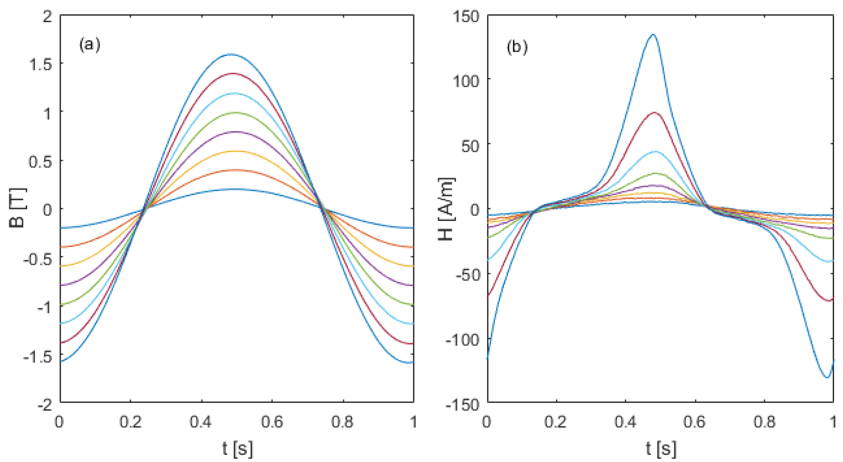
A family of eight quasi-static symmetric loops was measured for the following values of magnetic induction amplitude:
, with
n = 1, …, 8. The measured waveforms of both the
B and the
H fields are displayed in
Figure 1a,b, respectively. As one can see, the waveforms of
B were purely sinusoidal, whilst those of
H were highly distorted.
2.2. Preisach Model Computations
The traditional scalar Preisach model [
23] was identified for the M4T27 steel with the aim of generating a suitable training set for the NN-based model. The core of this model is the Preisach hysteresis operator (also called the Preisach hysteron), which is basically a bistable operator with a unitary output and thresholds
Hup,
Hdown.
The two degrees of freedom that characterize the operator, instead of Hup, Hdown, were equivalently expressed in terms of the interaction field Hi = (Hup + Hdown)/2 and the intrinsic coercivity u = (Hup − Hdown)/2.
The Preisach operators were distributed on the
H field axis, and the analytical expression of the model output was given by a suitable weighted superposition of their contributions,
where
D+ and
D− are the regions of the domain in which the operators have respectively positive (+1) and negative (−1) output, while
P is the weight function.
The numerical implementation of the Preisach model firstly required the definition of two grid vectors:
Hi, representing the nodes on the
H field in which the hysterons are located, and
u, representing the possible values of the coercive field. The length of the two vectors
Hi and
u, are indicated respectively with
NH and
NU, while
Nhyst =
NH⋅
NU is the total number of hysterons. To optimize the computational performances of the model, it is convenient to locate the operators not uniformly with respect to both the interaction field and the coercivity values. Indeed, it is straightforward to increase the density of operators and then the number of Barkhausen jumps, where the magnetic permeability of the material is higher. The following equations were adopted to define the numerical grid of hysterons:
where
.
where
.
After that, the hysteron weight function
P(
Hi,
u) has to be found. To allow the identification from a few symmetric hysteresis loops, it is convenient to approximate the weight function with probability distributions, rather than solving the Everett integral in Equation (1) in the analytic form [
23].
Here, we used the classic Preisach model, which does not account for the reversible component of the magnetization; for this reason, a slightly different formulation of the weight function is proposed. Variable separation was applied to express
P as the product of two distribution functions, one depending only on H
i and the other depending on only
u:
. The first term is given by the linear combination of two Lorentzian functions, while the second term is a single Lorentzian function:
. The expression of
LH1,
LH2, and
LU is described below.
where
are the parameters describing the standard deviations of
L1 and
L2 with respect to
Hi,
describes the standard deviation of
LU with respect to
u, and
u0 is the most probable value of the intrinsic hysteron coercive field.
The magnetization, at the
k-th sample step, is calculated as
where
is the (unitary) magnetization of the
j-th hysteron at the sample step
k.
It has been shown that the Lorentzian function is more adequate than other probability density functions to represent the weight function for Preisach operators [
15,
23].
According to the numerical implementation of the model that we developed, P and qk are column vectors with length Nhyst, while Mk is evaluated as a scalar product. Before the computation of Mk, the column vector qk is determined for the current value of the magnetic field Hk and the previous value qk−1. The model was implemented at a low level of abstraction in a computer program, written in Matlab®.
The model is characterized by (
), which can be identified using experimental data via standard algorithms. It has been shown that very few symmetric measured loops are sufficient to obtain a satisfactory model identification, exploiting a suitable cost function [
15]. Local minima of the cost function in the parameter space can be avoided by means of a preliminary verification stage in the whole computational domain by using a genetic algorithm (GA). The best combination of parameters is, thus, determined, and their values are used as initial point for the successive search of the minimum point of the cost function. This second stage was performed by the pattern search algorithm (PSA). In this work, only three measured hysteresis cycles were taken into account to identify the model, specifically, those having amplitude
B0 = 0.4, 1.0, 1.6 T.
2.3. Neural Network-Based Model
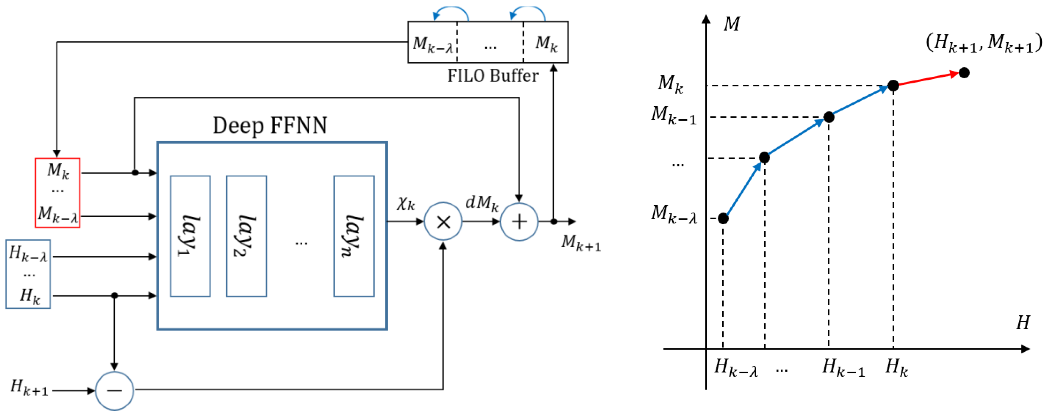
The neural network-based hysteresis model proposed here was based on the architecture shown in
Figure 2. The core of the model was a multilayer feedforward neural network (FFNN) with 2
λ inputs and one output. The input layer consisted of 2
λ neurons with a linear characteristic relation: half of them were reserved for the
λ previous values of the magnetic field, while the other half were reserved for the
λ previous values of the magnetization. By virtue of the feedforward architecture, the input variables were transmitted to all the neurons of the first hidden layer. The characteristic relation of the neurons pertaining to the hidden layers and the output layer is
where
J is the number of neurons in the previous layer,
xj is the output of the
j-th neurons of the previous layer,
wj is the synaptic weight which connects the neuron to the
j-th one of the previous layer,
b is the bias value, and
fact is the neuron activation function.
Except for the neurons of the input and the output layers, which have purely linear characteristics, the activation function is the hyperbolic-tangent sigmoid described below.
A more detailed explanation on the feedforward neural network modeling can be found in [
24].
The output of the FFNN is the current value of the magnetic susceptibility as a function of the λ past values of both the magnetic field and the magnetization, from which the future value of the magnetization Mk+1 can be calculated as . The computation of the model output was performed in a closed-loop configuration, in which the λ past values of M, sent as input at each time step k, were those calculated by the model in the previous steps. For this reason, a first input last output (FILO) buffer was required to store the λ floating-point variables Mk, …, Mk-λ. At each step, the variables stored in the buffer were updated (shifted toward the left) for the computation of the successive value of M. Lastly, let us point out that, since the output of the FFNN is the magnetic susceptibility, the model can be easily inverted, allowing coupling with FEM.
The model is fully described by the vector NPL containing the number of neurons per each hidden layer. The authors implemented the NN-based model at a low level of abstraction via a computer program written in Matlab®. The program consisted of a simple main script (main_simul_NN.m) in which the magnetic field sequence could be either directly defined by the user as a row vector or loaded from a .txt file.
The computation of the output in a closed-loop configuration was performed sample-by-sample in an iterative procedure. At each iteration, the main program calls a Matlab
® function, named “NN_model.m”, to solve the output magnetization. The two files are shared by the authors as
Supplementary Materials. Alternatively, exploiting the Neural Network Toolbox of Matlab
®, it is possible to handle the FFNN at a higher level of abstraction, which can be saved as a structure, with defined fields and methods. The same main program can be used to simulate the neural network at the high level of abstraction, calling the method “sim” (=simulate) of the structure instead of calling the function “NN_model.m” in the iterative procedure. However, as shown in
Section 3, the computational speed is significantly reduced.
2.4. Training Procedure
An optimized training procedure, with multiple verification steps, was developed to determine the network architecture and successively to identify the optimum values of its weights and biases. Traditionally, FFNNs are trained by running a method, such as the Levenber–Marquardt of the scaled-conjugate gradient, for a given number of epochs. The final value of the training error, typically the mean squared error (MSE), and its evolution versus the epochs are taken into account to verify whether the network was successfully trained or not. Since the MSE function has many local minima in the parameter space, it is not possible to know a priori how many times the training method must be run. Furthermore, during the training, the is calculated in an open-loop configuration, while the neural network operates in a closed-loop configuration during simulations. Let us indicate with the mean squared error calculated at the open-loop configuration during the training. As the neural networks with a feedback loop could be numerically unstable, independently of the values of , a suitable stability check is also required.
Here, we verified the numerical stability after the training by the simulation of the same training set in a closed-loop configuration, as well as by a comparison of the obtained mean squared error (
) with
. After the training set was simulated, the area enclosed by the calculated loop on the
H–
B plane was compared to that of the training set. In particular, as the final step of the performance verification, the displacement between the two values of the loop area was taken into account. In order to optimize and speed up the identification of the optimum network, the network training and successive multistep verification of its performance were implemented in an automatic procedure, in which the training method was launched iteratively. At each launch, a number
of epochs are processed, or less if
becomes lower than the threshold
. Then, the training set is simulated and the
is computed. If
is higher than the threshold
, a new iteration starts; otherwise, the area enclosed by the obtained loop is evaluated and the relative displacement
with respect to that of the training set is calculated. The iterative procedure stops if either the area displacement becomes lower than
or the maximum number of iterations is reached. The authors developed a graphical user interface (GUI) to manage the described procedure in an easier and faster way for the end user. The main window of the program is shown in
Figure 3.
The user interface is based on a single window plus eventually some interactive dialog boxes. The window is subdivided into four panels, two of which are located in the upper half. In the uppermost panel, the features and the topology of the neural network have to be set. Notice that in the “neurons per layer” text box, the NPL vector, with comma-separated values, has to be inserted. In the subsequent panel, the user must specify the path of the working folder, the name of the files related to the input and the output of the training set, the training method, the number of epochs, and the threshold value of . In the lower half of the main window, two panels, put side by side, and three push-buttons to start, to pause, and to abort the training, are located. In the “algorithm settings” panel, the user can set the values of , , and the maximum number of iterations. At each iteration, if the values of and are smaller than any of those obtained at the previous iterations, the currently trained network is stored as a temporarily optimum net. At the end of the procedure, the best net is returned, and the user can decide whether to automatically save it or not via the dedicated checkbox.
The “program status” panel displays some output quantities, such as the current iteration and the corresponding values of and . The progression of the optimum value of the mean squared error as a function of the iteration number is also plotted. In the example illustrated in the figure, the optimum network was found at iteration 4, but the program was terminated because the maximum number of iterations was reached.
3. Presentation and Discussion of Results
3.1. Preisach Model (PM) Identification
Since the training set for the NN-based model was generated by the PM, with the aim of using the smallest possible amount of information on the material, let us begin the presentation of the results from the identification of the Preisach parameters. Three measured symmetric loops, with amplitude B0 = 0.4, 1.0, 1.6 T of the sinusoidal magnetic induction, were involved in the process of identification.
According to [
15], the best combination of the parameters was firstly determined via a genetic algorithm (GA) developed by the authors, in order to reduce the probability of falling in a local minimum of the cost function, and to speed up the successive optimization stage. We used a population of
N = 60 individuals and a maximum number of iterations
max_iter = 8. The first generation of individuals was randomly created (the parameters had random values in their range), whilst the other generations were determined as follows:
- -
A classification was made, ordering the individuals on the basis of the cost function value.
- -
The best individual (on top of the classification) was always copied in the successive generation.
- -
The best K = 2 was used to generate n_co = 15 individuals by crossing over.
- -
Each gene of the n_co individuals had a probability P_mut = 15% to mutate.
- -
Two individuals, obtained from the best K ones as the arithmetic and geometric average of their genes, were directly copied in the next generation.
- -
The remaining n_co = 3 individuals were again randomly generated.
The algorithm may be terminated because either the best individual does not change for
n_rec = 4 consecutive iterations, or the maximum number of iterations is reached. Lastly, let us point out that the parameter space is defined by the following intervals:
The values returned by the GA, reported in the first row of
Table 4, were applied as initial point for the successive optimization by the pattern search algorithm (PSA). Since the distance in the parameter space between the cost function minimum and the initial point is not known a priori, the computational domain was not modified, allowing the PSA to sweep without boundary restrictions. The PSA works on a squared mesh and does not allow changing the step from one parameter to another; hence, the parameter
was scaled from [0, 1] to [0, 100], and the initial mesh size was set to 0.5. The mesh scaling at each iteration was enabled, and the polling order was based on the success of the previous poll. Lastly, the maximum number of iterations was set to 8. The algorithm was terminated with a final mesh size of 0.0625, returning the values listed in the first row of
Table 4.
The GA alone produced enough accurate parameters, with the cost function being very close to that obtained after the subsequent optimization with the PSA. Furthermore, without the preliminary global research, the PSA should have been launched starting from many different initial points, distributed across the space parameters, making the identification cumbersome and in some cases even inaccurate.
Once the PM was successfully identified, the dataset for the training of the NN-based model was generated. It consisted of a major hysteresis cycle, with a zero-peak amplitude Bpk = 1.6 T, in both branches of which a series of 15 asymmetric minor loops was distributed. The magnetic induction at which the minor loops occur is given by , with and . The sequences of both the magnetic field and the magnetic induction had 3080 samples.
3.2. Neural Network Training
The training procedure, described in
Section 2.4, was firstly applied to individuate a suitable network layout with optimal values of its parameters. In order to keep the architecture as simple as possible, we set
, making the number of inputs equal to 4, i.e., the current and the previous values of both
H and
B fields. Then, the symmetry of the magnetic susceptibility was exploited, allowing the calculation of the output as follows:
For this reason, the dataset simulated by the PM was further processed to remove all the ascending branches: that of the main hysteresis cycle and those of all the inner loops. After the data set was prepared, the training program was run for six different network architectures having a different number of neurons per each hidden layer, but the same number of hidden layers, equal to 4. Furthermore, each of the six considered FFNNs had a constant NPL vector, in the form NPL = (2i + 4, 2i + 4, 2i + 4, 2i + 4), where i = 1, 2, …, 6, while the total number of hidden neurons was 24, 32, 40, 48, 56, and 64.
The examined neural networks were trained with , , , and , for a maximum number of 15 iterations. It emerged that only the two networks with NPL equal to (10, 10, 10, 10) and (12, 12, 12, 12), were successfully trained. Indeed, only in these two cases did the procedure exit before reaching the maximum number of iterations. The best performances () were exhibited by the network with 12 neurons per hidden layer; thus, it was selected.
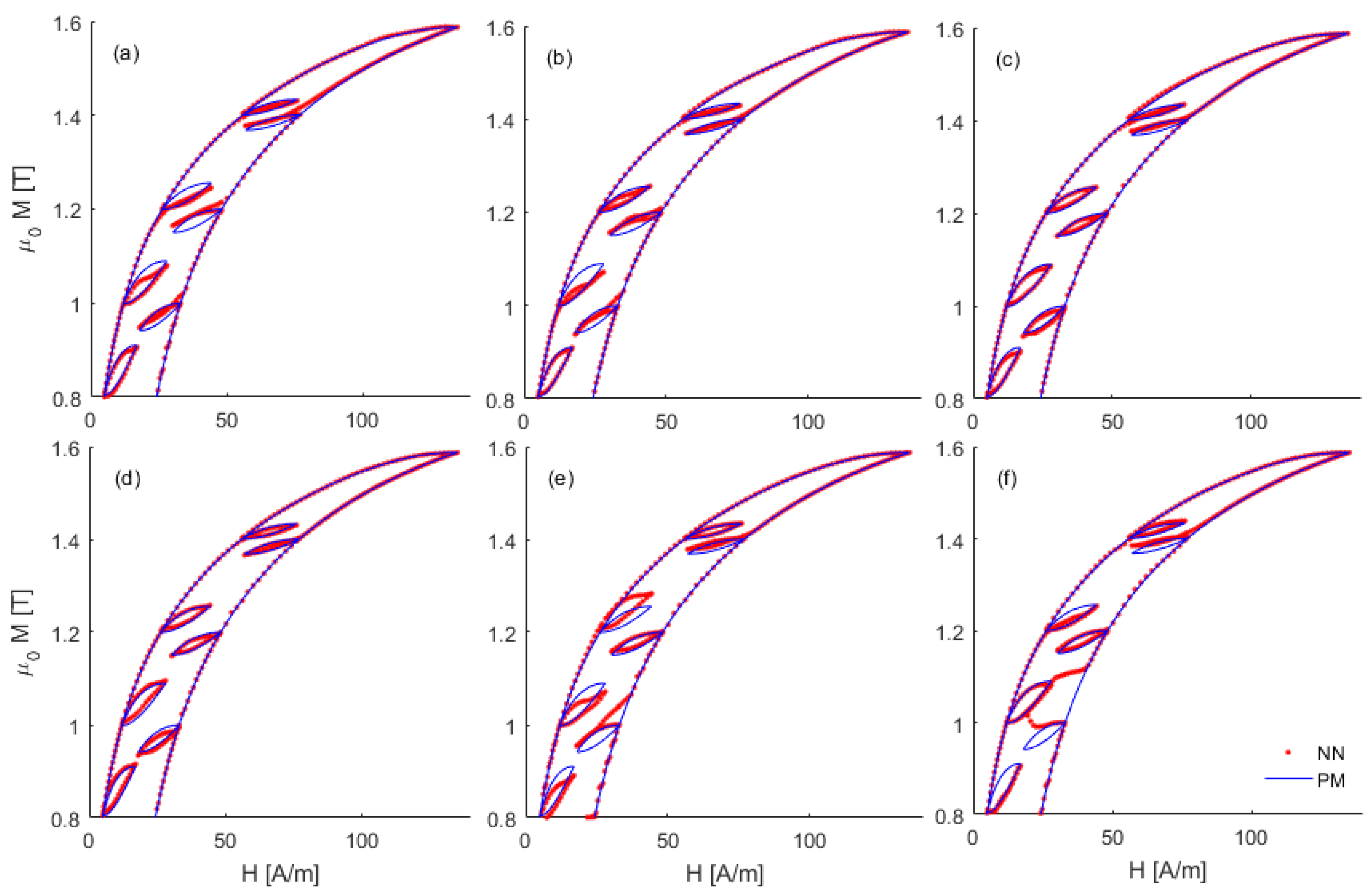
The closed-loop simulation of the training set, performed by the six trained neural networks, is illustrated in
Figure 4, where the computed loops are compared to that generated by the Preisach model. As one can note, the networks with six and eight neurons per layer, shown r in
Figure 4a,b, respectively, were undertrained; the minor loops were not always well reproduced, but the propagation of the error did not lead to numerical instability. If the number of neurons per each layer increased to 12, the reduction in training error led to a higher accuracy, as already mentioned. However, if the networks were larger, the overtraining limit was reached, as can be viewed in
Figure 4f. The largest network examined had 68 neurons (64 hidden + 3 input + 1 output) and it turned out to have too many degrees of freedom to accurately generalize the input pattern applied. The error propagation led to the closed-loop calculation of the training set being completely inaccurate.
In the present analysis, the neural network modeling was applied to grain-oriented steel. However, we are confident that the proposed method can also be suitable to simulate other soft ferromagnetic materials. In particular, non-grain-oriented (NGO) laminated alloys, showing smoother and wider hysteresis loops, as well as smaller values of the permeability and the coercive field, with respect to the grain-oriented alloys, would be easier to simulate via phenomenological hysteresis models. Of course, the whole identification must be repeated using different datasets, but we believe that the settings of the training procedure could remain unchanged.
3.3. Simulation of Symmetric Loops
The neural network with 12 neurons per hidden layer and a total number of 52 neurons turned out to be accurately trained on the dataset we generated by the PM, as well as suitable to simulate hysteresis loops with harmonics. However, we decided to firstly examine the capability of the NN-based model to reproduce quasi-static symmetric hysteresis loops under sinusoidal magnetic inductions with different amplitudes.
There are several aspects to consider. First of all, these hysteresis processes are relevant from the experimental point of view, since they can be measured in a regime state, at a low supply frequency, on reference samples and according to standardized procedures. From the regime-state symmetric loops, it is also possible to deduce other important features of the ferromagnetic alloy, such as the first magnetization curve and the maximum magnetic permeability, which are difficult to measure directly. Furthermore, they constitute the ideal working condition of electrical machines and magnetic devices, in most practical applications.
On the other hand, a family of symmetric hysteresis loops is a reference dataset for the identification of many models of hysteresis [
24,
25].
Here, we must recall that these magnetization processes were not involved in the training of the neural network, and that they allow the comparison between the two models and the experiments.
The magnetic field sequences relative to the measured loops, obtained by the Epstein testing, were applied to the input of both the PM and the NN-based model. The initial hysteron configuration of the PM is irrelevant if more than a single period is applied, but it was convenient to start the simulations from the unmagnetized state. Then, each hysteresis loop, having a given value of Hmax, was simulated tracing the first magnetization curve from H = 0 to H = Hmax, and then applying the measured sequence, opportunely shifted to start from the maximum value. Two periods were simulated, and the second one was extracted to display the hysteresis loop. The NN simulations require a similar definition of the input field, but it was preliminarily verified that the hysteresis loop calculated in the second period was not dependent on the initial magnetization state considered. For this reason, similarly to the case of the Preisach model, the NN-based model simulations could indifferently start from either Hinit = Hmax and Binit = Bmax or from the virgin state.
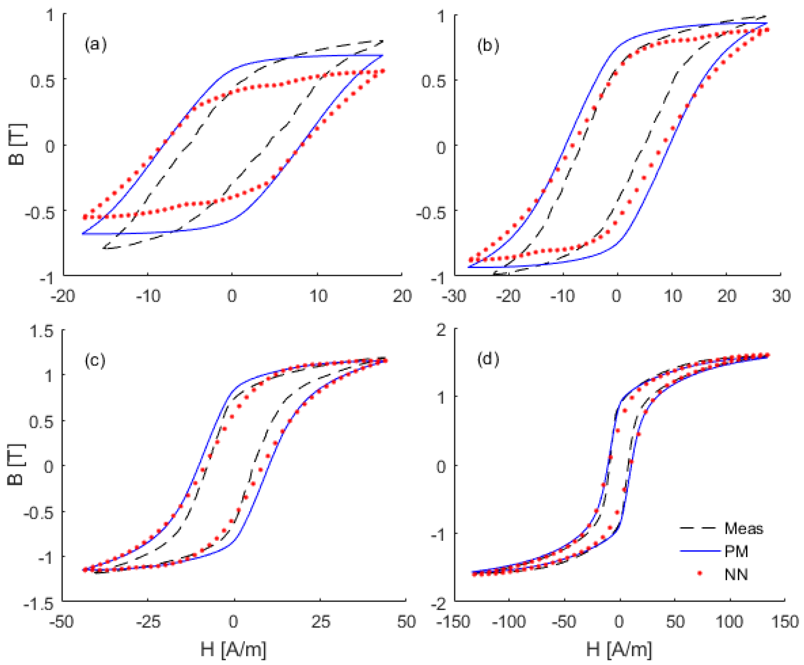
The comparison between the experimental hysteresis loops and those simulated by either the PM or the NN-based model are displayed in
Figure 5 for
Hmax = 17 A/m to
Hmax = 140 A/m. An acceptable accuracy was found in the examined range of
H. In particular, if the magnetic field was smaller than about 30 A/m, a slight deviation of the maximum value of
B simulated by the models with respect to the measured one was found. The deviations did not appear for higher values of
H, as can be seen in
Figure 5c,d.
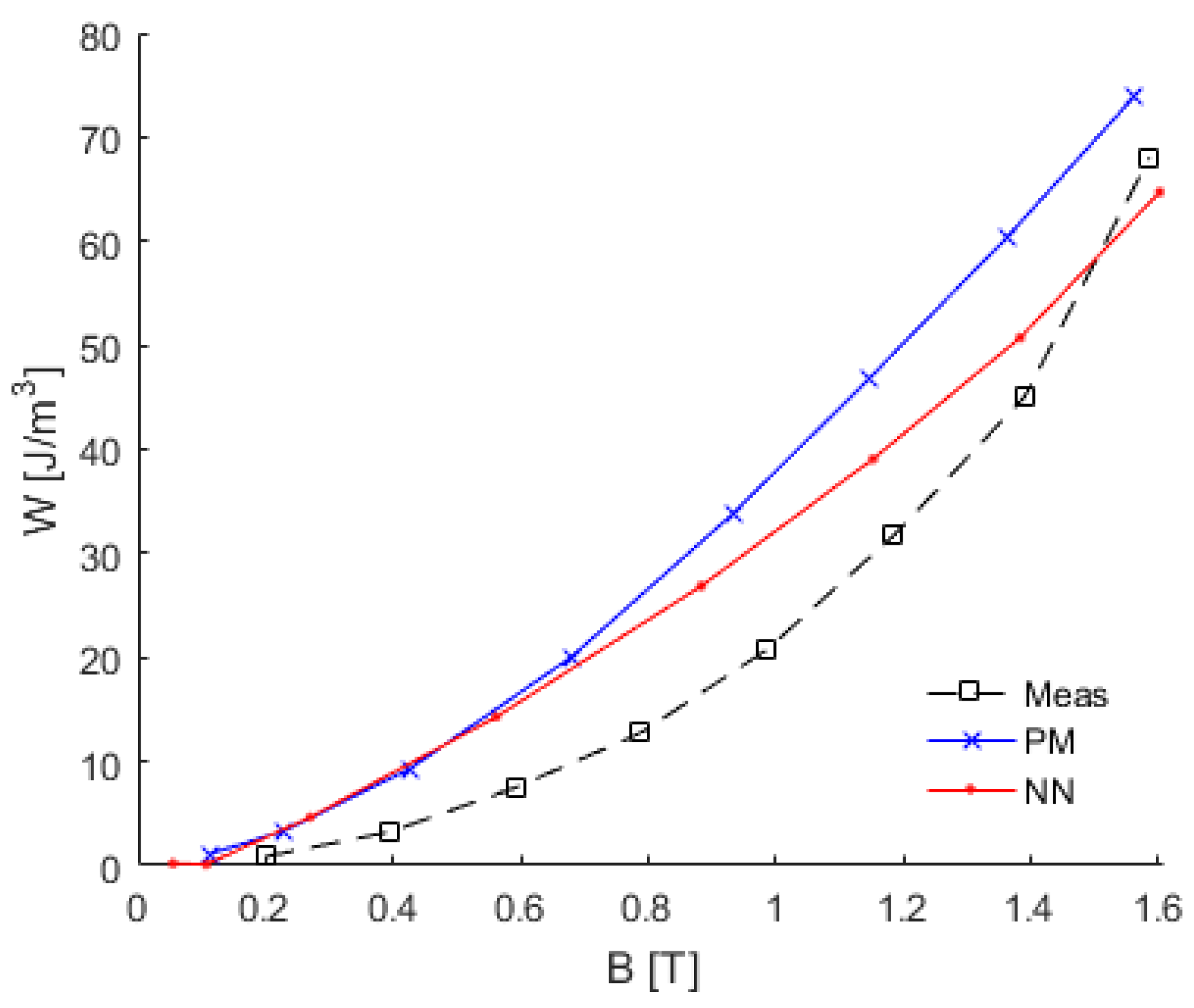
In all cases, except for the major loop, the area of the hysteresis loops simulated by both models was a bit higher with respect to that obtained by the experiments, reflecting a slight overestimation of the magnetic losses. Nevertheless, the maximum error for the estimation of the energy loss per unit of volume was found for
Bmax = 1 T, equal to 14.2 J/m
3 for the PM and 8.6 J/m
3 for the NN. The specific energy loss
W, computed from the experimental loops and those simulated by both the PM and the NN-based model, is plotted versus the maximum value of the magnetic induction in
Figure 6.
3.4. Simulation of First-Order Reversal Curves (FORCs)
The investigation then aimed to verify the capability of the NN-based model to reproduce the behavior of the PM taking into account other relevant magnetization processes, obviously not involved in the training. The NN model can, therefore, substitute the PM, thereby gaining an important saving of computational time and memory resources. The FORCs constitute an important type of hysteresis processes, from both the theoretical viewpoint, being suitable for the identification of several phenomenological models, and the application viewpoint, since they are an example of DC + AC excitation. Indeed, the cores of many electrical machines and magnetic devices for power electronics are often subjected to DC-biased magnetization loops, and the hysteresis models must be enough reliable and robust to solve them without a significant loss of precision.
We simulated a family of 16 FORCs, relative to the M4T27 material, via the PM. Each curve represents an asymmetric loop, ranging from a given minimum value (Hmin(j), Bmin(j)), with j = 1, 2, …, 16, to the same maximum value (Hmax, Bmax) = (140 A/m, 1.6 T). The coordinates of the minimum points, which represent the left corners of the asymmetric loops, were determined on the descending branch of the major loop (Bmin = −Bmax). The sequences of H and B relative to any of the 16 curves had 1000 points.
The magnetic field sequences were applied as input to the NN-based model and the computed asymmetric loops were compared to those simulated by the PM.
Figure 7 displays a comparison of some of them. The good agreement between the loop shapes obtained by the two models confirmed the capability of the NN to also replicate the Preisach simulations under more generic hysteresis patterns, quite different from those applied in the training. The differences shown in
Figure 7a,b, related to the asymmetric loops with
Hmin > 10 A/m, were almost negligible.
The specific energy losses were computed from the asymmetric loops calculated by the two hysteresis models; however, they are now plotted against the difference Δ
H(
j) =
Hmax −
Hmin(
j), for
j = 1, 2, …, 16, in
Figure 8. Since the material is almost saturated when
H =
Hmax, in the range Δ
H < 120 A/m, the asymmetric loops were quite narrow and the energy losses were lower than 10 mJ per m
3. However, for 120 A/m < Δ
H < 175 A/m, the energy losses sharply increased to about 50 mJ per m
3. For higher values of Δ
H, the loops tended to be symmetric and equal to the major cycle. In the range of Δ
H examined, the energy losses predicted by the NN-based model were very close to those obtained by the Preisach simulations.
3.5. Two-Tone Excitation Waveforms
As the conclusive step of our analysis, the hysteresis loops produced by distorted magnetic field waveforms were taken into account, with the aim of further validating the NN-based hysteresis model on a type of excitation that often occurs in magnetic cores in real applications. The presence of harmonics in the supply signal produces several unwanted effects, above all the fluctuations of the magnetic permeability and the possible formation of subloops in the main hysteresis cycle, leading to extra loss of energy.
The magnetic field sequence that we considered consisted of a fundamental component to which a third-order harmonic was added.
where
H0 = 100 A/m, and
SPP = 1000.
Once the amplitude H0 of the fundamental component and the number SPP of samples per period are fixed, two final degrees of freedom characterize the magnetic field sequence: the modulation index m and the phase displacement φ of the third harmonic with respect to the fundamental.
In order to comprehensively investigate the predictability of the NN-based model under distorted excitations, two tests were performed. In the first one, the modulation index was changed in the range [0, 0.3], covering all possible realistic values that may occur in practical working conditions. Furthermore, the phase angle between the third-order harmonic and the fundamental tone was kept constant and equal to zero. The hysteresis loops simulated by the PM indicate that, for the material examined, the subloops appeared in the main cycle if m > 0.15. In the second test, the influence of the variation of the phase angle φ on the hysteresis loops and the resulting energy losses was studied. The angle was varied between 0 and 180°, whilst the modulation index was kept constant at m = 0.24.
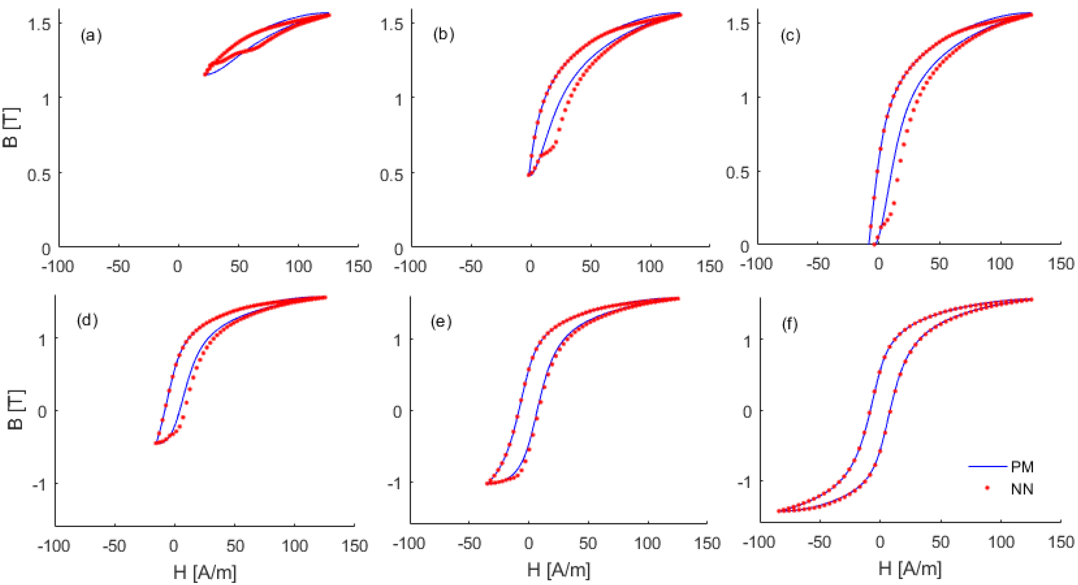
The material response under the two-tone magnetic field sequence was predicted by the PM and the NN-based model, taking into account both tests described previously. We firstly show the simulated hysteresis loops obtained for different values of
φ and
m = 0.24. The comparison between the PM- and the NN-simulated B–H curves is shown in
Figure 9.
The phase angle influenced the position of the sub-loops, which were correctly predicted by the neural network in all cases. Indeed, as can be viewed in
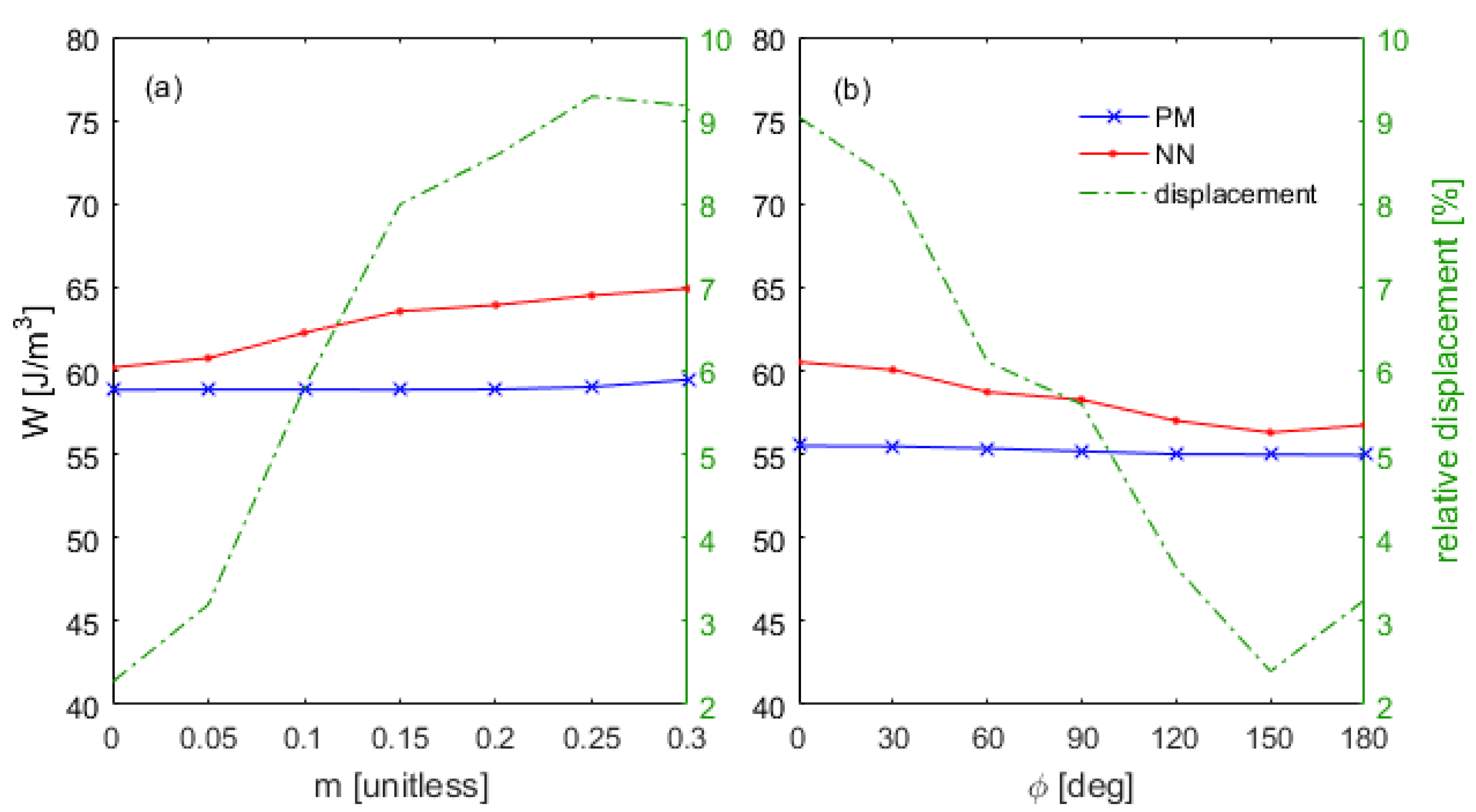
Figure 9, not only the position but also the shape of the subloops calculated by the NN were in agreement with the PM simulations. Lastly, the energy losses were estimated for both tests examined. In
Figure 10a, the specific energy loss is plotted versus the values of the modulation index, while, in
Figure 10b, it is plotted versus the angle
φ.
For M4T27 steel, according to the PM simulations, the specific energy was a weakly increasing function of m, since W passed from 58.8 J/m3 for m = 0, to 60.5 J/m3 for m = 0.3. The NN-based model tended to overestimate the losses, but the absolute error was always lower than 5 J/m3, reflecting a maximum relative displacement of 9.3%, found for m = 0.24. The displacement between the two models turned out to be an increasing function of m, as well as of the minor loop area. If the modulation index was above 0.15, the area of the minor loops became higher than the area of those present in the training set, and the increase in error was expected. However, it must be specified that such high values of the modulation index are not expected in practical applications.
The dependence of the energy loss predicted by the PM on the phase angle was very weak; W decreased from 55.5 J/m3, for φ = 0 to 54.9 J/m3, for φ = 180°. The energy losses calculated by the neural network were slightly higher than those predicted by the Preisach model, with a maximum displacement, found for φ = 0, equal to 9.1%. In this case, it is interesting to note that, for small values of the phase lag angle, the error propagation during the closed=loop calculation reflected a slight overestimation of the coercive field. This is the main reason behind the upward deviation of the energy losses computed by the NN model in the range of . For higher values of the angle, the percentage deviation was lower than 5%.
Let us conclusively give a few comments concerning the computational efficiency and the memory allocation of the models. All the simulations shown in this paper were performed on the same computer, equipped with a CPU Intel
® Core™ i7-2670 QM @ 2.20 GHz, 8 GB of RAM memory, and 64-bit operating system. The calculation speed, expressed in terms of the number of samples processed per second, was evaluated for the PM, the NN model at a high level of abstraction, and the NN at a low level of abstraction. The latter case, with 4638 samples processed per second, turned out to be the fastest approach. However, it was found out that the high-level implementation of the NN, exploiting the Neural Network Toolbox of Matlab
®, was slower than the low-level implementation of the Preisach model. The sample rate found for the neural network model at the high level of abstraction was 106 samples/s, against the 120 samples/s of the PM. It can be concluded that, in order to exploit the numerical effectiveness of the neural network, a suitable low-level implementation is necessary. The RAM memory occupied by the PM is 5.76 × 10
5 floating variables, to store the location (
Hi) and the intrinsic coercivity (
u) of all the hysterons plus 2.88 × 10
5 integer variables, to store their status at each sample step. It has to be also mentioned that some techniques have been developed recently [
26] to reduce the memory occupation of the PM. On the other hand, the RAM memory required for the NN, implemented at the low level of abstraction, only consists of 529 floating variables: 480 for the synaptic weights and 49 for the neuron bias values.
4. Conclusions
A performing numerical model of hysteresis was presented and exploited to simulate the magnetization processes of a sample of commercial grain-oriented electrical steel sheet. The core of the model is a standalone multi-layer feedforward neural network, in which the dependence on the past history is reproduced. Then, the network, unlike most approaches already proposed in the literature, does not need to be coupled with other memory-dependent models or algorithms.
In order to train the net from a minimal set of experimental loops, the Preisach model, opportunely identified for the material examined, was used to generate the training set. In addition, an optimized training procedure was defined and implemented in a graphical user interface. The optimal network architecture was individuated, as well as the undertraining and the overtraining limits. After that, the model was implemented at a low level of abstraction to improve the computational efficiency and optimize the memory allocation.
The proposed hysteresis model was validated by the reproduction of the magnetization processes in a wide range of excitations (up to 1.6 T) either obtained by the experiments or generated via the Preisach model, taking into account various types of excitation waveforms. The comparative analysis highlighted the capability of the neural network model to predict both the evolution of the material magnetization and the energy loss with a satisfactory degree of accuracy in all the examples illustrated. The computational and the memory efficiency, as well as the possibility to be easily inverted, make the model suitable for coupling with finite-element schemes.


