Wavelet-Based Three-Dimensional Inversion for Geomagnetic Depth Sounding

Abstract

The complexity of Earth’s structure poses a challenge to the multiscale detection capability of geophysics. In this paper, we present a new wavelet-based three-dimensional inversion method for geomagnetic depth sounding. This method is based on wavelet functions to transfer model parameters in the space domain into the wavelet domain. The model is represented by wavelet coefficients containing both large- and fine-scale information, enabling wavelet-based inversion to describe multiscale anomalies. L₁-norm measurement is applied to measure the model roughness to accomplish the sparsity constraint in the wavelet domain. Meanwhile, a staggered-grid finite difference method in a spherical coordinate system is used to calculate the forward responses, and the limited-memory quasi-Newton method is applied to seek the solution of the inversion objective function. Inversion tests of synthetic data for multiscale models show that wavelet-based inversion is stable and has multiresolution. Although higher-order wavelets can lead to finer results, our tests present that a db6 wavelet is suitable for geomagnetic depth sounding inversion. The db6 inversion results of responses at 129 geomagnetic observatories around the world reveal a higher-resolution image of the mantle.

1. Introduction

Geomagnetic depth sounding (GDS) is a specific electromagnetic (EM) induction technique used to detect electrical structures at depths of 200–1600 km, especially at 400–900 km [1,2,3,4,5]. Because electrical conductivity is relatively sensitive to temperature, partial melting, and the water content of minerals, GDS can reveal the subducting slabs, melting layers, mantle plumes and water transport mechanisms in deep Earth. For example, a thin melting layer located in the mid-mantle transition zone (MTZ) beneath Australia was observed through the GDS inversion of geomagnetic observatory data [6]. Evidence from electrical images for the Bermuda plume has been presented by inverting geomagnetic observatory data in North America by using GDS [7]. The electrical conductivity in the MTZ beneath Eastern China obtained by GDS suggested that water was released from the stagnant Pacific slab, wetting the MTZ, and that water may have migrated into the upper mantle and could be the source of Cenozoic interpolate volcanoes in Northeast China [8,9].

Due to the sparse and uneven distribution of geomagnetic observatories around the world, the one-dimensional (1D) inversion of GDS is suitable to detect the electrical structure beneath the observatory [4,8,10]. However, for regions with relatively dense observatories, three-dimensional (3D) inversion is the best choice to integrate the observed data from the region and obtain a more reliable result. During the three-dimensional (3D) inversions of GDS, a smoothing strategy is commonly used to balance the variations in conductivities for adjacent grid cells [1,2,7]. This strategy is suitable for revealing the gradual change in the conductivity of the Earth, such as the wet and cold MTZ caused by subducting slabs. However, for mantle plumes, melting layers and the mineral phase transition at 410 and 670 km, conductivity may jump on a local scale. Although we can set smoothing coefficients to zero to fulfill the jumping conductivity, distinguishing where the zero should be assigned is difficult.

Instead of parameterizing the Earth by using the conductivity in each grid cell, wavelet functions can transfer model parameters in the space domain into the wavelet domain, where the Earth is represented by coefficients independent of the smoothing strategy. Two types of coefficients corresponding to large- and fine-scale information of the model are used in the wavelet domain, which means that wavelet-based inversion has inherent multiresolution [11]. For the large-scale part of the model, few wavelet coefficients are sufficient; for the part with small-scale features, more coefficients must be arranged [11]. In previous studies, Chiao and Kuo [12] and Chiao and Liang [13] proposed the wavelet function for 3D seismic tomography inversion, and they used wavelet coefficients as model constraints instead of smoothness regularization in nonlinear inversion. Their simple examples show that for uneven data distributions, model variations at various scales can be robustly resolved by using the scale hierarchy in the wavelet domain depending on the distribution of the data site, and there is thus no need to invoke additional smoothness regularization. Liu et al. [11] developed a wavelet-based 3D inversion method for frequency-domain airborne EM data. Inversion results of synthetic data showed that higher-order wavelets with larger vanishing moments and regularity can deliver a more stable inversion process and give better local resolution, whereas the lower-order wavelets are simpler and less smooth, and can thus recover sharp discontinuities if the model is simple.

In this paper, we introduce the wavelet function to the 3D inversion of GDS and develop a wavelet-based inversion for GDS. Experiments were conducted to test the multiscale resolution of wavelet-based inversion and the smoothing constraint compared with traditional methods in the space domain. We aim to further analyze the most appropriate order of wavelets for inversion considering large-scale structures (300–500 km vertically, thousands of kilometers horizontally) that can be distinguished by GDS [1]. The new method is derived from a general penalty function with wavelet transform, and its solution is iteratively sought by the limited-memory quasi-Newton method (L-BFGS). A conservative staggered-grid finite difference method [14] is used to solve the forward modelling problem.

2. Methods

2.1. Theory of GDS

The inducing source of GDS is the slowly changing ring currents in the magnetosphere [15]. The currents are concentric with the magnetic equator of the Earth. Thus, numerical simulation was developed on the basis of the geomagnetic spherical coordinate system. The widely used C-response of GDS was estimated from $H_r$ (the vertical component pointing downward to the Earth’s center) and $H_{\theta }$ (the colatitudinal component pointing to magnetic north) components of the magnetic field (H) on the surface. With the assumption that ring currents can be described by the spherical harmonic function $P_1^0$ [15,16,17], C-response can be calculated as follows,

$$C\left(\omega \right)=-\frac{a_0\tan \theta }{2}\frac{H_r\left(\omega \right)}{H_{\theta }\left(\omega \right)},$$

(1)

where $a_0$ is the average radius of the Earth, $\omega$ is the angular frequency, and θ represents the geomagnetic colatitude (0°–180°). The induced geomagnetic signal collected at the surface for GDS had a period of several days to more than 100 days.

Equation (1) shows that C-responses should be calculated from the magnetic field H. Assuming the positive time harmonic dependence of the form $e^{\mathrm{i}\omega t}$, H obeys

$$\nabla \times \left(\rho \nabla \times H\right)+\mathrm{i}\omega {\mu }_{0}H=0,$$

(2)

where $\rho$ is the reciprocal of the electrical conductivity $\sigma$, ${\mu }_0$ is the vacuum magnetic permeability, and $\mathrm{i}$ is the imaginary unit. Equation (2) can be solved by using the staggered-grid finite difference method in a spherical coordinate system [14]. The model parameterized for calculation included resistive air and conductive earth. The outer boundary of air is 2$a_0$ from the surface, and its resistivity is set to a moderately large finite value of 10¹⁰ Ω m. The inner boundary of Earth is the core–mantle boundary due to the superconductive core [15]. The tangential components of H at the boundaries are specified so that Equation (2) holds throughout the space domain, whereas the resultant numerical system remains acceptably well-conditioned. The location of the $P_1^0$ source is placed at a radial distance from the Earth’s surface at 10$a_0$ to ensure that the secondary magnetic field induced by conductive earth can be considered negligible. A variant of the biconjugate gradient and an iteration method are used to obtain the solution of discretized Equation (2) [7]. Divergence correction [1] is applied to make H conservative during iteration.

2.2. General Inversion Approach

GDS inversion can generally be expressed as an optimization problem,

$$\mathsf{\Phi }\left(m,\lambda \right)\underset{m}{\to }\min ,$$

(3)

where the penalty function $\mathsf{\Phi }\left(m,\lambda \right)$ is defined by

$$\mathsf{\Phi }\left(m,\lambda \right)={\mathsf{\Phi }}_d\left(m\right)+\lambda {\mathsf{\Phi }}_m\left(m\right),$$

(4)

where ${\mathsf{\Phi }}_d\left(m\right)$ and ${\mathsf{\Phi }}_m\left(m\right)$ are the data misfit and model roughness, respectively; $\lambda$ is the regularization parameter, which is used to tradeoff ${\mathsf{\Phi }}_d\left(m\right)$ and ${\mathsf{\Phi }}_m\left(m\right)$. m is the electrical conductivity vector and, in the case of 3D inversion, represents the conductivity in each prism [18].

By using the notation of the L_p-norm measurement of the objective function, Equation (4) is expressed by

$$\mathsf{\Phi }\left(m,\lambda \right)=\Vert W_d{\left(\psi \left(m\right)-d\right)\Vert }_p^p+\lambda \Vert W_m{\left(m-m_0\right)\Vert }_p^p,$$

(5)

where d is the data vector, $m_0$ is the prior model, and $\psi$ represents the forward mapping operator to calculate the responses of model m. $W_d$ is a diagonal matrix with data covariance as diagonal elements, and $W_m$ is a smoothing matrix to relate the conductivity of each grid to that of the adjacent grids in three directions (X, Y and Z directions). The correlation among adjacent cells increases as the value of the smoothing coefficients increases from 0 to 1. L_p-norm inversion can be realized by using different values of $p$.

In the traditional inversion approach, differentiating both sides of Equation (5) with respect to the space domain model parameters and neglecting the higher-order terms of the Taylor-series expansion gives the linear system of equations to be solved at each iteration as

$$\left[J^{\mathrm{T}}{W}_d^{\mathrm{T}}{R}_d{W}_{d}J+\lambda W_m^{\mathrm{T}}{R}_m{W}_m\right]\mathsf{\delta }m=J^{\mathrm{T}}{W}_d^{\mathrm{T}}{R}_d{W}_d\left[\psi \left(m\right)-d\right]+\lambda W_m^{\mathrm{T}}{R}_m{W}_m\left(m-m_0\right),$$

(6)

where

$$R_j\left(x\right)=p{\left(x^2+{\epsilon }^2\right)}^{p/2-1},\hspace{1em}j=d\hspace{1em}\mathrm{o}\mathrm{r}\hspace{1em}m,$$

(7)

where ε is a small number to ensure the solution when $x=0$, and $p$ corresponds to the L_p-norm inversion. In the smoothness-constrained inversion, an L₂-norm measurement for the complexity of the model tends to obtain a smooth model at the boundary, whereas an L₁-norm prefers a sharper edge or focused model.

2.3. Wavelet Domain Inversion

$m$ in the space domain can be transformed into coefficients ($\tilde{m}$) in the wavelet domain by using a wavelet transform matrix $W_w$:

$$\tilde{m}=W_{w}m.$$

(8)

This wavelet transform of the model can be treated as a filtering process, and the filtering coefficients are given in Daubechies [19]. Because the transform is designed in a one-dimensional (1D) setting, we propose the 3D inversion following the transform scheme of Liu et al. [11]. The transform is applied in three directions, similar to the common smoothing constraint in the space domain. The Jacobian matrix needed in the wavelet domain can be obtained by using the chain rule and expressed as

$$\tilde{J}=J{W}_w^{-1},$$

(9)

where $W_w^{-1}$ is the inverse wavelet transform operator. The matrix $W_w$ is orthonormal, and its inverse can be calculated by its transpose,

$$W_w^{-1}=W_w^{\mathrm{T}},$$

(10)

where the superscript T denotes the transpose operation. Thus, we have the following identity:

$$I=W_w^{-1}{W}_w=W_w^{\mathrm{T}}{W}_w=W_w{W}_w^{\mathrm{T}},$$

(11)

where $I$ is the identity matrix.

The linear system of Equation (6) can be expressed by

$$\left[{\tilde{J}}^{\mathrm{T}}{W}_d^{\mathrm{T}}{R}_d{W}_d\tilde{J}+\lambda R_m\right]\mathsf{\delta }\tilde{m}={\tilde{J}}^{\mathrm{T}}{W}_d^{\mathrm{T}}{R}_d{W}_d\left[\psi \left(m\right)-d\right]+\lambda R_m\left(\tilde{m}-{\tilde{m}}_0\right),$$

(12)

where the smoothing operator $W_m$ for the model is no longer needed because the constraint can be inherently generated by the wavelet-based representation.

2.4. L-BFGS Technique

The optimization of Equation (3) in the case of GDS inversion is nonlinear. Thus, we selected the L-BFGS method, which has been widely used in EM induction exploration [7,20] to minimize the penalty function. L-BFGS is a modified form of the quasi-Newton method. Its basic iteration formula is

$$m_{k+1}=m_k+{\alpha }_k{p}_k,$$

(13)

where

$$p_k=-B_k^{-1}\nabla {\mathsf{\Phi }}_k,$$

(14)

and

$$\nabla {\mathsf{\Phi }}_k={\left.{\left(\frac{\partial \mathsf{\Phi }}{\partial m_1},\frac{\partial \mathsf{\Phi }}{\partial m_2},\cdots ,\frac{\partial \mathsf{\Phi }}{\partial m_{\mathrm{N}}}\right)}^{\mathrm{T}}\right|}_{m=m_k}.$$

(15)

Here, $k$ is the number of iterations, ${\alpha }_k$ is the searching step, $p_k$ is the searching direction and $B_k$ is the approximation of the Hessian matrix [21]. The approximation of the Hessian matrix avoids its direct calculation, thus tremendously reducing the requirement for computer storage and computation time.

The computation of Equation (12) requires the calculation of the Jacobian matrix and forward responses. The latter can be easily accomplished. Nominally, the Jacobian matrix can be directly computed, but the adjoint forward technique—a more feasible method—can also be considered [1,7,22]. By using this method, we computed the product of the matrix and the data vector, which was split into a few adjacent forward operations, thus greatly reducing computational requirements.

3. Synthetic Examples

3.1. Selection of the Wavelet Order and L_p-Norm Measurement

Because the Daubechies (db) wavelet has a good regularity to guarantee a relatively smooth and actual recovery of the input model and because its basis functions are orthogonal and biorthogonal, we selected it to test the resolution and stability of the wavelet-based inversion of GDS. The selection of the wavelet order is determined by the regularity and vanishing moment. Regularity defines the smoothness of the wavelet function, whereas the vanishing moment defines the flatness and the oscillation of the wavelet function. Wavelet function can represent discontinuous signals better with a smaller-order N, and we can recover the discontinuous boundary better in the model. For a larger N, a smooth and focused model is obtained, leading the inversion to be more stable with a higher resolution [11]. However, a wavelet with a very high order may produce fake anomalies due to the strong oscillation or rapid variation basis function. Additionally, Earth should be divided into cells approximately hundreds of kilometers in size, considering the vertical and horizontal resolutions of GDS. Wavelet transform demands that the order of the matrix should be a multiple of two and the dimension of the vector should be in the power of two. Therefore, three different wavelets in the order of 2 (db2), 6 (db6) and 10 (db10) (Figure 1) were tested in this paper. We divided the conductive earth into 16 spherical layers from the surface to the core (0–2890 km), and 32 cells in longitude and 16 cells in latitude were used to parametrize the model horizontally.

The coefficients in the wavelet domain contain both large- and fine-scale information, meaning that the wavelet-based inversion has multiresolution properties [11,13,19]. By using the global average 1D conductivity model (Figure 2a) derived from vector magnetic field data observed in satellites [23], we built a model (Figure 2b) with multiscale anomalies to show how the model is present in the wavelet domain. The anomalies were assigned at depths of 670–900 km, corresponding to the most sensitive depth of GDS [1], to exclude interference factors for inversion results as much as possible. Small-scale anomalies occupied a cell, and two cells were placed at the sides of the model. Two linear anomalies were placed on the north and south sides. The other two large-scale inclining anomalies were located in the center of the model. The conductivity of the anomalies was one order around the magnitude of the background (homogeneous) model value.

The model can be transferred into the wavelet domain by using the wavelet transform matrix, and we draw the wavelet coefficients of wavelets of different orders in Figure 3. In the wavelet domain, the model is represented by two groups of coefficients: one is the group of approximate coefficients with large values, and the other comprises detailed coefficients with small values. An L₂-norm measurement of the coefficients could excessively enlarge the difference between the large and small coefficients, leading to the invisibility of detailed information. Simultaneously, considering that wavelet coefficients are sparse, a sparsity constraint is needed instead of the smoothing constraint in the space domain [24]. According to Donoho [25], the L₁-norm measurement can lead to a sparse solution. Thus, the L₁-norm measurement is chosen in our GDS inversion in the wavelet domain. For the data misfit term, L₂-norm measurement is used in our numerical tests considering the Gaussian noise added in the synthetic data. However, for actual data observed from observatories with large noises, L₁-norm measurement is suggested by Li et al. [7].

3.2. Tests for Multiresolution Based on a Regular Network

A model with multiscale anomalies was used to examine the multiresolution of the wavelet-based inversion of GDS. A data-set with 129 observatories was selected from the global observatory data sets for detecting mantle electrical conductivity [7] and the resolution of GDS; thus, we created a hypothetical regular network with 120 sites in total for the inversion tests (Figure 4). The sites were located between −56° and 56° geomagnetic latitude and started from zero geomagnetic longitude, and the latitudinal and longitudinal distances between the adjacent locations were 16° and 24°, respectively [1]. Sixteen periods of C-responses logarithmically ranged from 3 to 116 days, and synthetic data were obtained by adding 5% Gaussian random noises to the numerical modelling responses of the testing model.

Inversions in the wavelet domain with db2, db6, db10, and L₁- and L₂-norm inversions based on the traditional space domain were conducted, and we discuss here the differences between wavelet-based inversions and L_p-norm (p = 1 and 2) inversion in terms of both resolution and stability. L_p-norm inversion can be developed according to Equation (5). For L₁-norm-type inversions (L₁-norm, db2, db6 and db10 inversions), we set the value of $\epsilon$ to 10⁻⁴ and kept it constant throughout the inversion. Iterative inversion started from the 1D background model. The value of the regularization parameter ($\lambda$) started from 100 and decreased progressively when the value of the searching step was too small or the data misfit reduced very slowly. All inversions were performed with the same starting regularization parameter and updating strategy.

Slices of inversion models in the XOY plane are shown in Figure 5a–e. The results show that the principal features can be revealed by all inversions in the right layer. For L₁-norm-type inversions, the inverted model’s distribution was much more focused compared with that of L₂-norm inversion. The shape and conductivity of inclining anomalies on a large-scale can be described well in all inversions, but the stair–step shape was more obvious in the L_p-norm inversion with a slightly expanded boundary. Compared with db6 and db10, db2 was not suitable for presenting complex structures and led to the disharmonic imaging of anomalies because the wavelet function and the model freedom were relatively simple (Figure 1a). For linear anomalies, wavelet-based inversions had much better resolutions than that of the L_p-norm inversion, especially in the latitudinal direction, where an obviously expanded boundary was obtained in L_p-norm inversions. The recovered linear anomaly with enhanced conductivity was more like a blocky anomaly than a banded anomaly in the L_p-norm inversions, especially in the L₂-norm inversion. Small-scale anomalies could be recovered well by all L₁-norm type inversions but were more difficult to recognize with L₂-norm inversion, which we attribute to the oversmoothing between adjacent cells caused by the smoothing strategy of the L₂-norm measurement. In all inversions, the amplitude of the conductivity, especially the resistive one, was inadequately obtained. This was caused by the leakage of conductance to adjacent layers, which is inevitable in geophysical inversion [1]. Although the leakage occurred in all inversions, Figure 5 illustrates that db10 was in very high order for GDS inversion, possibly related to the relatively rough resolution of GDS, whereas db2 and db6 could suppress the leakage to some extent.

Variations in inversion parameters with iterations are shown in Figure 6. All inversions were terminated with a root mean square (RMS) of data misfit close to 1.0. This means that the responses of the inverted model fit the synthetic data well, and that the wavelet-based inversion was effective. The curves changed gently near the termination, indicating that the processes of the wavelet-based inversions were stable. Compared with L₂-norm inversion, the RMS of L₁-norm inversion decreased more slowly. This may be attributed to the relatively small model roughness at the beginning, as the small value of ε makes ${\mathsf{\Phi }}_m$ much larger than that measured by the L₂-norm according to Equation (7) and lowers the weight of data misfit in the penalty function. This situation was solved in wavelet-based inversions, indicating they can balance the weight of data misfit and model roughness. Thus, we can speculate that wavelet-based inversions are less influenced by the starting regularization parameter. The model roughness of the inversions based on the L₁-norm measurement was larger than that of the L₂-norm inversion (Figure 6c) because the enlargement of squared estimation prefers a smoothing model and suppresses the amplitude of anomaly. This means sharper boundaries are preferred in inversions based on the L₁-norm-type measurement.

The conductivity of adjacent layers can be allowed to jump in the L_p-norm inversions if we set the smooth coefficients to zero. Thus, we conducted these inversions and compared the results with wavelet-based inversion, in which the conductivities are allowed to jump at the upper (670 km) and lower (900 km) boundaries of the layer (670–900 km) with anomalies. Figure 7 shows that the results of L_p-norm inversions are more concentrated in the right layer with anomalies than those without jump constraint (Figure 6a,b). Vertically, the wavelet-based inversion shares a similar capacity for reconstructing the anomaly with L_p-norm inversion in which the conductivities are allowed to jump. However, the reconstruction of multiscale anomalies is still a challenge for L_p-norm inversions. We contribute this deficiency to the smoothing strategy in the horizontal plane. Although the leakage of conductance cannot be resolved by the wavelet-based inversion, it provides an efficient method to obtain a reliable model instead of the trying and choosing in L_p-norm inversions.

Overall, the smoothing constraint in the space domain is suitable for large-scale anomalies but is not beneficial in describing small-scale and banded anomalies. An important reason is that the conductivity of a cell is apportioned to adjacent cells by the smoothing constraint; thus, the inversion prefers to obtain a smoothing model instead of a focusing one, where obtaining a clear boundary is hard. Through numerical tests, we verified the multiresolution of wavelet-based inversion, and db6 inversion was suitable for GDS inversion.

3.3. More Realistic Tests Based on the Distribution of Real Observatories

A data set with 129 observatories (Figure 8) located in low- and mid-latitudes were selected from global observatory data sets (World Data Centre, http://www.wdc.bgs.ac.uk, accessed on 30 June 2022) [7] to invert the mantle electrical structure by using GDS. Given the number of sites used in the inversion, the data set can provide a more reliable model and better constraints on the shape and range of anomalies [7]. We tested the resolution of wavelet-based inversion (db6) depending on the distribution of 129 observatories, compared with that in the L_p-norm inversion. Synthetic data were obtained by adding 5% Gaussian noise to the forward responses, and the background model, initial regularization parameter, and other parameters for inversion were the same as those in the former tests.

A checkerboard model with equally distributed anomalies across the spherical layer was used in our tests. The forward model was determined according to the spherical harmonic function ${\rho }_k\left(\theta ,\phi \right)$ in a general form

$$\log {\rho }_k\left(\theta ,\phi \right)=a_0^0+{\sum }_{l=1}^L\left[a_l^0{P}_l\left(\cos \theta \right)+\left[{\sum }_{m=1}^l\begin{array}{c}{a}_l^m\cos \left(m\phi \right)+\\ {\sum }_{m=-1}^{-l}{a}_l^m\sin \left(m\phi \right)\end{array}\right]S_l^m\left(\cos \theta \right)\right],$$

(16)

where θ and ϕ are the latitude and longitude in the geomagnetic coordinates, respectively; $S_l^m$ represents the Schmidt semi-normalized associated Legendre functions; l and m are the degree and order of the spherical harmonic, respectively, $P_l$ is a special case of $S_l^m$ when m = 0, L is the largest degree, and $a_l^m$ is the coefficient of the spherical harmonic with degree l and order m. We set the coefficient $a_{12}^6$ to 2.3 to create a checkerboard model with an average anomaly size of about 20° × 20° (as shown in Figure 8), corresponding to the thousands of kilometers of the horizontal resolution of GDS [1], and to restrict conductivity variations within the layer to one order around the magnitude of the background model value.

The inversion results (Figure 9) of the checkerboard model show that db6 and L_p-norm inversion can reveal the position and shape of the checkerboard model in regions where there are sufficient observatories. Thus, the resolution of GDS is much higher in the northern hemisphere than in the southern hemisphere, which can be attributed to the denser geomagnetic observatories distributed in the northern hemisphere. Moreover, the recovered anomalies were focused on the right layer. However, because the distribution of observatories is, nowadays, spatially irregular and sparse, identifying anomalies in areas with little coverage from observatories is not feasible. Compared with L_p-norm inversion, db6 inversion can obtain more details on these anomalies, and the conductivities are much closer to the actual values, especially for resistive anomalies. The shape of the checkerboard was perturbed or connected with the neighbor anomaly in L_p-norm inversion, and a mass of conductance or resistance was leaked to the shallower and deeper layers. The situation further demonstrates that the smoothing constraint in the space domain influences the reliability of inversion results and may derive dramatically different results. This challenge was solved perfectly by wavelet-based inversion because the smoothing constraint was contained in the wavelet transform.

4. Inversion of Actual Data

Geomagnetic field data have been widely used to detect the inner structure of the Earth [26,27]. Synthetic examples show that a multiscale and reliable result can be derived from db6 GDS inversion. Thus, we inverted the C-responses estimated by the geomagnetic field recorded by the 129 stations selected in our previous work [7]. C-responses at stations are estimated by processing the geomagnetic filed with a self-referenced BIRRP method [7,28]. The obtained C-responses are shown in Figure 10. As a quality indicator, squared coherency with a large value is treated as a response with good quality [7]. Thus, Figure 10b indicates that C-responses in some stations have poor quality. Considering that large data noise would cause deformation and even fake anomalies [29,30], the L₁-norm-type measuring data misfit term was used to suppress the influence of large noise [7,31,32]. The initial model of inversion adopted the 1D model in Figure 2. Earth was divided into 16 layers vertically and 32 × 16 grid horizontally, as undertaken in the synthetic tests. A lateral grid of 1° × 1° within 12.65 km of the surface layer containing ocean and land was considered in the forward modelling to eliminate the ocean effect [3,33,34]. The conductance of the surface layer was obtained from Everett et al. [35]. The conductivity of the surface layer was frozen in the inversion and was not transformed into the wavelet domain. The initial regularization parameter and its decreasing strategy were the same as those in the synthetic data inversions. The inversion terminated after 91 iterations with an RMS misfit to the observed data of 2.4, significantly larger than the expected value of 1.0. This large RMS is due to some unreliable data included in the inversion [7]. The data fitting curves in some stations are shown in Figure 11. The curves show a good fitting for the majority of responses, indicating the convincing results of our inversion.

Figure 12a displays the inverted electrical structure of the wavelet-based inversion of GDS in the MTZ and the lower mantle. The main electrical variations were concentrated in the depth range between 410 and 900 km, corresponding to the most sensitive zone of GDS. Meanwhile, the 3D model shares the main features revealed by Li et al. (Figure 12b) [7]; for instance, the conductivities increase beneath East Asia but decrease beneath southern Europe and northern Africa, and a conductive region emerges underneath south Australia. Because of the multiresolution of the wavelet-based inversion, the db6 inversion result differed from that of the traditional L_p-norm inversion and gave rise to more convincing features in the model. The resistive anomalies behaved more obviously, and the boundary was much clearer. In lower MTZ, an isolated enhanced conductivity anomaly was present instead, connecting with the Bermuda anomaly [7]. The conductivity zone in east China was more concentrated in northeast China, which could be related to the released water from the stagnant Pacific slab [8]. Between South America and Antarctica, conductive anomalies were more localized in the topmost lower mantle and more continuous in the lower mantle. A conductive area near the Philippine Sea was present in the wavelet-based inversion instead of the resistive zone. However, we cannot confirm the stability of this anomaly because of the lack of data coverage. In deeper mantle (>900 km), the recovered anomaly of L_p-norm inversion was smoother both vertically and horizontally, whereas more localized anomalies were revealed by the wavelet-based inversion.

5. Conclusions

In this paper, we presented a sparse constraint 3D inversion for GDS based on the wavelet function. The conductive earth was parameterized, and inversion was performed in the wavelet domain instead of the space domain. The L₁-norm measurement was used to measure the model roughness, whereas the data misfit was still measured by using the L₂-norm in wavelet-based inversion. The new algorithm was applied to invert synthetic data and field C-responses estimated in our previous work. The following conclusions can be drawn from these inversion results:

(1)

The db6 inversion is suitable for GDS inversion, and orders that are too high are not suitable, which may be related to the resolution of GDS;

(2)

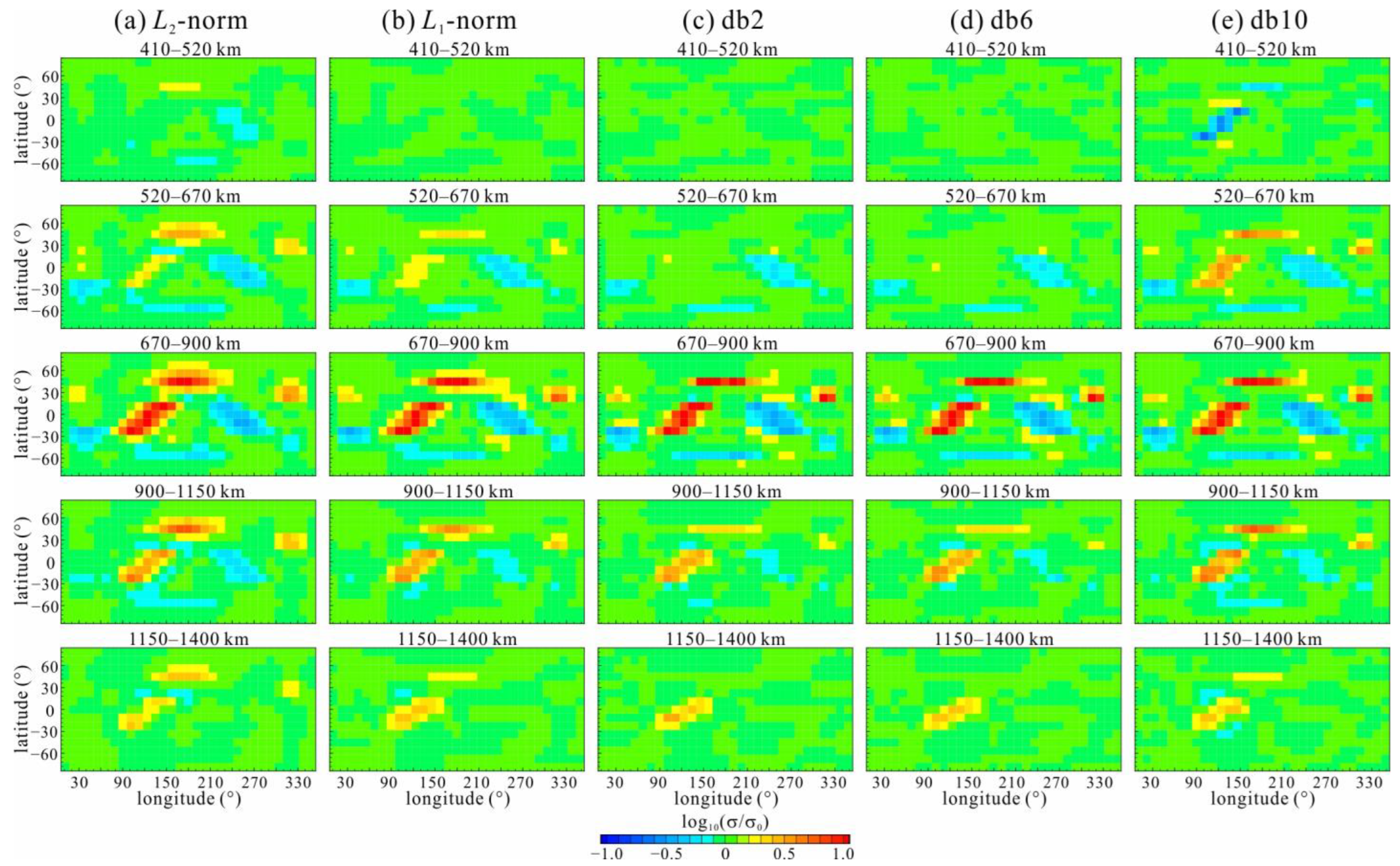
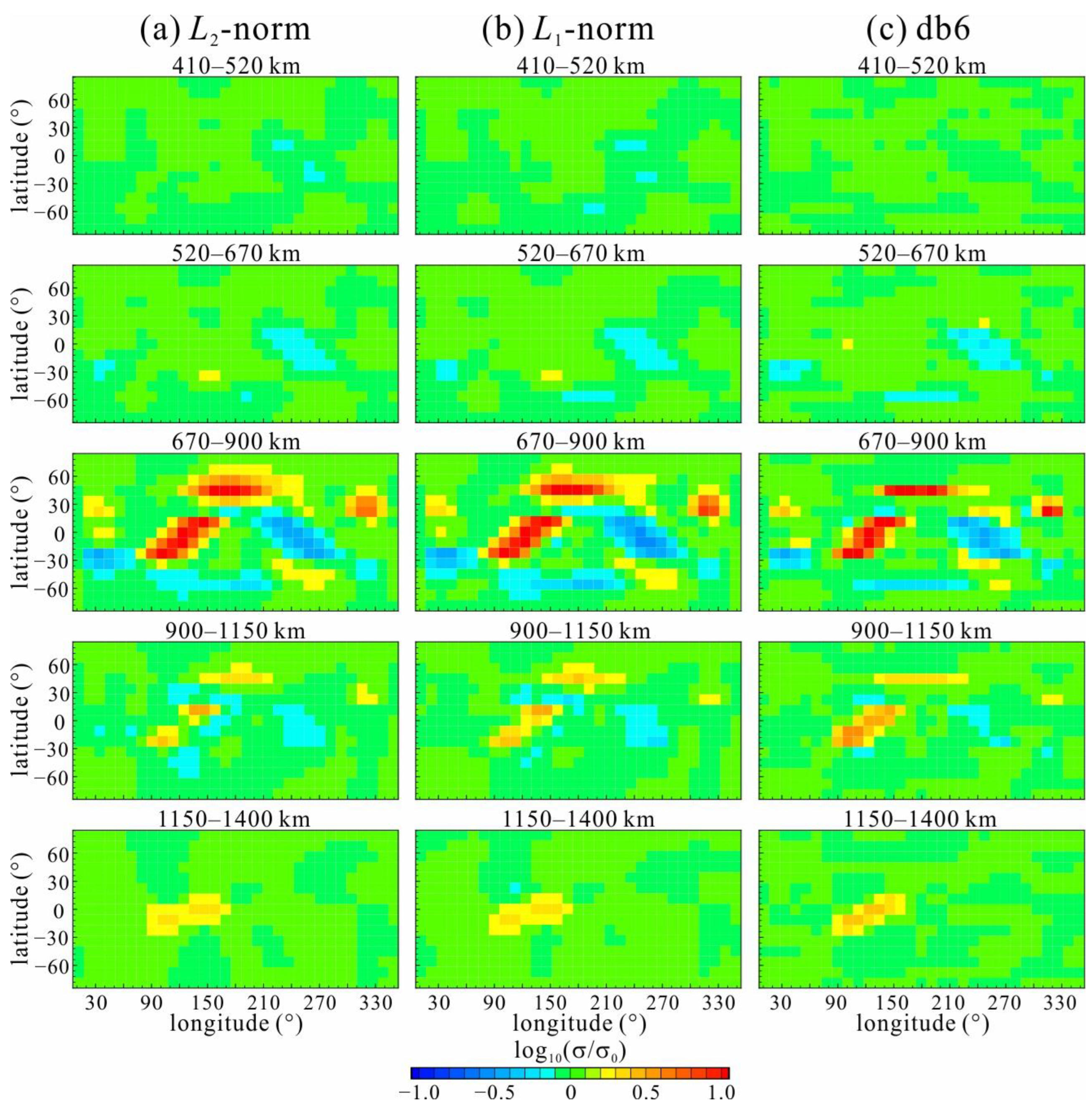
The db6 inversion has a better resolution than the L_p-norm inversion for a model with multiscale anomalies, especially for small-scale and linear anomalies;

(3)

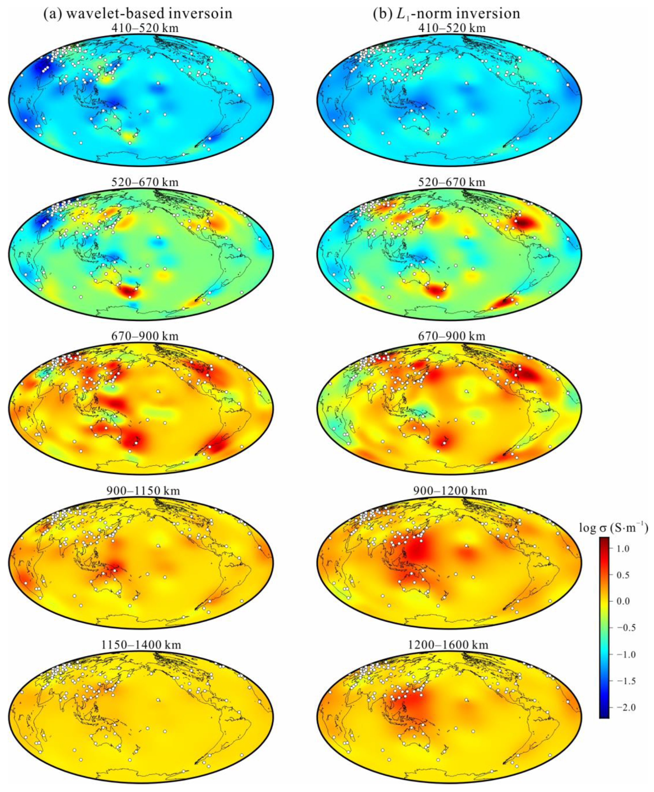
The inversion of global C-responses for 129 observatories presents features similar to those of previously published anomalies, but a much higher-resolution image of the mantle is given by db6 inversion.

References

1. Kelbert, A.; Egbert, G.D.; Schultz, A. Non-Linear Conjugate Gradient Inversion for Global EM Induction: Resolution Studies. Geophys. J. Int. 2008, 173, 365–381. [Google Scholar] [CrossRef]
2. Kelbert, A.; Schultz, A.; Egbert, G. Global Electromagnetic Induction Constraints on Transition-Zone Water Content Variations. Nature 2009, 460, 1003–1006. [Google Scholar] [CrossRef] [PubMed]
3. Semenov, A.; Kuvshinov, A. Global 3-D Imaging of Mantle Conductivity Based on Inversion of Observatory C-Responses-II. Data Analysis and Results. Geophys. J. Int. 2012, 191, 965–992. [Google Scholar] [CrossRef] [Green Version]
4. Yuan, Y.; Uyeshima, M.; Huang, Q.; Tang, J.; Li, Q.; Teng, Y. Continental-Scale Deep Electrical Resistivity Structure Beneath China. Tectonophysics 2020, 790, 228559. [Google Scholar] [CrossRef]
5. Püthe, C.; Kuvshinov, A.; Khan, A.; Olsen, N. A New Model of Earth’s Radial Conductivity Structure Derived from over 10 Yr of Satellite and Observatory Magnetic Data. Geophys. J. Int. 2015, 203, 1864–1872. [Google Scholar] [CrossRef] [Green Version]
6. Koyama, T.; Khan, A.; Kuvshinov, A. Three-Dimensional Electrical Conductivity Structure beneath Australia from Inversion of Geomagnetic Observatory Data: Evidence for Lateral Variations in Transition-Zone Temperature, Water Content and Melt. Geophys. J. Int. 2014, 196, 1330–1350. [Google Scholar] [CrossRef] [Green Version]
7. Li, S.; Weng, A.; Zhang, Y.; Schultz, A.; Li, Y.; Tang, Y.; Zou, Z.; Zhou, Z. Evidence of Bermuda Hot and Wet Upwelling from Novel Three-Dimensional Global Mantle Electrical Conductivity Image. Geochem. Geophys. Geosystems 2020, 21, e2020GC009016. [Google Scholar] [CrossRef]
8. Zhang, Y.; Weng, A.; Li, S.; Yang, Y.; Tang, Y.; Liu, Y. Electrical Conductivity in the Mantle Transition Zone beneath Eastern China Derived from L1-Norm C-Responses. Geophys. J. Int. 2020, 221, 1110–1124. [Google Scholar] [CrossRef]
9. Li, S.; Weng, A.; Li, J.; Shan, X.; Han, J.; Tang, Y.; Zhang, Y.; Wang, X. Deep Origin of Cenozoic Volcanoes in Northeast China Revealed by 3-D Electrical Structure. Sci. China Earth Sci. 2020, 63, 533–547. [Google Scholar] [CrossRef]
10. Guo, J.; Lian, X.; Wang, X. Electrical Conductivity Evidence for the Existence of a Mantle Plume beneath Tarim Basin. Appl. Sci. 2021, 11, 893. [Google Scholar] [CrossRef]
11. Liu, Y.; Farquharson, C.G.; Yin, C.; Baranwal, V.C. Wavelet-Based 3-D Inversion for Frequency-Domain Airborne EM Data. Geophys. J. Int. 2018, 213, 1–15. [Google Scholar] [CrossRef]
12. Chiao, L.-Y.; Kuo, B.-Y. Multiscale Seismic Tomography. Multiscale Seism. Tomogr. 2001, 145, 517–527. [Google Scholar] [CrossRef]
13. Chiao, L.-Y.; Liang, W.-T. Multiresolution Parameterization for Geophysical Inverse Problems. Geophysics 2003, 68, 199–209. [Google Scholar] [CrossRef]
14. Uyeshima, M.; Schultz, A. Geoelectromagnetic Induction in a Heterogeneous Sphere: A New Three-Dimensional Forward Solver Using a Conservative Staggered-Grid Finite Difference Method. Geophys. J. Int. 2000, 140, 636–650. [Google Scholar] [CrossRef] [Green Version]
15. Banks, R.J. Geomagnetic Variations and the Electrical Conductivity of the Upper Mantle. Geophys. J. R. Astron. Soc. 1969, 17, 457–487. [Google Scholar] [CrossRef] [Green Version]
16. Grayver, A.V.; Munch, F.D.; Kuvshinov, A.V.; Khan, A.; Sabaka, T.J.; Tøffner-Clausen, L. Joint Inversion of Satellite-Detected Tidal and Magnetospheric Signals Constrains Electrical Conductivity and Water Content of the Upper Mantle and Transition Zone. Geophys. Res. Lett. 2017, 44, 6074–6081. [Google Scholar] [CrossRef] [Green Version]
17. Munch, F.D.; Grayver, A.V.; Kuvshinov, A.; Khan, A. Stochastic Inversion of Geomagnetic Observatory Data Including Rigorous Treatment of the Ocean Induction Effect with Implications for Transition Zone Water Content and Thermal Structure. J. Geophys. Res. Solid Earth 2018, 123, 31–51. [Google Scholar] [CrossRef]
18. Zhao, D. Global Tomographic Images of Mantle Plumes and Subducting Slabs: Insight into Deep Earth Dynamics. Phys. Earth Planet. Inter. 2004, 146, 3–34. [Google Scholar] [CrossRef]
19. Daubechies, I. Ten Lectures on Wavelets; Society for Industrial and Applied Mathematics: Philadelphia, PA, USA, 1992; ISBN 9781611973280. [Google Scholar]
20. Avdeev, D.; Avdeeva, A. 3D Magnetotelluric Inversion Using a Limited-Memory Quasi-Newton Optimization. Geophysics 2009, 74, F45–F57. [Google Scholar] [CrossRef] [Green Version]
21. Nocedal, J.; Wright, S.J. Numerical Optimization, 2nd ed.; Thomas, V., Resnick, M., Robinson, S.M., Eds.; Springer Science + Business Media, LLC: New York, NY, USA, 2006; Volume 17, ISBN 0196-0202. [Google Scholar]
22. Egbert, G.D.; Kelbert, A. Computational Recipes for Electromagnetic Inverse Problems. Geophys. J. Int. 2012, 189, 251–267. [Google Scholar] [CrossRef]
23. Kuvshinov, A.; Olsen, N. A Global Model of Mantle Conductivity Derived from 5 Years of CHAMP, Ørsted, and SAC-C Magnetic Data.Pdf. Geophys. Res. Lett. 2006, 33, 1–5. [Google Scholar] [CrossRef]
24. Daubechies, I.; Defrise, M.; De Mol, C. An Iterative Thresholding Algorithm for Linear Inverse Problems with a Sparsity Constraint. Commun. Pure Appl. Math. 2004, 57, 1413–1457. [Google Scholar] [CrossRef] [Green Version]
25. Donoho, D.L. For Most Large Underdetermined Systems of Linear Equations the Minimal L1-Norm Solution Is Also the Sparsest Solution. Commun. Pure Appl. Math. 2006, 59, 797–829. [Google Scholar] [CrossRef]
26. Zahedi, R.; Daneshgar, S.; Ali, M.; Seraji, N.; Asemi, H. Modeling and Interpretation of Geomagnetic Data Related to Geothermal Sources, Northwest of Delijan. Renew. Energy 2022, 196, 444–450. [Google Scholar] [CrossRef]
27. Zahedi, R.; Babaee, A. Numerical and Experimental Simulation of Gas-Liquid Two-Phase Flow in 90-Degree Elbow. Alex. Eng. J. 2022, 61, 2536–2550. [Google Scholar] [CrossRef]
28. Chave, A.D.; Thomson, D.J. Bounded Influence Magnetotelluric Response Function Estimation. Geophys. J. Int. 2004, 157, 988–1006. [Google Scholar] [CrossRef]
29. Li, G.; Liu, X.; Tang, J.; Deng, J.; Hu, S.; Zhou, C.; Chen, C. Improved Shift—Invariant Sparse Coding for Noise Attenuation of Magnetotelluric Data. Earth Planets Sp. 2020, 72, 1–15. [Google Scholar] [CrossRef] [Green Version]
30. Li, G.; Liu, X.; Tang, J.; Li, J.; Ren, Z.; Chen, C. De-Noising Low-Frequency Magnetotelluric Data Using Mathematical Morphology Fi Ltering and Sparse Representation. J. Appl. Geophys. 2020, 172, 103919. [Google Scholar] [CrossRef]
31. Farquharson, C.G. Constructing Piecewise-Constant Models in Multidimensional Minimum-Structure Inversions. Geophysics 2008, 73, K1–K9. [Google Scholar] [CrossRef]
32. Menke, W. Geophysical Data Analysis: Discrete Inverse Theory; Academi C Press, Inc.: Orlando, FL, USA, 1984. [Google Scholar]
33. Chen, C.; Kruglyakov, M.; Kuvshinov, A. A New Method for Accurate and Efficient Modeling of the Local Ocean Induction Effects. Application to Long-Period Responses from Island Geomagnetic Observatories. Geophys. Res. Lett. 2020, 47, 1–9. [Google Scholar] [CrossRef]
34. Yao, H.; Ren, Z.; Tang, J.; Zhang, K. A Multi-Resolution Finite-Element Approach for Global Electromagnetic Induction Modeling with Application to Southeast China Coastal Geomagnetic Observatory Studies. J. Geophys. Res. Solid Earth 2022, 127, e2022JB024659. [Google Scholar] [CrossRef]
35. Everett, M.E.; Constable, S.; Constable, C.G. Effects of Near-Surface Conductance on Global Satellite Induction Responses. Geophys. J. Int. 2003, 153, 277–286. [Google Scholar] [CrossRef]
Figure 1. Scaling functions of the wavelet with varying orders (db2, db6 and db10). (a) db2, (b) db6, (c) db10.
Magnetochemistry 08 00187 g001
Figure 2. Global average one-dimensional (1D) conductivity model (a) and the model with multiscale anomalies at depths of 670–900 km (b).
Magnetochemistry 08 00187 g002
Figure 3. Wavelet coefficients of the forward model in the space domain (a) and wavelet domain (bd).
Magnetochemistry 08 00187 g003
Figure 4. Regular network with 120 stations used in this paper.
Magnetochemistry 08 00187 g004
Figure 5. Inversion results of the Lp-norm ((a) L2-norm and (b) L1-norm) and wavelet-based ((c) db2, (d) db6 and (e) db10) inversions.
Magnetochemistry 08 00187 g005
Figure 6. Plots of variations in inversion parameters with iterations. (a) Root mean squares (RMS) of data misfit, (b) regularization parameter λ, (c) model roughness, and (d) penalty function.
Magnetochemistry 08 00187 g006
Figure 7. Inversion results of the Lp-norm ((a) L2-norm and (b) L1-norm) and wavelet-based ((c) db6) inversions. The conductivities are allowed to jump at the upper (670 km) and lower (900 km) boundaries of the layer (670–900 km) with anomalies in the inversion of Lp-norm.
Magnetochemistry 08 00187 g007
Figure 8. Checkerboard conductivity model and distribution of geomagnetic stations. Anomalies are at depths from 670 to 900 km with the coefficient of the spherical harmonic   a 12 6 = 2.3 . Open circles indicate the locations of stations in geomagnetic coordinates.
Magnetochemistry 08 00187 g008
Figure 9. Inversion results of the checkerboard model from synthetic responses. Wavelet-based inversion ((a) db6) and Lp-norm ((b) L2-norm, (c) L1-norm) inversions are drawn.
Magnetochemistry 08 00187 g009
Figure 10. C-responses (a) and squared coherencies (b) over all periods at 129 selected observatories. In (b), blue circles (squared coherency ≥ 0.5) represent C-responses with good quality, and red circles (squared coherency < 0.5) represent C-responses with poor quality.
Magnetochemistry 08 00187 g010
Figure 11. Fitness curves of response of inversion results and the observed C-response for four geomagnetic observatories. (a) for AAA, (b) for FUR, (c) for IZN, and (d) for PPT.
Magnetochemistry 08 00187 g011
Figure 12. Inverted global electrical conductivity results of the wavelet-based (a) and L1-norm (b) inversions of responses for 129 observatories (white circles in figures).
Magnetochemistry 08 00187 g012
Publisher’s Note: MDPI stays neutral with regard to jurisdictional claims in published maps and institutional affiliations.