Hydrogeological Study in Tongchuan City Using the Audio-Frequency Magnetotelluric Method

Abstract

Tongchuan City, located in Shaanxi Province, northwest China, has limited groundwater resources. Rational planning and exploitation of groundwater are crucial to the sustainable development of the city, for which investigating the distribution of groundwater is the premise. Traditional resistivity sounding methods are often used to detect groundwater; however, these methods are not applicable in the study area where thick Quaternary loess is extensively distributed. In this study, we arranged five audio-frequency magnetotelluric (AMT) profiles to detect the deep clastic rock groundwater and carbonate karst fissure groundwater in Tongchuan. Firstly, we analyzed the electromagnetic interference (EMI) noises in Tongchuan City, revealing that the main EMI is power frequency interference (PFI). We used the dictionary learning processing technology to suppress the PFI. Secondly, the two-dimensional (2D) nonlinear conjugate gradient method was employed to invert a 2D electrical structure model for the area shallower than 1 km. We analyzed the characteristics of the electrical structure and its geological significance. Lastly, the three-dimensional (3D) electrical structure model of the study area was inverted using the 3D nonlinear conjugate gradient method, and the spatial distribution characteristics of the water-bearing strata were further analyzed. The results show that the PFI in urban environment can be suppressed by the dictionary learning processing technology. In Tongchuan city, the distribution of clastic rock fissure water is controlled by folds and faults, as well as the thickness of sandstone layers, and that of the carbonate karst fissure water is mainly controlled by faults. On this basis, we infer that the water-bearing areas are in the middle east and south of the study area.

1. Introduction

Located in northwest China, Tongchuan city is short of water resources. The water resources per capita represent only 9.4% of the national average. In the past four decades, to relieve the increasing demand for water resources, great efforts have been made to explore groundwater by hydrogeologic survey, water resources evaluation, and karst water survey. In the 1970s, the Second Hydrogeological Team of Shaanxi Provincial Geological Bureau analyzed the bedrock fissure water occurrence regulation and evaluated the groundwater resources in Tongchuan. They also completed a hydrogeological survey of urban water supply and investigated the groundwater distribution in the city. From April 1981 to August 1985, they completed a hydrogeological survey on the water supply in the Hegu District of Yaoxian County. The report systematically described the stratum, geological structure, and hydrogeological characteristics of Tongchuan City. On this basis, they completed the hydrogeological map (scale: 1:100,000) of Tongchuan City in 1985. From March 2009 to October 2013, the Hydrology Team of Shaanxi Coalfield Geology Bureau and Tongchuan Mining Geological Exploration Company dug four karst wells in this area, and preliminarily explored and studied the karst water stratum, water quality, and water yield.

The above work focused on hydrogeological survey and water resource evaluation, and the results showed that the bedrock fissure water in Tongchuan is mainly distributed in aquifers, such as sandstone syncline, anticline wings with water recharge, and bedrock depression that is not affected by tension faults. However, refined electrical structure analysis and research on the water resources in this area are rare. There are many commonly used underground geophysical exploration technologies. The direct current sounding and induced polarization method conduct hydrogeological exploration by studying parameters closely related to the distribution of underground water-bearing geological structures such as apparent resistivity, polarizability, and attenuation time [1,2]. The ground nuclear magnetic resonance method generates an electromagnetic field with a specific frequency to cause nuclear magnetic resonance signal in the hydrogen nucleus of the groundwater molecule to detect the groundwater [3]. The high-density electrical method adopts an array method for data acquisition, which is widely used in hydrogeological exploration, but it has the problem of multiple inversion solutions. Combining it with the nuclear magnetic resonance method achieved good results [4]. The transient electromagnetic method sends send a pulse magnetic field to the ground via the ungrounded loop, and uses the coil to observe the secondary induction eddy current field caused by the underground water-bearing structure during the interval of the pulse magnetic field [5]. The controllable source audio magnetotelluric method (CSAMT) is a frequency-domain electromagnetic sounding technology of artificial source, which can effectively detect aquifer structure [6]. However, limited by the wide distribution of loess plateau, beam, and thick Quaternary loess cover in Tongchuan City, the above methods are not applicable to the detection of the groundwater distribution characteristics. The audio-frequency electromagnetic (AMT) method is not limited by terrain conditions, and it has high measurement efficiency, low observation frequency, and large detection depth. Therefore, it can effectively identify the characteristics of underground electrical changes in the research area, on the basis of which the hydrogeological structure of the aquifer can be divided, and the water-rich area can be delineated. Therefore, this paper uses the audio geomagnetism method to study the spatial distribution characteristics of groundwater [7,8,9,10]. We arrange five profiles (Figure 1), and then use the nonlinear conjugate gradient method to apply two-dimensional (2D) inversion and three-dimensional (3D) inversion to obtain the 2D and 3D electrical models of the study area, respectively. Combining the two electrical models with regional geological and hydrological data, we describe the spatial distribution of groundwater and analyze the distribution rules in the area, providing references for the exploration and utilization of groundwater in Tongchuan City.

2. Geologic Background and Groundwater Types

2.1. Geologic Background

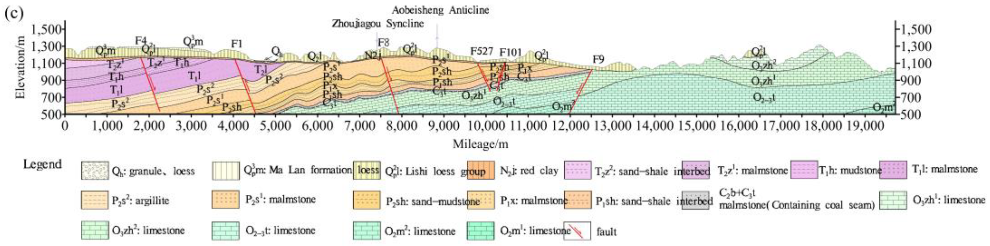
Geologically, the study area is located on the Weibei uplift zone at the southeast edge of the Ordos Basin. As the south side was cut by the east–westward Weihe graben, the area formed transitional imbricated faults and south-rising north-declining fault steps (Figure 1). Folds and faults are developed in this area. The axial direction of the Aibocun-Liuwan anticline, a nearly east–west fold, is consistent with that of the Zaomiao reverse fault. Affected by the Zaomiao fault, the occurrence slopes on the two wings of the anticline are different. North–eastward folds are developed in the area, which are small-scaled and concentrate in the north central area. The Zhaojiayuan anticline is mainly developed in the Sunjiagou formation, and the occurrence slopes on both wings are gentle, forming a complete wide and gentle fold, together with Taimiao syncline. The two wings of the Sanlidong anticline have gentle occurrence slopes. The southeast wing is broken by the Shijiahe fault, but the shape is wide and gentle. The Juntailing syncline has symmetrical wings and gentle occurrence slopes. The Shangliuzhai anticline is an open, flat, and undulating anticline. The core is the Majiagou formation, and the south wing is broken by faults in Dujiayuan area, resulting in discontinuous strata. The Huangbao syncline is in the south of the Shangliuzhai anticline. Its core is the Xiashihezi formation, and its two wings are the Shanxi formation and Taiyuan formation. The Guanjiazui anticline is located to the east of the Huangbao syncline, with the core of the Majiagou formation. Its two wings (the Benxi formation + Taiyuan formation and Shanxi formation) were destroyed by the Chenlubei fault, resulting in different occurrence and incomplete shapes. The Chenlu syncline is in the south of the Guanjiazui syncline, and their tectonic lines are inclined at a large angle. The Chenlu syncline has an obvious incompatible relationship with the lower substructural layers. In addition to these folds, there are the Yuanpan syncline, Zhoujiagou syncline, Xiaodoucun anticline, Majiazhuang anticline, Aobeishen anticline, and Pangjiahe anticline, all of which are short-axis anticlines or synclines. These folds have different axial directions and an uneven distribution.

The faults in the area are relatively developed, mainly normal faults, which can be divided into nearly EW, NE, and NW groups. The details are listed in

Table 1. Information of the faults in the study area.

Code	Nature	Occurrence	Description
F1	Reverse fault	Dipping 70° S	Located in the Yangwan–Zaomiao area, and composed of a series of nearly parallel reverse faults, forming an east–westward compression belt together with the Aibo- Liuwan anticline and syncline.
F2	Reverse fault	Dipping 75° N	Located in the area of Langwoli–Xiabian Village, and developed in the limestone of the Majiagou Formation. Extends eastward, and becomes elusive at Sikuanggou due to coverage.
F3	Normal fault	Dipping S	Located in the area of Qijiashan–Dujiayuan–Xiabian Village, 1.5 km south of the Langwoli–Xiabian Village fault, and merged with the Shijiayuan–Renjiawan fault at Luozhai Village.
F4	Normal fault	Dipping 70° S	Starting from Yangwan in the west, passing through the south bank of Wujiahe River, and ending at the north of Nanguzhai in the east. It is a concealed fault covered by loess.
F5	Reverse fault	Dipping 70° S	Located in the northwest of the Zhaojiayuan anticline. It is a concealed fault covered by loess.
F6	Normal fault	Dipping 55° N	Distributed in the west of Baozibei, extending 2500 m. It is a tensile fault.
F7	Normal fault	Dipping 48° S	Distributed in the east of north Gaojiayuan, extending 2.8 km. It is a tensile fault.
F8	Normal fault	Dipping 75° NE	Distributed in the south of Shijiahe River, as the northern boundary of Taoyuan Mine. The hanging wall is the Shanxi formation and Taiyuan formation, and the footwall is the Shangshihezi formation. It is a tensile fault.
F9	Normal fault	Dipping 75° N	Located in the south of the Huangpu syncline. Starting from Renjiawan in the east and passing Guanjiazui in the south, the fault is composed of two parallel normal faults, and mainly developed in the limestone of the Majiagou formation.
F10	Normal fault	Dipping 65° S	Located in the Liushuwan–Jiaziwo area and composed of two discontinuous faults, the fault has destroyed the upper and lower subtectonic layers.
F11	Normal fault	Dipping 60° SW	Distributed in the area of Dianzipo and Juntailing, extending 3 km.
F12	Reverse fault	Dipping 70° N	Located in the Yujiahe and Huangjiayao areas, east of Wangshiao. The fault is developed in the limestone of the Zhaolaoyu formation and forms a compression fracture zone of nearly 100 m together with east–west folds.

Notes: N, S, and W stand for north, south, and west, respectively.

.

2.2. Lithology

The strata in the study area have complex sedimentary types, showing a typical zonal distribution from southeast to northwest. From bottom to top, the types are as follows: Ordovician (O): Majiagou formation, Taoqupo formation, and Zhaolaoyu formation; Carboniferous (C): Taiyuan formation, Shanxi formation; Permian (P): Xiahihezi formation, Shangshihezi formation, and Sunjiagou formation; Triassic (T): Liujiagou formation, Heshanggou formation, and Zhifang formation; Neogene (N): Jingle group; Quaternary (Q): Jingle formation, Wucheng formation, Lishi formation, Salawusu formation, Malan formation, and modern alluvial diluvium. A small part of the bedrock outcrops and most of it is covered by loess and river valley sediments. Figure 1 shows the lithology distribution of bedrock.

2.3. Groundwater Types

The groundwater in the study area can be divided into the Quaternary loose bed phreatic water, clastic rock fissure water, and carbonate rock karst fissure water. This study focuses on the latter two types. The clastic rock fissure water flows along the joint fissure zone, fault fissure zone, rock stratum, and fold structure zone. Carbonate karst fissure and karst cave are developed in the study area, and become the main occurrence place and channel of karst fissure water. Recharged by densely distributed fissures, karst fissures, and karst caves, karst fissure water joins the runoff of the Tongchuan–Pucheng–Heyang karst water system, running from north to south and from west to east through the fault.

2.4. Physical Characteristics of Rocks

According to the geological data collected in this area, the strata from bottom to top are Ordovician, Carboniferous, Permian, Triassic, Jurassic, Cretaceous, and Quaternary strata. Statistical electrical data and hydrological logging data show that, conglomerate and sandstone have good water bearing capacity and low resistivity, and mudstone is an aquiclude, with high resistivity. The details are listed in

Table 2. Physical properties of the rocks in the study area.

Stratum	Stratum Code	Lithology	Apparent Resistivity Range (Ω.m)	Apparent Resistivity (Ω.m)
Quaternary	Q	Loess	10~50	35
Cretaceous	K	Conglomerate, sandstone, siltstone, mudstone	60~200	120
Jurassic	J	Conglomerate, sandstone with mudstone and coal seam	120~400	250
Triassic	T	Sandstone and mudstone	200~700	360
Permian	P	Sandstone and sandy mudstone	240~850	450
Carboniferous	C	Sandstone and mudstone	300~900	600
Ordovician	O	Limestone and dolomite	500~3000	2000

. The aquifers in this area include quaternary loose rocks, clastic rock fracture, and carbonate fracture, which have a low resistivity. These layers have obvious electrical differences, suitable for electromagnetic exploration and testing.

3. Data Acquisition, Analysis, and Processing

3.1. Audio Magnetotelluric

The geodetic electromagnetic field is generated by the electromagnetic effects around the earth caused by the particle stream and electromagnetic radiation from the sun. The frequency range is wide, from 10⁻⁴ s (10⁴ Hz) to 10⁵ s (10⁻⁵ Hz). The geodetic electromagnetic field sources include magnetic storms, electromagnetic diurnal changes, electromagnetic pulsations, and lightning. Since these sources can be considered infinitely large compared to geological bodies, natural electromagnetic fields are believed to be planar electromagnetic waves perpendicular to the ground, and the propagation of geodetic electromagnetic waves follows Maxwell’s equations [7,8,9,10]. Transforming the Maxwell equation system, we get the homogenous Hermholtz equation satisfying the electric and magnetic fields as follows:

$${\nabla }^{2}E+{\mathrm{k}}^{2}E=0,$$

(1)

$${\nabla }^{2}H+{\mathrm{k}}^{2}H=0,$$

(2)

where $k^2=i\omega \mu \sigma$ is the square of the wavenumber, a complex wavenumber. The complex vector expression of the electric field strength and magnetic field strength can be obtained using Equations (1) and (2) as follows:

$$E=E_0{e}^{ikr},$$

(3)

$$H=H_0{e}^{ikr},$$

(4)

where $E_0$ and $H_0$ are the electric field strength and magnetic field strength at the zero point, respectively, and r is the diffusion distance. From Equations (3) and (4), the electromagnetic field amplitude attenuates exponentially. When it attenuates to 1/e of the ground value, the penetration depth is called the skin depth, which is

$$\delta =\sqrt{\frac{2}{\omega \mu \sigma }}\approx 503\sqrt{\frac{\rho }{f}}.$$

(5)

According to Equation (5), the detection depth is inversely proportional to the square root of the detection frequency and proportional to the square root of the resistivity of the earth medium. When the detection frequency is high, the detection depth is small; as the detection frequency decreases, the detection depth also increases. However, this is an empirical formula [11,12].

3.2. Data Acquisition

The AMT data were acquired using the V5-2000 magnetotelluric observation system produced by Phoenix Corporation of Canada. We used the tensor measurement method to observe the four horizontal electromagnetic field components (Ex, Ey, Hx, and Hy). The power frequency filtering was set as 50 Hz, and the acquisition frequency ranged from 0.35 to 10,400 Hz. In this study, profiles TC1JM and TC3JM were deployed on the existing profiles TC-1 and TC-3 [7], and new profiles, TC-4, TC-5, and TC-6 were deployed in the northwest part of the study area. On the five profiles, there were 110 AMT sites. The direction of the profiles was roughly across to the structural trend (Figure 1).

3.3. Data Analysis

The magnetotelluric method takes the natural plane electromagnetic wave as the field source to obtain the underground electrical information by observing the orthogonal electromagnetic field components on the surface [11,12]. The natural electromagnetic signal is weak and has a wide frequency band. Therefore, under strong electromagnetic interference, the collected data contain electromagnetic noise, resulting in deviated impedance tensor estimation and a distorted Kania apparent resistivity curve [13,14,15,16]. In this section, we apply time–frequency domain analysis on the measured data and summarize the types of resistivity distortion in Tongchuan. Tongchuan City is an important coal production base in Shaanxi Province; thus, the profiles covering the urban area are affected by strong EMI.

AMT site TC211 is in the central area of Tongchuan. As Figure 2a shows, the apparent resistivity phase curve is severely distorted at 1–1000 Hz. At 10–1000 Hz, the distortion is caused by the near source. At 1–10 Hz, the apparent resistivity curve extends downward sharply, and is discontinuous. The time series in Figure 3 contains strong EMI signals, including periodic signals and triangle-like signals; thus, the curves show irregular shapes. It can be inferred that these EMI signals are generated by the shutdown and startup of some large equipment.

AMT site TC402 is surrounded by villages and high-voltage lines. In Figure 2b, the apparent resistivity-phase distortion at 10–1000 Hz is caused by the near-source effect. As shown in Figure 4, the high-frequency part (TS2) of the TC402 time-series curve is affected by periodic EMI noise, and the middle frequency (TS3) part is influenced by the noise similar to Gaussian signal, which has a wide range of influencing frequency bands. The low-frequency part (TS4) has no obvious EMI noise, but the apparent resistivity phase curve is severely distorted, indicating that the Gaussian signal-like strong noise in the middle frequency band can cause serious near-source effect.

The above analysis demonstrates that different types of noise appear intermittently in the low-frequency time series, indicating that the noncontinuous strong noise has a great impact on the resistivity data quality. In the study area, the noise data are mainly distributed in the center and the south area, but less in the north area. In the area within 60 km south to the Tongchuan city, there are Yaozhou District, Fuping County, Sanyuan County, Yanliang District, and the urban area of Xi’an, whereas, in the area within 60 km north to the Tongchuan city, there are only two counties, Yijun County and Huangling County. Therefore, the EMI in the south of Tongchuan City is stronger. In the urban area, the main noise is the PFI, with a frequency range of 10–1000 Hz. At 1–10 Hz, the apparent resistivity curve extends downward sharply, which may be caused by the intensity of magnetic field interference being much greater than that of electric field interference in the urban area. Therefore, this paper uses the dictionary learning method based on sparse decomposition in frequency domain to denois the magnetotelluric data. This method constructs the redundant dictionary atoms matching with common strong electromagnetic interference, and uses the improved orthogonal matching tracking algorithm to separate the strong interference components. This method has good performance in suppressing strong human electromagnetic noise interference in the urban environment [17].

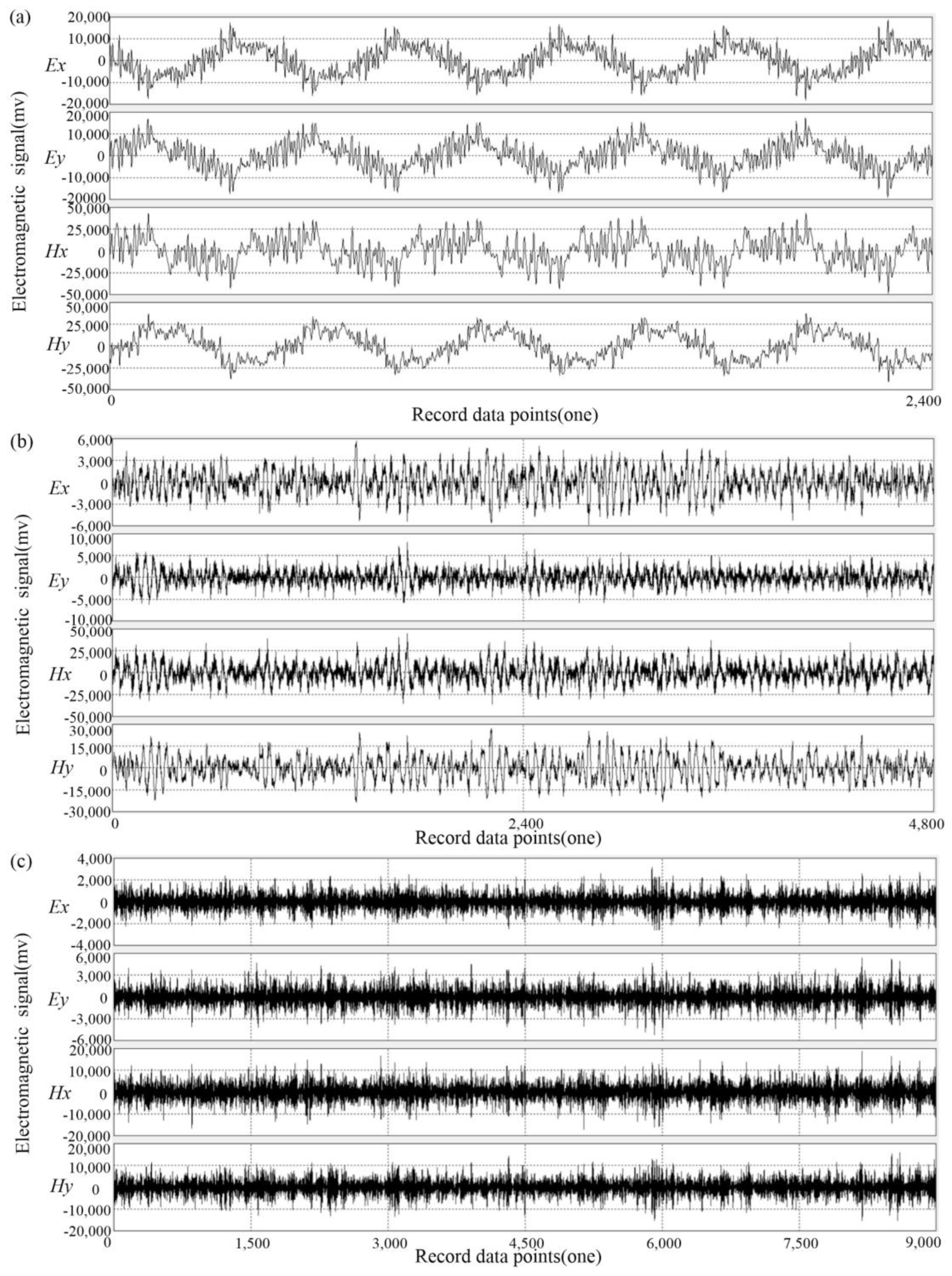
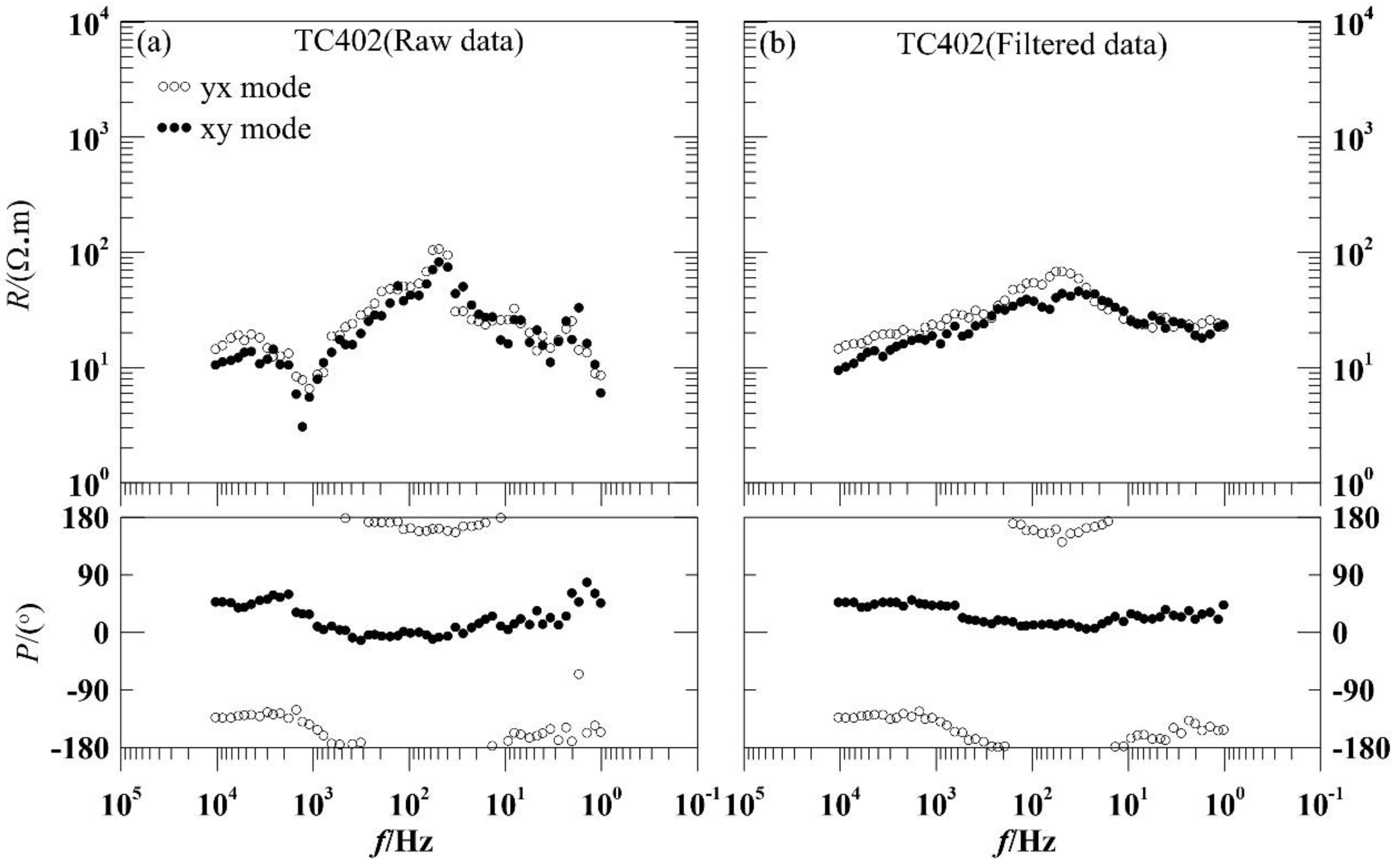
3.4. Data Processing

The AMT data in this study have strong EMI noise of the urban environment, whereby PFI is the main noise [14]. PFI mainly refers to the noise with the frequency of 50 Hz and its harmonic interference. In the time domain, PFI is not zero at each AMT site; however, after the Fourier transform, only a few points are not zero. That is, the harmonic interference has better sparsity in the frequency domain, and its energy is more concentrated in the frequency domain. Therefore, even if the noise is very weak in the time domain, it may be very prominent in the frequency domain. In this study, we apply the fast Fourier transform (FFT) to the AMT time series. After that, in the frequency domain, the redundant dictionary is used to further sparsely decompose the spectrum data using the improved orthogonal matching pursuit (IOMP) algorithm [18]. Obtaining the sparsest representation by two sparse transformations, we can improve the denoising effect [19,20,21].

As shown in Figure 5a, the apparent resistivity phase of AMT site TC211 in all frequency bands is affected by EMI noise, showing many “flying points”. After noise removal using the FFT–IOMP method, the apparent resistivity curve at 1–10 Hz and the “dead band” becomes smooth and continuous (Figure 5b).

In Figure 6a, the curve of TC402 apparent resistivity phase shows a near-source effect at 100–1000 Hz and is not smooth at 1–100 Hz. After removing the noise using the FFT–IOMP method, the curve becomes smooth and continuous (Figure 6b). The above experiments demonstrate that the FFT–IOMP based denoising technology can improve data quality in the urban environment.

4. Analysis on the Inversion Results

4.1. The Initial Inversion Model

In this paper, the two-dimensional (2D) nonlinear conjugate gradient (NLCG) method was used for the 2D inversion of AMT data. This method uses regularization to deal with the minimization problem of objective functions, which obtains the optimal solution of the objective function [22]. Due to the non-uniqueness of inversion, different initial models result in different 2D inversion models. All these inversion models can fit the observation data well. Taking the TC4 profile as an example, this paper adopts different initial models, and compares the results obtained using the generated different 2D inversion models. After that, considering the geological profile analysis, we select the most suitable initial model for AMT data inversion in this study area, to improve the reliability of the 2D inversion results.

Figure 7 shows the results of TC-4 profile inverted using the 2D model with different initial models. Regional geological data show that the shallow layer of the profile is Quaternary loess, with low resistance. The boundary between sandstone and sand shale is located near the section of 2400 m. Due to higher mud content, sand shale has lower resistance compared with sandstone. In Figure 7c, the vertical electrical stratification of shallow Quaternary loess and sandstone, and the horizontal electrical demarcation of sandstone and sand shale are more obvious than those in Figure 7b. In summary, the results of 2D inversion model with a one-dimensional inversion model as the initial model are more reliable.

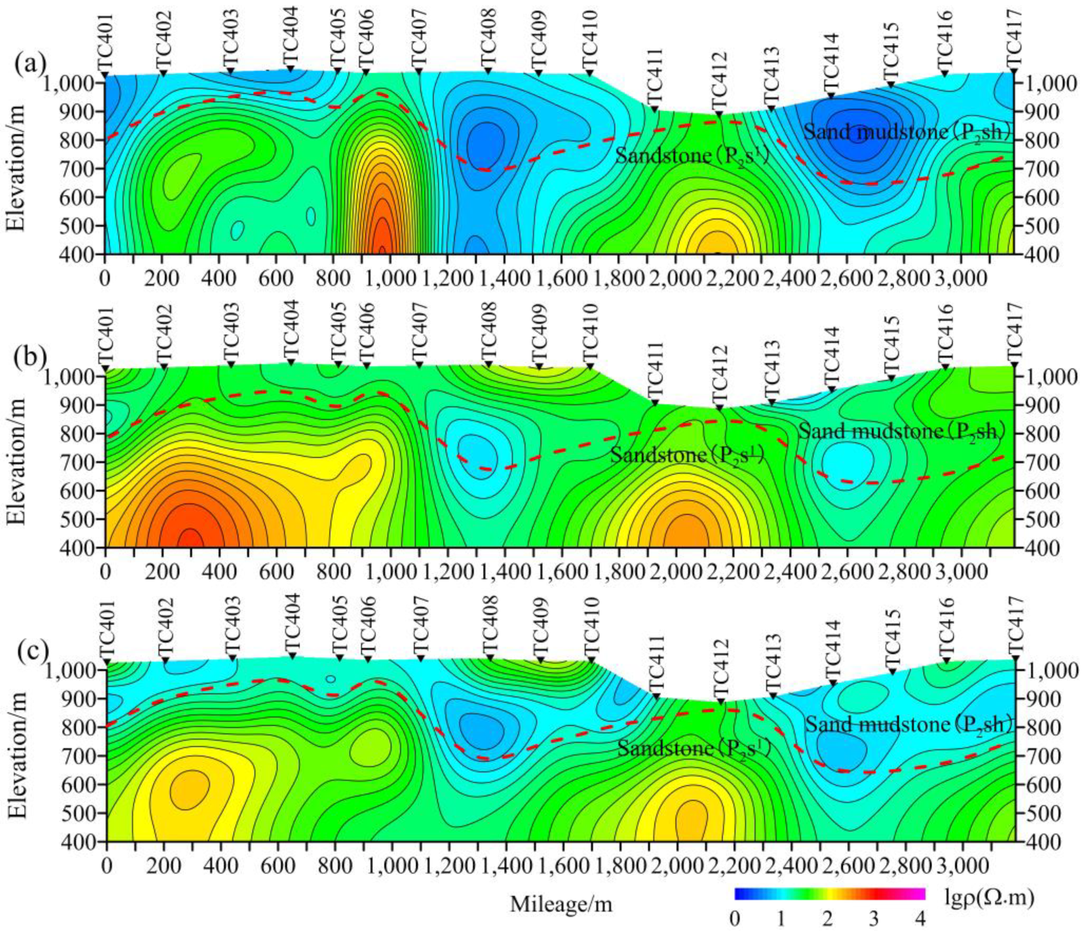
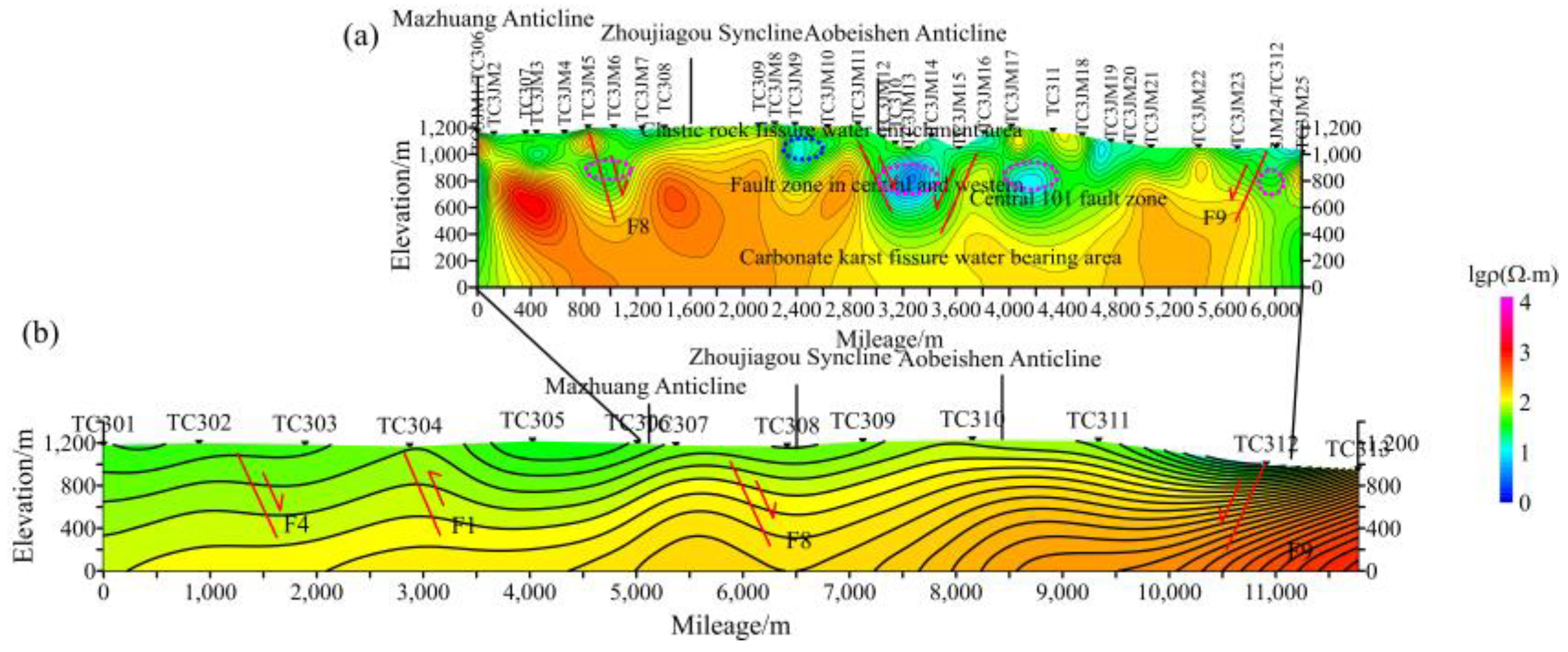
4.2. Analysis on the 2D Inversion Results

In this section, we compare the new profiles (TC1JM and TC3JM) with the original profiles (TC-1 and TC-3) to extract the electrical characteristics of different rocks, for the geological interpretation of the electrical model of the rest three profiles (TC-4, TC-5, and TC-6). The blue dotted line in the inversion results delineates the range of clastic rock fracture water area, and the pink dotted line delineates the range of carbonate karst fracture water area.

TC1JM is the 6200–10,000 m section (AMT sites TC107–TC111) on profile TC-1. As shown in Figure 8a, the bed rock (limestone) in this section is gradually uplifted, which is consistent with the electrical characteristics illustrated by the geological profile B–B’ (Figure 8b). The electrical characteristics of the shallow sandstone stratum on profiles TC1JM and TC-1 are different. The Taimiao syncline is distributed in the section of AMT sites TC1JM3–TC1JM4 (Figure 8a), and its core shows high resistivity. We can infer that the rock mass is compressed and has low water-bearing capacity. The blue dotted line delineates the resistivity contour trap, where the resistivity is low. We can infer that this is an aquifer, with a depth of 200–280 m. According to Figure 8c, the lithology of this layer is sandstone, and the groundwater is clastic rock fissure water.

TC3JM is the 5200–11,400 m section (AMT sites TC306–TC312) on profile TC-3. In Figure 9a,b, the electrical characteristics of fault F8 are the same, but those in the core area of the Zhoujiagou syncline and Aobeishen anticline are different. Generally, the syncline core area has relatively high resistivity due to compression, and the anticline core has relatively low resistivity due to tension. Therefore, the electrical structure shown in Figure 9a is more reliable. In Figure 9a, there are low-resistivity depressions distributed in the 800–1200 m section, which could be controlled by fault F8, resulting in broken rock mass and developed fractures. We infer that this area (delineated by the pink dotted line) has abundant bedrock fissure water at the depth of 300–400 m. At the section from AMT sites TC3JM9 to TC3JM10, the contour gradient reduces; hence, this area (delineated by the blue dotted line) could have abundant clastic rock fissure water. Faults are distributed at the 3000–3600 m and 5900–6100 m sections. Controlled by these faults, the rock mass is broken, and fractures are developed; hence, there is bedrock fissure water (the area delineated by the pink dotted line) at a depth of 300–400 m. At the 4000–4400 m section, a low-resistivity trap is developed in limestone, which could be the karst fissure water.

Profile TC-4 is across the west part of the study area. The Sunjiahe River passes AMT sites TC411–TC412 and is oblique to the profile. As Figure 10 shows, there is a low-resistivity gradient zone at the 1200–1400 m section. Considering the fluctuation of the resistivity contour line, we can infer that a north dipping reverse fault developed here, noted as F5. There are recharge channels between F5 and the Wangjiahe River; thus, F5 has a wide area of low resistivity, which might have clastic rock fissure water (delineated by blue dotted line). At the 2300–3200 m section, the upper area has low resistivity, which may be caused by lithology, rather than fault. According to the regional geological data, the low-resistivity area is sand mudstone, which might have clastic rock fissure water.

Profile TC-5 is distributed in the gully area in the southern part of the study area. The terrain fluctuates greatly, and some regions (AMT sites TC516–TC519) have outcropped bedrocks. As shown in Figure 11, the overlying strata of this profile have low resistivity, with apparent resistivity of 10–70 $\mathsf{\Omega }·\mathrm{m}$, thickness of 0–100 m, and lithology of sandstone and sand mudstone. At the 1300–2300 m section (AMT sites TC507 and TC511–TC512), the resistivity contour depression could reflect the fissure development, resulting in good water storage (area delineated by blue dotted line). At the 1000–1500 m section (AMT sites TC506–TC508) and 1600–2000 m section (AMT sites TC508–TC510), low-resistivity contour traps are distributed at the depths of 450–500 m and 200–300 m. These areas (delineated by a pink dotted line) have abundant karst fissure water. On the profile, the discontinuous area of the transverse electrical structure might be a fault. For example, the section of AMT sites TC502–TC503 could be a reverse fault dipping about 75° north, noted as F2. The hanging and foot walls are limestone. The section of AMT sites TC514–TC515 may be a normal fault dipping 75° south, noted as F3. The hanging and foot walls are limestone.

Profile TC-6 is in the east part of the study area. The bedrock is deeply buried. As shown in Figure 12, at the 900–1750 m section and 2700–3850 m section, the low-resistivity area with a depth of 200–400 m is controlled by faults, resulting in broken rock mass and developed fractures. We can infer that they are clastic rock fissure water-bearing areas. At the 4200–4800 m section, coal mine goaf can be found. Although fault F9 developed in the limestone in this area, the profile shows a wide range of low resistivity, which could be caused by the water filled in the goaf. Therefore, this area has abundant karst fissure water.

In summary, in the study area, the distribution of clastic rock fissure water is determined by sandstone, which has a thick sand layer, a developed structure, and fissures. The regions in the upstream of the river have good conditions for water yield. The development and location of folds and faults are the main factors influencing the distribution of sandstone fissure water in the area. In addition to the lithology and structure, the recharge, accumulation, and discharge of groundwater also have effects on the distribution of fissure water. Without good recharge and discharge conditions, good lithology and structure cannot guarantee good water-bearing capability. Valley areas, which are deeply cut by the river, are low-lying. The river surface water and surrounding bedrock fissure water accumulate here. Such recharge conditions provide good water-bearing capability. Therefore, in the south of the study area, the thin water-bearing sand layer, undeveloped structure, and small groundwater runoff together contribute to the poor water-bearing capability. The occurrence and bearing capability of karst fissure water are mainly controlled by the karst layer and the degree of karst development. The study area on the south of the boundary formed by F2, F3, F9, and F11 is affected by the early structure and karst fissure development; thus, it has strong karst water-bearing capability.

4.3. Analysis of the 3D Inversion Results

The local geological records show that Tongchuan City has complex stratigraphic sedimentary types and well-developed geologic structures. In addition, the 2D inversion of the 3D geological bodies may cause multiple solutions. Therefore, 3D inversion is necessary [23,24]. The 3D inversion requires large computation resources and high-quality original data; hence, we discarded the data severely affected by human interference and selected 65 data from the existing profiles (TC-1, TC-2, and TC-3) and the new profiles (TC1JM, TC3JM, TC-4, TC-5, and TC-6) (Figure 13).

The 3D nonlinear conjugate gradient inversion method takes small data storage and has high calculation efficiency and stable convergence. In this paper, the ModEM inversion algorithm [25,26] is used for the 3D inversion of Tongchuan AMT data. On the resistivity contours of different conductive media, a dense layout, bends, or distortion indicates stratigraphic interface or faults, a sparse and stable layout indicates stable and uniform strata, and undulations mark the stratigraphic interface. Therefore, using the resistivity contour maps of profiles, we can establish an electrical structure model to describe the distribution of underground resistivity along profiles. In this section, combining the local geological data, we slice the 3D electrical model along existing geophysical profiles [1], and we compare the slices with the corresponding 2D electrical models (Figure 14).

As shown in Figure 14a, the upper part of profile TC-1 has low resistivity, reflecting the electric characteristics of Permian and Triassic sandstone and mudstone, and the lower part show high resistivity, reflecting the electric characteristics of Ordovician limestone. The lower part also has some low-resistivity bodies, shown as the lateral segmentation on the profile. The electrical gradient zone indicates faults, suggesting that the folds and fault in the area are developed. Combined with local geological data, the specific analysis is as follows: the 0–3000 m section has low resistivity. Due to the combined contribution of lithology and faults F1 and F4, the rock mass is broken and has good water-bearing capability. At the 2500–3000 m section, the apparent resistivity contour line is uplifted, which could be caused by the Liuwan anticline, where fissures developed at the core. The low resistivity indicates that the anticline has good water-bearing capability.

The 6500–7500 m section shows high resistivity, which could be caused by the Taimiao syncline. Due to compression, the rock mass at the core shows high electrical resistivity. The fractures on the two wings are developed and filled with conductive minerals, showing low resistivity. The local geological data show that the north–northeast extending Zhaojiayuan anticline is distributed in this section, indicating that the nearly east–west extending Liuwan anticline was formed by south–north compression, and it was compressed in the east–west direction later. Therefore, the bedrock on profile TC-3 is dense, and the apparent resistivity is high. An electrical gradient zone is observed at the 8500–11,500 m section. The zone is large, suggesting large faults inside. The local geological data show that the fault is the Shijiahe normal fault (F8). On the two sides of F8, a series of folds and secondary fault structures developed; thus, the rock mass is relatively broken, the fractures are developed, and the stratum has good water-bearing capability. An electrical gradient zone is observed at the 11,500–19,000 m section, which could be the Langwoli–Xiabiancun reverse fault (F2) and Chenlu normal fault (F9). The two faults mainly developed in the limestone of the Majiagou formation. F9 is a large normal fault in the region, which crosses the southern area of the study area from west to east. The 17,000–19,000 m section shows low resistivity, due to the joint effects of F9 and Guanjiazui anticline.

In Figure 15a, the upper part of profile TC-2 has low resistivity, reflecting the characteristics of Permian and Triassic sandstone and mudstone, and the lower part has high resistivity, reflecting the characteristics of Ordovician limestone. The lower part also has some low-resistivity body, demonstrated by the obvious transverse segmentation. The electrical gradient zone represents faults, suggesting that folds and fault structures are developed in this region. A specific analysis considering the local geological data follows.

An electrical gradient zone is present around 2500 m. Under the combined effect of faults F1 and F4, the rock mass developed fissures with good water-bearing capacity. The 8500–11,500 m section has a large range electrical gradient zone, indicating large faults inside. According to the local geological data, the fault is the Shijiahe normal fault (F8), which has a series of folds and secondary faults developed on both sides, resulting in broken rock mass, developed fractures, and good water-bearing capability. In this section, the Yuanpan syncline shows low resistivity on profile TC-1 and high resistivity on profile TC-2. The syncline is formed by compression, showing high electrical resistivity. According to the local geological data, fault F11 developed on the right side of this section on profile TC-4. Obviously, F11 extends northward to the Yuanpan syncline, resulting in rock fragmentation, fissure development, and filling of conductive minerals, causing low resistivity. The 11,500–15,500 m section has high electrical resistivity. An electrical gradient zone is observed around 13,500 m, reflecting the Chenlu normal fault (F9) that mainly developed in the limestone of Majiagou Formation. At the 15,500–18,500 m section, the upper part shows high resistivity, reflecting the core of Chenlu syncline. There are electrical gradient zones developed on both wings of the syncline, indicating developed faults.

In Figure 16a, the longitudinal electrical structure of profile TC-3 is layered, and the transverse electrical structure has a gradient zone. An analysis considering the local geological data follows. At the 0–3500 m section, the apparent resistivity ranges from 100 to 300 Ω·m, the layered structure is not obvious, and no high resistivity is observed in the deep. One possible reason is the similar electrical characteristics of the upper- and lower-part lithology, which is Triassic sandstone and sandstone mudstone, and Permian sandstone and mudstone, respectively. In addition, there is a resistivity boundary at 3500 m, which could be a fault. According to the local geological data, it is the Liuwan normal fault (F4). As shown in Figure 15b, the Liuwan normal fault (F4) and Zaomiao reverse fault (F1) are nearly parallel distributed, and they both developed in Permian sandstone; hence, their electrical properties are similar.

The 3500–10,000 m section has a wide area of low resistivity. The bedrock is deeply buried mainly by sandstone characterized by low resistivity. The local geological data show that the Mazhuang anticline, Zhoujiagou syncline, and Aobeishen anticline are developed in this section, and their axes are roughly parallel. The apparent resistivity contour is gentle, and the apparent resistivity value is low, indicating that the fold formed by the Mazhuang anticline, Zhoujiagou syncline, and Aobeishen anticline is relatively complete, wide, and gentle. An electrical gradient zone is present at the 7000–8000 m section. The apparent resistivity contour of the left part of the zone declines. We infer a normal fault dipping north. According to the local geological data, the fault is the Shijiahe fault (F8). At the section around 11,400 m, the bedrock gradually outcrops, and the apparent resistivity contour on the left side declines. This could be a normal fault dipping north. Considering the local geological data, we can infer that the fault is the Chenlu fault (F9), which mainly developed in the limestone of the Majiagou formation.

The sandstones with high water content are mainly distributed in the central and eastern regions of the study area (Figure 17a). On the other hand, the sandstones in the west and south show relatively high resistivity (Figure 17b), indicating low water content. The bedrock fissure water is distributed in two regions: one is between the Sanlidong anticline and F1 and F4, and the other is between F8 and F9. These areas have low electrical resistivity, indicating that cracks are developed, and bedrock fissure water is relatively developed. In addition, the syncline wing and the anticline core have low electrical resistivity, indicating good water-bearing capacity.

5. Conclusions

In this study, we used the AMT method to detect the groundwater in Tongchuan City, and we obtained the 2D and 3D electrical models. Combined with the local geological data, we characterized the groundwater distribution in the study area, which provides an electrical constraint for the comprehensive understanding of the groundwater distribution, and provides references for deep groundwater exploration in urban areas. The main achievements of the study are as follows:

(1) We analyzed the distribution and types of the electrical resistivity data noise in the study area, and we obtained the noise characteristics. We removed the noise using the FFT–IOMP algorithm to improve the resistivity data quality. The algorithm can also be used to denoise the electromagnetic data in other regions.

(2) We applied 2D and 3D inversion to the AMT data in the study area, and we obtained the 2D and 3D electrical models. We combined the local geological and hydrological data to accurately interpret the geological significance of the electrical models, which lays a foundation for exploring the spatial distribution of groundwater in the study area.

(3) Through analysis, we gained some new understandings of the groundwater distribution in this area. First, the distribution of the clastic rock fissure water aquifer is mainly controlled by folds and faultsm as well as the thickness of sandstone layer, which is generally thick in the north and thin in the south. The water-bearing area is mainly distributed in the middle east of the study area. Second, the distribution of the karst water is mainly controlled by the fracture structure. The Ordovician limestone in the north of the study area is deeply buried and has few fissures, but that in the south gradually outcrops and develops folds and faults, forming the karst water-bearing areas.

References

1. Zhang, Z.J.; Hu, X.; Xie, H. The effect of the application of optimal combination of direct electric sounding method to water exploration in pediment gobi area of th Hexi Corridor. Geophys. Geochem. Explor. 2018, 42, 1186–1193. (In Chinese) [Google Scholar]
2. Gao, P.; Chen, C.; Wang, D. Study on the application of IP sounding in water exploration in desert areas. Ground Water 2020, 42, 134–135+222. (In Chinese) [Google Scholar]
3. Wang, W.; Zhao, Y.; Zhang, Z. Application of nuclear magnetic resonance technology in groundwater exploration. Inn. Mong. Water Conserv. 2018, 11, 16+23. (In Chinese) [Google Scholar]
4. Pan, J.; Zhan, J.; Hong, T.; Wang, H.; Li, Q.; Li, Z. Combined Use of Surface Nuclear Magnetic Resonance and Electrical Resistivity Imaging in Detecting Grondwater. Geol. Sci. Technol. Inf. 2018, 37, 253–262. (In Chinese) [Google Scholar]
5. Wang, K. Application of Transient Electromagnetic Method in Groundwater Exploration in Quartz Diorite Area around a Mine in Eastern Anhui Province. World Nonferrous Met. 2019, 14, 216–218. (In Chinese) [Google Scholar]
6. Lou, B. Application of CSAMT in geology for water. Zhongzhou Coal 2016, 9, 147–150. (In Chinese) [Google Scholar]
7. Xu, Z.M.; Tang, J.T.; Li, G.; Xin, H.C.; Xu, Z.J.; Tan, X.P.; Li, J. Groundwater resources survey of Tongchuan city using audio magnetotelluric method. Appl. Geophys. 2020, 17, 660–671. [Google Scholar] [CrossRef]
8. Song, H.; Xia, F.; Han, P. Effectiveness analysis of ground water investigation by AMT method in Alxa Right Banner. Geotech. Investig. Surv. 2017, 45, 74–78. (In Chinese) [Google Scholar]
9. Bai, Y.; Ji, X.; Guo, W.; Yu, F. Application of Audio Magnetotelluric Sounding Method in Investigation of Groundwater Resources in the Dagler Region. Ground Water 2017, 39, 30–31+64. (In Chinese) [Google Scholar]
10. Wang, J.; Tu, Y. Application of Audio frequency Magnetotelluric Sounding in Geophysical Prospecting in Yili Valley, Xinjiang. Ground Water 2018, 40, 71–74. (In Chinese) [Google Scholar]
11. Tikhonov, A.N. On determining electrical characteristics of the deep layers of the Earth’s crus. Dokl. Akad. Nauk. 1950, 73, 295–297. [Google Scholar]
12. Cagniard, L. Basic theory of the magnetotelluric method of geophysical prospecting. Geophysics 1953, 18, 605–635. [Google Scholar] [CrossRef]
13. Butler, K.E.; Russell, R.D. Subtraction of powerline harmonics from geophysical records. Geophysics 1993, 58, 898–903. [Google Scholar] [CrossRef]
14. Trad, D.O.; Travassos, J.M. Wavelet filtering of magnetotelluric data. Geophysics 2000, 65, 482–491. [Google Scholar] [CrossRef]
15. Cohen, M.B.; Said, R.K.; Inan, U.S. Mitigation of 50–60 Hz power line interference in geophysical data. Radio Sci. 2010, 45, RS6002. [Google Scholar] [CrossRef] [Green Version]
16. Tang, J.; Xu, Z.; Xiao, X.; Li, J. Effect rules of strong noise on magnetotelluric (MT) sounding in the Luzong ore cluster area. Chin. J. Geophys. 2012, 55, 4147–4159. (In Chinese) [Google Scholar] [CrossRef]
17. Tang, J.; Li, G.; Xiao, X.; Li, J.; Zhou, C.; Zhu, H. Strong noise separation for magnetotelluric data based on a signal reconstruction algorithm of compressive sensing. Chin. J. Geophys. 2017, 60, 3642–3654. (In Chinese) [Google Scholar] [CrossRef]
18. Dai, W.; Milenkovic, O. Subspace pursuit for compressive sensing signal reconstruction. IEEE Trans. Inf. Theory 2009, 55, 2230–2249. [Google Scholar] [CrossRef] [Green Version]
19. Li, G.; Liu, X.; Tang, J.; Deng, J.; Hu, S.; Zhou, C.; Chen, C.; Tang, W. Improved shift-invariant sparse coding for noise attenuation of magnetotelluric data. Earth Planets Space 2020, 72, 15. [Google Scholar] [CrossRef] [Green Version]
20. Li, G.; Liu, X.; Tang, J.; Li, J.; Ren, Z.; Chen, C. De-noising low-frequency magnetotelluric data using mathematical morphology filtering and sparse representation. J. Appl. Geophys. 2020, 172, 103919. [Google Scholar] [CrossRef]
21. Li, G.; Gu, X.; Ren, Z.; Wu, Q.; Liu, X.; Zhang, L.; Xiao, D.; Zhou, C. Deep Learning Optimized Dictionary Learning and Its Application in Eliminating Strong Magnetotelluric Noise. Minerals 2022, 12, 1012. [Google Scholar] [CrossRef]
22. Rodi, W.; Mackie, R.L. Nonlinear conjugate gradient algorithm for 2-D magnetotelluric inversion. Geophysics 2001, 66, 174–187. [Google Scholar] [CrossRef]
23. Li, R.; Yu, N.; Wang, X.; Liu, Y.; Cai, Z.; Wang, E. Model-Based Synthetic Geoelectric Sampling for Magnetotelluric Inversion with Deep Neural Networks. IEEE Trans. Geosci. Remote Sens. 2022, 60, 4500514. [Google Scholar] [CrossRef]
24. Yu, N.; Unsworth, M.; Wang, X.; Li, D.; Wang, E.; Li, R.; Hu, Y.; Cai, X. New insights into crustal and mantle flow beneath the Red River Fault zone and adjacent areas on the southern margin of the Tibetan Plateau revealed by a 3D magnetotelluric study. J. Geophys. Res. Solid Earth 2020, 125, e2020JB019396. [Google Scholar] [CrossRef]
25. Egbert, G.D.; Kelbert, A. Computational recipes for electromagnetic inverse problems. Geophys. J. Int. 2012, 189, 251–267. [Google Scholar] [CrossRef] [Green Version]
26. Kelbert, A.; Meqbel, N.; Egbert, G.D.; Tandon, K. ModEM: A modular system for inversion of electromagnetic geophysical data. Comput. Geosci. 2014, 6, 40–53. [Google Scholar] [CrossRef]
Figure 1. The regional geological map and approximate location of Tongchuan study area in China (upper). Geological map of the Tongchuan area (lower). The black triangles are the locations of audio-frequency magnetotelluric (AMT) sites. Geological profiles A–A’ and B–B’ [7] are marked by black lines.
Magnetochemistry 09 00032 g001
Figure 2. Apparent resistivity and phase curve of the data at AMT sites (a) TC211 and (b) TC 402 in the study area.
Magnetochemistry 09 00032 g002
Figure 3. Time series (a) TS2, (b) TS3, and (c) TS4 of AMT site TC211.
Magnetochemistry 09 00032 g003
Figure 4. Time series (a) TS2, (b) TS3, and (c) TS4 of AMT site TC402.
Magnetochemistry 09 00032 g004
Figure 5. Apparent resistivity phase curve of AMT site TC211 (a) before and (b) after noise removal using the FFT–IOMP method.
Magnetochemistry 09 00032 g005
Figure 6. Apparent resistivity phase curve of AMT site TC402 (a) before and (b) after noise removal using the FFT–IOMP method.
Magnetochemistry 09 00032 g006
Figure 7. Inversion results of profile TC-4. (a) Occam 1D inversion model; (b) 2D inversion results with uniform half-space as the initial model; (c) 2D inversion results with Occam 1D inversion model as the initial model.
Magnetochemistry 09 00032 g007
Figure 8. The 2D inversion models of (a) profile TC1JM and (b) profile TC-1 [7]. (c) Geological profile B–B’ [7].
Magnetochemistry 09 00032 g008
Figure 9. The 2D inversion models of (a) profile TC3JM and (b) profile TC-3 [7]. (c) Geological profile A–A’ [7].
Magnetochemistry 09 00032 g009aMagnetochemistry 09 00032 g009b
Figure 10. The 2D inversion result of profile TC-4. The red line marks the locations of faults, and the blue dotted line marks clastic rock fissure water bearing area.
Magnetochemistry 09 00032 g010
Figure 11. The 2D inversion model of profile TC-5. The red line marks the locations of faults. The pink dotted line and blue dotted line delineate the karst fissure water bearing area and clastic rock fissure water-bearing area, respectively.
Magnetochemistry 09 00032 g011
Figure 12. The same as Figure 12, but for profile TC-6.
Magnetochemistry 09 00032 g012
Figure 13. AMT sites selected for 3D inversion. A–A’ and B–B’ are geological profiles.
Magnetochemistry 09 00032 g013
Figure 14. (a) The 2D slice of the 3D inversion results along profile TC-1. (b) The 2D inversion model of profile TC-1 [7]. (c) Geological profile B–B’ [7].
Magnetochemistry 09 00032 g014aMagnetochemistry 09 00032 g014b
Figure 15. (a) The 2D slice of 3D inversion results along profile TC-2. (b) The 2D inversion results of profile TC-2 [7]. (c) Geological profile B–B’ [7].
Magnetochemistry 09 00032 g015aMagnetochemistry 09 00032 g015b
Figure 16. (a) The 2D slice of 3D inversion results along TC-3 profile. (b) The TC-3 2D inversion results [7]. (c) Geological profile A–A’ [7].
Magnetochemistry 09 00032 g016aMagnetochemistry 09 00032 g016b
Figure 17. Spatial distribution of sandstone obtained through 3D inversion: (a) sandstone with high water content and a resistivity of 70 Ω . m ; (b) sandstone with low water content and a resistivity of 200 Ω . m .
Magnetochemistry 09 00032 g017