Article

A Gd-Dimer Benchmark Study: Is DFT an Accurate Method for the Prediction of Gadolinium Exchange Coupling Constants?


1
Institute of Inorganic Chemistry (AOC), Karlsruhe Institute of Technology (KIT), Kaiserstr. 12, 76131 Karlsruhe, Germany
2
Institute of Nanotechnology (INT), Karlsruhe Institute of Technology (KIT), Kaiserstr. 12, 76131 Karlsruhe, Germany
3
Institute for Quantum Materials and Technologies (IQMT), Karlsruhe Institute of Technology (KIT), Kaiserstr. 12, 76131 Karlsruhe, Germany
*
Author to whom correspondence should be addressed.
Magnetochemistry 2026, 12(6), 67; https://doi.org/10.3390/magnetochemistry12060067
Submission received: 27 February 2026 / Revised: 3 June 2026 / Accepted: 8 June 2026 / Published: 10 June 2026

Abstract

Gd(III)-Gd(III) exchange interactions are central to a number of applications, such as the magnetocaloric effect or single molecule magnetism. Broken-symmetry density functional theory is the most widely used computational technique for these calculations, yet no comprehensive benchmark has been established. Here, we present the computational analysis of 27 binuclear Gd(III) compounds in comparison to experimental data and propose a best-practice workflow. We encourage the explicit treatment of scalar relativistic effects and the use of a combination of hybrid functionals with different amounts of exact exchange. Furthermore, we investigated this testbed for structure-property relationships and demonstrated the use of the recommended methodology on two tetranuclear Gd(III) clusters.

Graphical Abstract

1. Introduction

Understanding how paramagnetic ions interact is of utmost importance to understand and predict the properties of multinuclear magnetic molecules. Intramolecular interactions, which are generally much stronger than intermolecular interactions, are responsible for many magnetic properties such as Single Molecule Magnetism (SMM) [1,2,3,4] or the magnetocaloric effect (MCE) used in magnetic refrigerants [5,6,7,8,9,10]. Furthermore exotic spin states such as Single Molecule Toroics (SMTs) can only be realized through such interactions [11,12,13].
Considering that these interactions are responsible for a wide range of properties, they can be determined using a wide range of experiments. In addition to fitting procedures of direct current (DC) magnetometry measurements, which will be discussed in more detail later, the coupling constants can be obtained, for example, from EPR [3], μ-SQUID [14,15,16], and Inelastic Neutron Scattering experiments [17,18,19]. Quantum chemical calculations of these coupling constants are often invaluable to interpret the corresponding data.
In the case of the coupling of lanthanide ions, two major coupling mechanisms need to be considered: magnetic exchange interactions and, in the case of ions with magnetic anisotropy, spin-dipolar interactions [20]. The latter can be obtained from calculations of the magnetic main axes of the individual ions. In contrast, exact values for the magnetic exchange coupling are usually small and difficult to calculate. Studying the magnetic coupling for Gd(III) ions is of particular interest, given their special position in the lanthanide series. As a result of the half-filled 4f-shell, Gd(III) ions do not have any orbital angular momentum and therefore no first-order spin-orbit coupling (SOC). With rare exceptions, they do not exhibit any magnetic anisotropy, and the ground state can be described as a pure S = 7/2 spin state [21]. The lack of a magnetic dipole thus means that two Gd(III) ions can only interact through exchange interaction pathways.
On a technical level, this implies that computational models do not need to treat SOC effects, neither perturbatively nor directly. Scalar relativistic effects generally suffice when calculating Gd(III) compounds [22,23,24]. Consequently, Gd(III) is an important model system to assess the behavior of its spin-orbit coupled neighbors in the periodic table, such as Dy(III), where strong SOC gives rise to significant magnetic anisotropy. This means that the interaction between two Dy(III) ions includes a dipolar contribution in addition to the exchange coupling. Gd(III) ions can thus serve as a model in order to investigate the part of the exchange coupling of this interaction. The measured or calculated magnetic exchange coupling of Gd(III) analogs is often rescaled to the spin of other 4f ions [25], allowing exchange coupling constants calculated on Gd(III) dimers to be transferred to other 4f elements.
The level splitting resulting from exchange coupling can be modeled using a Spin-Hamiltonian approach and a Heisenberg-Dirac-van-Vleck (HDvV) operator. This Hamiltonian describes an effective coupling constant J between two spins S ^ 1 and S ^ 2 [5,10,26].
H ^ = 2 J S ^ 1 S ^ 2
In case of Gd(III) dimers, the energies of the spin states can be described as
E S = J S S + 1 S 1 S 1 + 1 S 2 S 2 + 1   w i t h   S 1 S 2 S S 1 + S 2
with a single variable J. A simple approach to obtain the coupling constant, without calculation of all spin states by multi-reference methods, is Noodleman’s broken-symmetry (BS) approach. Here, the energies of the high-spin (HS) state (S = 7) and the so called broken-symmetry state are successively calculated. To obtain the BS-state, the partially occupied orbitals are localized and “flipped” at a given magnetic center [27]. The resulting wavefunction is not a spin eigenfunction but a linear combination of all possible spin states with alpha and beta spin densities localized at one of the two Gd(III) centers, respectively. From the BS and the HS states, the effective coupling constant J can be calculated using a formula proposed by Yamaguchi [28].
J = E H S E B S < S B S 2 > < S H S 2 >
The advantage of the BS approach is that DFT can be used to calculate the energies of these two electronic states which are represented by single determinants. In fact, BS-DFT calculations on Gd(III) multinuclear compounds have been standard practice for over 20 years [29,30]. However, the coupling constants are usually rather small, and the calculated values depend on the respective density functional. Therefore, the calculated coupling constants are often not in agreement with the experimental data. This raises the question of whether DFT is a useful method to predict Gd(III) exchange coupling constants.
Previously, BS benchmark studies have been performed on Cu(II)-dimers and suggest a strong dependence of the resulting coupling strengths on the functional and, particularly, on the amount of exact Hartree-Fock exchange [31,32,33,34,35]. There are indications that range-separated functionals perform slightly better than hybrid functionals [36]. Furthermore, multi-reference calculations do not always significantly improve the results obtained by DFT [37,38]. Similar conclusions have been drawn with respect to exchange coupling constants of mixed 3d-4f complexes, mainly Cu(II) and Gd(III) [39,40] but also combinations with other 3d-metals [41,42,43,44] and organic radicals [45].
To the best of our knowledge, no comprehensive benchmark study has been performed to gauge how different parameters in the calculations influence coupling constants for Gd(III) dimers obtained using BS-DFT. In comparison to pure Cu(II)-dimers, investigating Gd(III) requires another dimension in the calculation, which is the treatment of relativistic effects. This and the influence of the basis set have been the subject of several studies in the past, concluding that an explicit treatment of scalar relativistic effects is required, while the choice of basis sets plays only a minor role [23,46].
For Gd(III) dimers, Rajeshkumar et al. concluded that there is a very minor functional dependence and that both pure and hybrid DFT calculations yielded similar results for a set of carboxylate-bridged dimers [24]. However, there is still no broad theoretical study to determine the limit of BS calculations, and no best practices have been established. The present study aims to fill this gap. The important question is whether, given the small size of the magnetic exchange interaction for 4f-compounds, a procedure can be established for Gd(III) dimers (DFT functional, treatment of scalar relativistic effects, basis set) which yields quantitatively correct size and sign of the magnetic exchange coupling constants as obtained in experiment.

2. Testbed Molecules

In total, 27 dinuclear Gd(III) complexes were chosen for this benchmark study. All compounds were chosen to meet the following criteria. They should:
  • Only have one crystallographic distinct molecule in the unit cell.
  • Include exactly two paramagnetic Gd(III) and no other paramagnetic ions.
  • Cover a wide range of bridging modes and different bridging atoms in order to capture possible changes in the electronic structure as a result of the different nature and different distortions of bridging units. The latter is known to have a significant influence on both the sign and the strength of exchange coupling in transition metal compounds as described by the Goodenough-Kanamori-Anderson rules [47,48,49].
  • Be magnetically characterized with at least DC SQUID measurements in order to get experimental reference values.
  • Cover a wide range of both ferromagnetic and antiferromagnetic interactions.
Using these criteria, the 27 molecules summarized in Table 1 were selected. The molecular structure of each molecule is depicted in Figures S1–S3.
The selected set of compounds features a wide range of molecules with intramolecular Gd-Gd distances between 3.246 Å and 4.316 Å. These include neutral, anionic, and cationic complexes, compounds with antiferro- and ferromagnetic coupling, as well as mixed-metal compounds featuring diamagnetic Zn(II) ions.
Most Gd(III) dinuclear compounds reported in the literature involve oxygen-based bridges, which are mirrored in the compounds selected for this benchmark study. Since there is such an abundance of O-bridged Gd(III) dimers, an emphasis is put on investigating the different types of oxygen-based bridges. The compounds studies here thus include dimers bridged by hydroxides ((20),(25)), alcoholates ((9), (11)–(15), (17), (21), (22), (26), (27)), carboxylates ((4), (13)–(16), (18)–(20)), carbonates ((10), (24)), nitrates ((11)) and phosphonates ((23)). In addition, compounds with bridging units based on different elements are featured with two molecules bridged by carbon atoms (1) and (2), each molecule bridged via S- and N-based ligands ((3) and (8)) as well as four compounds with bridging chlorido ligands (4)(7).
A range of different fitting algorithms and Spin-Hamiltonians were used in the papers reporting these compounds. For consistency, the original magnetic data from the publications were re-fitted here using uniform procedures.

3. Computational Workflow

The crystal structures were taken from the published crystallographic information files (CIF). In the cases where structures are refined with disorder, only the majority disorder component was chosen as a model. Any lattice solvent and counterions are generally neglected. In the first step, both Gd(III) were replaced with Y(III), and a geometry optimization of the hydrogen positions was carried out at the b3-lyp/def2-TZVP level of theory [75,76,77,78,79] using the rij-approximation [80,81] and d4-dispersion correction [82,83] in TURBOMOLE 7.7.1 and 7.8 [84,85]. This was necessary since, in contrast to the positions of other atoms, bond lengths to hydrogen atoms are generally underestimated in SC-XRD. The optimized geometries are supplied as xyz-files in the Supplementary Materials.
Ab-initio multi-reference calculations were performed on all Gd(III) centers individually to extract the crystal-field parameters for fitting. As these parameters are defined for each ion individually, two calculations were performed for every molecule. In each calculation, one Gd(III) ion was replaced by Y(III), and the properties of the remaining Gd(III) ion were calculated. The molecule was translated for the Gd(III) position to coincide with the origin. Firstly, the magnetic orbitals were optimized. To do so, a DFT calculation was performed using the b3-lyp functional, an x2c-TZVPall all-electron basis [86] for the metal ions and a def2-TZVPall basis for all other atoms. Relativistic effects were treated through one-component X2C-theory [87]. Additionally, the rij approximation was used, as well as a grid of size 5 and Fermi smearing for reliable convergence. Next, the singly-occupied natural orbitals were chosen as the active space for Restricted Open Shell Hartree Fock (ROHF) calculations using a local version of TURBOMOLE by C. v. Wüllen. Here, the fourth-order Douglass-Kroll Hess approach was chosen to treat relativistic effects [88,89]. A Complete Active Space Spin Orbit Configuration Interaction (CASOCI) [90] calculation was performed by diagonalizing the full CI spin orbit coupled Hamiltonian within the active (7 in 7) space using a Davidson algorithm to extract the lowest 100 states. The energies of the 8 states associated with the 8S7/2 ground state of Gd(III) as well as the extracted Extended Stevens Operators (ESOs) are summarized in the SI, Tables S1–S15. The largest splitting was calculated as 2.01 cm−1 for the highest KD of the ground state in compound (2). Even at low temperatures, this KD will be significantly populated, which corroborates that, for DC-SQUID measurements (usually T ≥ 1.8 K), the approximation of Gd(III) ions as isotropic is reasonable.
Single-point broken-symmetry calculations were then carried out on each structure with the functionals and basis sets described below. Unless otherwise mentioned, the rij-approximation was used. Using Natural Population Analysis (NBO), it was confirmed that each Gd(III) ion carries approximately seven unpaired 4f-electrons. In general, the energy is converged to 10−9 Eh and the density to 10−7. The conversion factor from Eh to cm−1 is assumed to be 220,000. The coupling constants are calculated using the above-mentioned Yamaguchi formula [28]. Using this methodology, coupling constants are converged to approx. 10−5 cm−1.

4. Fitting Procedures

The extraction of exchange coupling constants from the magnetic susceptibility is routinely done through various fitting procedures. One such approach is derived from the van-Vleck equation [91].
χ m = N A n E n 1 2 k T 2 E n 2 e x p E n 0 k T n exp E n 0 k T
This approach expands the energy as a power series with respect to magnetic field. Introducing an HDvV operator and simplification for a spin system with two S = 7/2 spins leads to a Bleaney-Bowers equation, which can be fitted to the experimental data [92,93].
χ m T = 2 N a μ B 2 g 2 k e x p 2 J k T + 5   e x p 6 J k T + 14   e x p 12 J k T + 30   e x p 20 J k T + 55   e x p 30 J k T + 91   e x p 42 J k T + 140   e x p 56 J k T 1 + 3   e x p 2 J k T + 5   e x p 6 J k T + 7   e x p 12 J k T + 9   e x p 20 J k T + 11   e x p 30 J k T + 13   e x p 42 J k T + 15   e x p 56 J k T
Another possibility is to use the program PHI published by Chilton et al. [94], which includes the Lines model [95] to fit magnetic data. Here, the isotropic coupling between two ground-state multiplets is calculated exactly, while excited multiplets only experience an effective field [96]. Lastly, it is possible to consider a small Zero Field Splitting (ZFS) for each Gd(III) ion. The Stevens-Parameters [97,98] parametrizing the ZFS can be calculated using the CASOCI program published by some of us [90]. A first step of the here presented study was to gauge how comparable these three different fitting procedures are.
The results of all employed fitting schemes are summarized in Tables S16–S18 in the SI. Importantly, we find that there is no significant difference between the results using the different fitting procedures. This means that for Gd(III) ions, it does not matter which one of the mentioned fitting methods is employed. For all 27 compounds, a good fit could be obtained without the need to introduce crystal field splitting. The final reference values for the testbed here are those fitted with the Lines model as integrated in PHI [94], including the ZFS, as shown in Table 2.

5. Results and Discussion I: Influences of DFT-Options

We successively tested general DFT options for their influence on the calculated exchange coupling constants. In a first step, we investigated the basis set dependency, followed by an analysis of the treatment of relativistic effects, the possibility of diffuse basis functions, and the grid size. All calculations in this section were performed using the bh-lyp [76,77,79] functional and the rij-approximation. Scalar relativistic effects are treated with X2C.
In order to investigate the influence of the basis set, we used various locally dense basis sets. The atoms of each molecule were divided into three groups: (1) the Gd(III) ions, (2) all other non-hydrogen atoms, and (3) the hydrogens. For each group, the basis set was varied independently. Since it is the most important group in this study, a large number of basis sets were tested for the Gd(III) ions, namely x2c-SVPall, x2c-TZVPall, x2c-TZVPPall, x2c-QZVPall, and x2c-QZVPPall [86,99]. For the second group of atoms, x2c-SVPall, x2c-TZVPall, and x2c-TZVPPall basis sets were tested, and the small basis sets x2c-SV(P), x2c-SVP, and x2c-TZVP were used for the hydrogen atoms. This amounts to 45 calculations per molecule, the results of which are summarized in Tables S19–S24 in the Supplementary Information.
For conciseness, the basis sets will be abbreviated only by their level. In order to compare the results of individual calculations, the calculation using the largest basis QZVPP-TZVPP-TZVP is chosen as a reference value. Next, the error of each calculation with respect to this reference value is determined. The calculations of each basis-set combination for each of the 27 compounds are averaged to give a Mean Absolute Error (MAE) for each basis set combination. These MAEs, as well as their standard deviations, are summarized in Table S25. In Figure 1, the MAE values are displayed by keeping the basis sets of two of the three groups of atoms fixed while varying the third (varying the Gd(III) ion basis sets in the left column, the non-hydrogen atom basis sets in the middle column, and the hydrogen atom basis sets in the right column). The varied basis sets are indicated on the x-axis.
While the MAE for the smallest basis set combination (SVP-SVP-SV(P)) is only ca. 0.007 cm−1, already close to the experimental accuracy, it can be significantly further reduced using larger basis sets for both the Gd(III) ions and the non-hydrogen atoms of the ligands. No significant differences were observed on varying the basis set used for the hydrogens, so that basis sets larger than the smallest one tested here (x2c-SV(P)all) are unnecessary for this specific application. However, it is clear that split-valence (SVP) basis sets are an inadequate choice for all but the hydrogen atoms. Increasing from a triple-ζ basis to a quadruple-ζ basis leads to small changes for the metal, far smaller than experimental accuracy. Furthermore, it should be noted that the choice of basis set affects compounds (1) and (2) more than all other molecules (by a factor larger than 10). Excluding these two will reduce the MAE for the smallest basis set from 0.007 cm−1 to 0.004 cm−1, as seen in Table S25. A similar effect can be reported for the standard deviations.
In summary, we suggest the use of triple-ζ basis sets for all non-hydrogen atoms for a reasonable cost-accuracy balance. As the basis set for the hydrogen atoms does not have any influence on our testbed, the smallest possible basis set suffices. Consequently, unless mentioned otherwise, the basis set of choice will be x2c-TZVPall for all non-hydrogen atoms and x2c-SV(P) for hydrogen. The expected error of this choice is ca. 3 10−4 cm−1. This error is well below DFT and experimental accuracy.
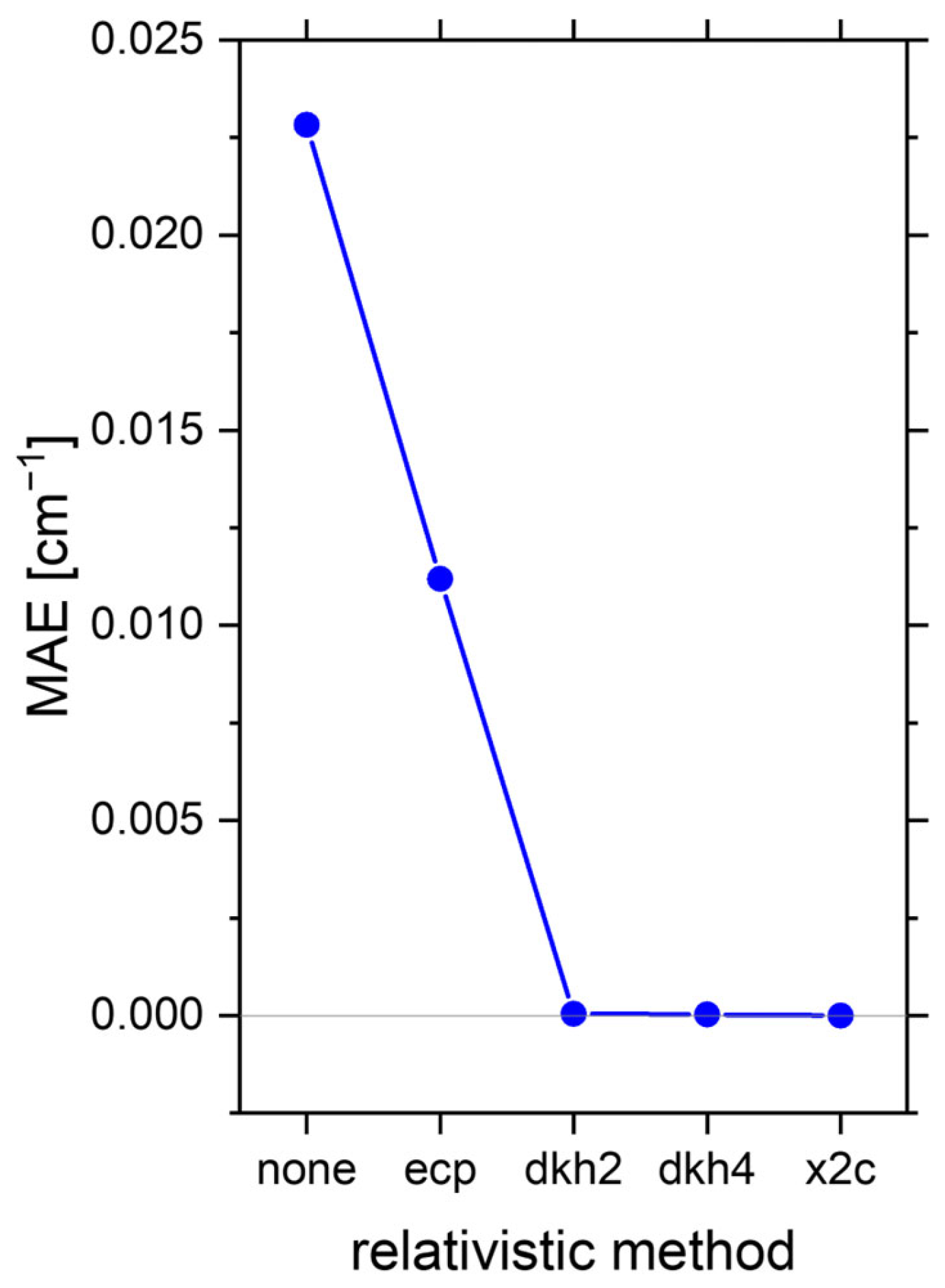
Having established the optimal basis set combination, the influence of the relativistic treatment was then investigated. Keeping the bh-lyp functional, the rij-approximation, and the basis set fixed, the relativistic method was altered. We have chosen five methods which we compare here: (i) not treating relativistic effects at all, (ii) using Effective Core Potentials (ECPs) as included in the def2-basis set series, (iii) and (iv) the all-electron treatments 2nd and 4th order Douglass Kroll Hess (DKH2 and DKH4), and (v) exact decoupling (X2C). The calculated coupling constants, as well as MAEs and standard deviations, are summarized in Table S26. The MAEs with respect to X2C are shown in Figure 2. It can immediately be noted that large errors occur when there is no treatment of relativistic effects. Furthermore, ECPs were shown to be unreliable. DKH2, DKH4, and X2C were found to give very similar results, and DKH2 was therefore used for all further calculations since it is the computationally least expensive method of the three.
In a third step, grid sizes of 3, 4, 5, and 6 have been tested for their influence on the coupling constants. The MAE for the coarsest grid tested (3) with respect to the finest grid size tested (6) is smaller than 10−4 cm−1. The coupling constants and MAE are summarized in Table S27. In this study, a fine grid 5 will be used in case other functionals are more strongly dependent on the grid.
Finally, one diffuse p, d, and f function was included in the Gd-basis. Since these are not optimized for x2c-TZVPall, the diffuse functions from the def2-TZVPDD basis were used. Because no auxiliary basis functions are available for this custom basis, the rij-approximation could not be used. The coupling constants are summarized in Table S28. The mean absolute difference to the x2c-TZVPall basis without diffuse function is 3 10−4 cm−1. Consequently, we conclude that diffuse functions have no noteworthy influence on the coupling constant.
In summary, the following calculations will be performed using the smallest available split-valence basis for hydrogen and a triple-ζ all-electron basis for all other atoms. Relativistic effects are treated with second-order DKH.

6. Results and Discussion II: Influence of the Exchange Correlation Functional

The values of DFT-calculated exchange coupling constants are known to be extremely dependent on the chosen functional. Thus, we have chosen 25 DFT-functionals which are tested here for their performance in reproducing the coupling constants obtained from fitting the experimental data. This test set contains three LDA (s-vwn [100,101], pwlda [102]), four GGA (b-lyp [77,79], b-vwn [77,101], b-p [77,101,103], pbe [102,104]), three meta-GGA (tpss [102,105,106], rev-m06-L [107], scan [108]), nine hybrid-functionals (b97 [109], b3-lyp [76,77,78,79], bh-lyp [76,77,79], bhandhlyp [76,77,79], tpssh [77,102,105,106], tpss0 [105,106,110], pbe0 [102,104,111,112], m06 [34], m06-2x [34]) and three range-separated hybrid functionals (cam-b3lyp [113], ωb97 [109,114], ωb97-x [109,114]). More recent developments, including three local hybrids (tmhf [115], chyf [116], lh07tsvwn [101,117]) and one range-separated local hybrid (ωlh23tde [118]) were tested as well. These functionals allow for the examination of different influences, such as the position on the Jacob’s ladder, the influence of exact exchange, and the correlation functional.
The results of all calculations are summarized in the Supplementary Information, Tables S29–S34. We want to note that the S 2 -expectation values (Tables S35–S46) of HS- and BS-states indicate no notable spin polarization. For (1) and (2), the deviation from the expected values is still small but one order of magnitude larger than for all other compounds.
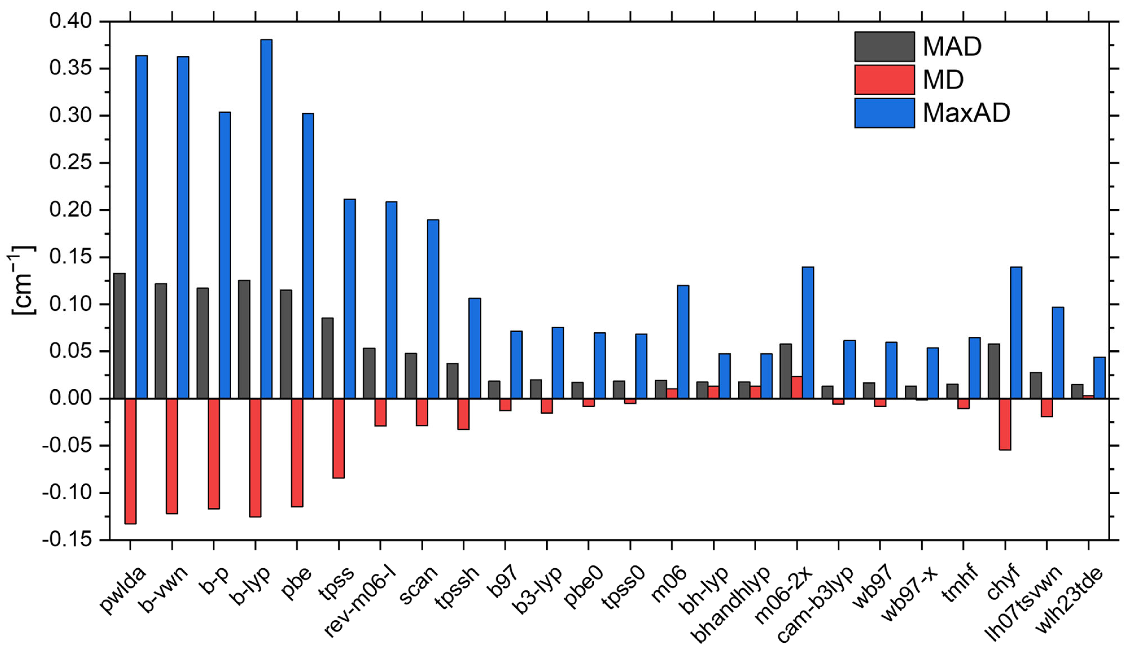
To enable simpler comparison and use the experimental reference data from Table 2, we will use three criteria of accuracy: The Mean Absolute Deviation (MAD) is calculated as the mean absolute difference to the experimental values. The Mean Deviations (MD) to the experimental values are calculated without taking the absolute value of the errors and can therefore be negative. The Maximum Absolute Deviations (MaxAD) for each functional with respect to the experimental values are shown as well. These are summarized in Figure 3 and Table S47. Root mean squared deviations (RMSD) penalize large errors more strongly and are also computed for completeness in Table S47. Compounds (1) and (2) were excluded from this investigation, and their very different behavior is investigated separately below. Furthermore, a peculiarity is observed for the m06-calculation of compound (8), which is deviating significantly from the trend of the other 24 molecules in the remaining testbed, with a deviation of 1.8 cm−1 in comparison to the experimental value. A possible reason for this will be discussed later.
The results shown in Figure 3 suggest that LDAs and GGAs are not suitable, given the large MAD values of more than 0.1 cm−1. While meta-GGAs generally perform better, they still give rather large MADs of ca. 0.05 cm−1. Better accuracy in terms of reproducing the experimental coupling constants is obtained using hybrid functionals. The functionals pbe0, bh-lyp, and bhandhlyp all have a MAD of 0.017 cm−1, b97 and tpss0 0.018 cm−1, and b3-lyp 0.020 cm−1. Exceptionally good results can be obtained using range-separated functionals such as cam-b3lyp (MAD = 0.013 cm−1) and ωb97-x (MAD = 0.017 cm−1). For local hybrids, tmhf is the best performing functional (MAD = 0.015 cm−1). While the range-separated local hybrid functional ωlh23tde performs well (MAD = 0.014 cm−1), the great computational demand meant that a number of calculations did not converge within 30 days on 6 CPUs.
Although these numbers might seem encouraging, it has to be considered that the MaxAD-values obtained from this testbed are between 0.04 cm−1 and 0.08 cm−1 for the aforementioned well-performing functionals, and so of similar magnitudes as the coupling constants themselves.
To test the influence of the correlation functional, a number of functionals with the same exchange but different correlation terms were included in the test set. The LDAs s-vwn and pwlda both use a Slater exchange in combination with correlation as suggested by Vosko, Wilk, and Nuisair [101] or Perdew and Wang, respectively [102]. In this benchmark, the resulting MADs are very similar (0.132 cm−1 and 0.133 cm−1), suggesting only a minor influence of the correlation term. A similar conclusion can be drawn comparing the GGAs b-vwn, b-p, and b-lyp, which all calculate the exchange energy using the exchange expression published by Becke in 1988 [77]. Again, the differences in MADs between the three functionals are smaller than 0.01 cm−1. Consequently, the contribution of correlation to this interaction can be assumed to be minor with respect to the exchange.
Furthermore, when comparing hybrids with their corresponding non-hybrids, a general increase in accuracy can be reported. This correlates with an increase in exact (Hartree-Fock) exchange. The hybrid functional tpss0 (25% HF) performs better than tpssh (10% HF) which in turn performs better than the meta-GGA tpss. The same can be observed on comparing the hybrid pbe0 with the pbe functional. The M06-functional suite is unusual in that the hybrid m06-2x (54% HF) and the meta-GGA rev-m06-L both perform worse than the hybrid with lower exact exchange m06 (27% HF). The largest family investigated was that using B88-exchange with the GGAs b-lyp, b-vwn, b-p as well as the hybrids b3-lyp, bh-lyp, bhandhlyp, and the range-separated cam-b3lyp. Again, all hybrids perform better than the GGAs, and the hybrids with a larger amount of exact exchange perform better than those with lower. Overall, we note that cam-b3lyp outperforms all other functionals with regard to the MAD values.
The previous discussion raises the question about the role of the amount of HF-exchange. To investigate this, we started with the well-known semiempirical b3-lyp functional which takes the form
E x c = A E x H F + 1 A E x S l a t e r + B E x B 88 + C E c o r r V W N V + 1 C E c o r r L Y P
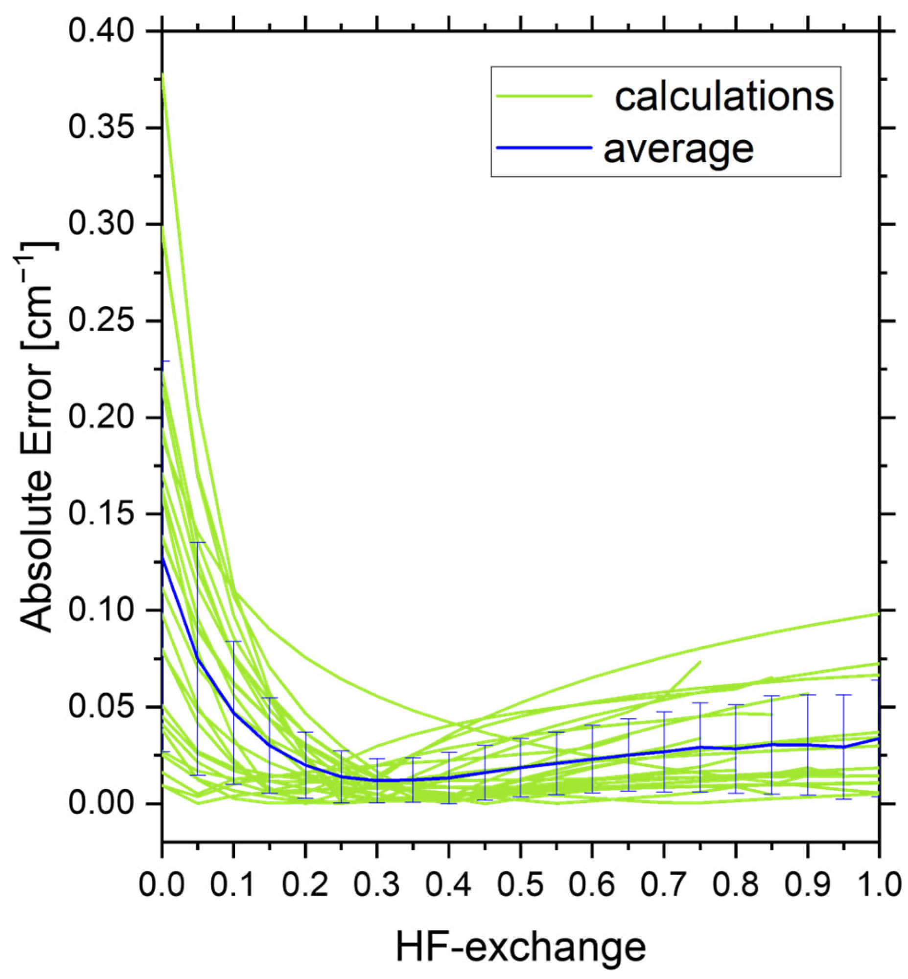
In the classical b3-lyp functional, the variables A, B and C are 0.2, 0.72 and 0.19 respectively. In this study, we kept the parameters B and C fixed, while scaling A from 0 (no HF-exchange) to 1 (no Slater exchange). The results of these variations in A are summarized in Tables S48–S53. Figure 4 shows the absolute errors with respect to the experimental values for all molecules but (1) and (2), which again show a significantly different behavior and are therefore excluded.
When going to higher HF-exchange contributions, a number of calculations become unstable where formally doubly occupied orbitals form open-shell singlet states. Therefore, spin density occurs on the ligands, leading to non-physical results (Figures S4 and S5, Table S54). This happens above 65% for compounds (12) and (21), which are the earliest occurrences of this. Secondly, it is important to recognize that each of the molecules in this testbed has a unique amount of exact exchange needed for the best fit to the experimental data. Consequently, there is no global amount of exact exchange that would minimize the error for all molecules simultaneously. Between 30–35% exact exchange; however, the mean absolute error is minimized at only 0.012 cm−1. The MAE curve around this minimal value is rather flat, with MAE values lower than 0.02 cm−1 between 20% and 50% of HF-exchange. This coincides with the compositions of the best-performing abovementioned hybrid functionals. Interestingly, this minimum value is very similar to the optimal amount of exact exchange suggested for other spin centers, e.g., for NiO investigated by Moreira et al. in 2002 [119].
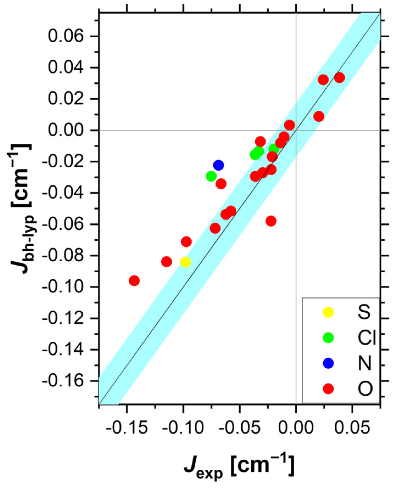
Therefore, we suggest the use of four functionals, namely bh-lyp (or bhandhlyp), pbe0, cam-b3lyp, and ωb97-x. These functionals have performed well in the benchmark, and importantly the pbe0 functionals contain a slightly lower, while bh-lyp contains a larger, amount of exact exchange than the optimal 35%. In the next section, we will show the graphs for bh-lyp, considering that a range-separated hybrid might be too computationally expensive for certain applications with large molecules. The performance of these four functionals against the experimental values is visualized in Figure 5 and Figure S6. As expected, a clear linear correlation can be observed. Linear regressions are calculated for the four suggested functionals and an average of them, summarized in Figure S7. In this benchmark study of Gd(III)-Gd(III) couplings, cam-b3lyp was identified as the best functional with an R2-value of 0.86 and a slope of 0.998. In contrast, bh-lyp, cam-b3lyp, and ωb97-x were found to slightly underestimate the magnitude of the coupling (slopes < 1), while pbe0 slightly overestimates it.
So far, we have investigated general trends over the whole set of compounds. However, a common application could be to rationalize the differences between chemically similar compounds. In compounds (13), (14), and (15), the Gd(III) ions are coordinated by similar ligands, but vary significantly in their fitted coupling constants with −0.062 cm−1, −0.022 cm−1, and −0.014 cm−1, respectively [62]. The four suggested functionals give a range between −0.054 cm−1 and −0.086 cm−1 for compound (13). The range calculated for compound (14) is −0.058 cm−1 to −0.092 cm−1, and −0.008 cm−1 to −0.013 cm−1 for compound (15). Thus, the measured coupling constants for compounds (13) and (15) are captured well by DFT. However, the calculated coupling strength for compound (14) is very similar to the value of (13), at odds with the experimental value. From the DFT perspective, compounds (13) and (14) are structurally almost identical, with similar Gd(III)-Gd(III) distances of 3.88 Å and 3.87 Å, and Gd(III)-O-Gd(III) bond angles of 106.8° and 106.5°. This is in line with a study by Roy et al., which has shown that the influence of residues at acetate bridges is minor [30]. We want to point out here that the S 2 expectation values for (13) and (14) are almost identical, and there is no indication of an unusual electronic situation. Furthermore, (14) is responsible for 9 out of 25 maximum deviations with experiment in Figure 3 (Table S55), indicating the worst performance with the exception of (1) and (2). We believe these outstanding errors may indicate an issue with the experimental data. Therefore, it remains unclear why the experimental values of (13) and (14) are so different.
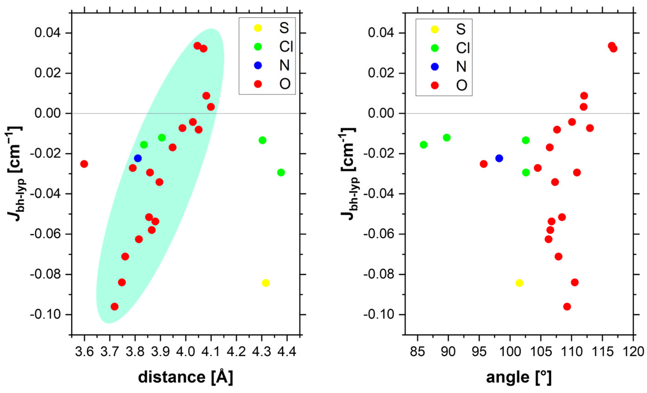
Finally, we revisit the previously suggested structure property relations by plotting the coupling constants calculated here against the angles and distances of the testbed molecules. Here, we compare whether such relations can be transferred to a structurally diverse set of compounds. All graphs for the best four functionals can be found in the SI, Figures S8 and S9. The results for the bh-lyp functional are summarized in Figure 6. As apparent from these figures, compounds with Gd(III)-Gd(III) distances between 3.7 Å and 4.2 Å show a clear correlation to the calculated coupling constants. The same correlation can be reported for the other three functionals as well as the experimental fits. Importantly, this suggests that similar exchange pathways are active in these molecules, whereas other mechanisms become dominant in compounds (3), (5), (6), and (26). These show significant coupling at larger distances and weaker coupling for shorter distances. The possibilities for such alternative mechanisms are discussed in the following section. Furthermore, no noteworthy difference between the coupling in carboxylate and alcoholate-bridged dimers can be reported.
In contrast to this clear correlation in terms of Gd(III)-Gd(III) distances, no such trend can be observed for the Gd(III)-Ligand-Gd(III) angles. This is at odds with previous findings on lanthanide compounds, suggesting that the angle is the most important parameter [24]. The difference is that different bridges are included in our study, while the dependence on the bridging angle is usually investigated within one type of bridge.
This can be supported by calculating the correlation coefficients between the distance, the smallest bridging angle, and the calculated constants. We used Spearman’s [120] and Pearson’s [121] correlation coefficients. While Spearman’s method is purely rank-based, so it is only dependent on the ordering of the magnitude of the data points, Pearson’s method assumes a linear correlation function. We find no correlation between the distances and angles in our data set, which includes various bridging units. Furthermore, the correlation coefficients between the angle and calculated coupling constant are insignificant for O-, N-, S-, and Cl-bridged Dimers combined (rS = 0.31; rP = 0.15) and the subset only including O-bridged dimers (rS = 0.44; rP = 0.24). The correlation between the Gd(III)-Gd(III) distance and the calculated coupling is larger for all molecules shown in Figure 6 (rS = 0.53; rP = 0.34) but still insignificant. The only significant correlation can be reported for the distance-J correlation in the subset of O-bridged dimers with rS = 0.84 and rP = 0.77. This supports the aforementioned statements.
At this point, we want to stress that this does not mean that a strong correlation could exist between structures with very similar bridging motifs, such as the previously investigated bridge with two alcoholates [24]. In fact, one can find a strong correlation between bridging angle and exchange interaction only comparing compounds (9), (12), (17), (21), which feature such a bridge (Figure S10).

7. Results and Discussion III: Gd-Dimers Bridged via Carboanions

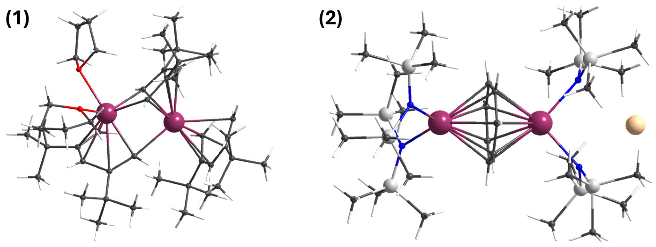
So far, we have consistently neglected compounds (1) and (2) (Figure 7) from our analysis. This is because the coupling constants calculated for these significantly deviate from all other calculations. The fitted exchange coupling constant for (1) is 0.302 cm−1; the best performing four functionals yield values between 0.698 cm−1 and 0.790 cm−1, which is larger than the experimental value. In both cases, the calculated values are too ferromagnetic. For compound (2), the calculated sign of the interaction is wrong, as a value between 0.086 cm−1 and 0.396 cm−1 is calculated, in contrast to the fitted value of −0.096 cm−1. Carbocyclic bridged Gd(III) ions are well known to show significantly stronger exchange interactions compared to other bridges, as seen for the ferromagnetic coupling of compound (1). Most examples feature strong antiferromagnetic interactions, such as in compounds bridged via tetraanion benzene, [29] cycloheptatrienyl as in compound (2), and cyclooctatetraene [122]. Very strong exchange could be realized using tetraanion biphenyl bridges (−0.642 cm−1 and −0.664 cm−1) [123] and another tetraanion benzene bridge with a record value larger than −2.9 cm−1 [124,125]. In contrast, a pyrrolyl-half sandwich compound shows a coupling constant of −0.03 cm−1 [126].
DFT calculations on most of these compounds suggest different reasons for the strong interactions. Either spin polarization of the ligand [122], Gd(III)-ligand interactions with significant covalent contributions [123], or considerable ligand to metal charge transfer characteristics in the ground state [51] are used to rationalize these observations. However, in all cases, the strong interaction of the bridging ligand with both paramagnetic centers is the origin of these strong magnetic couplings. This means that spin localization on the metal centers is of utmost importance for a satisfactory description of the ground state coupling. Spin delocalization is a general problem of pure DFT functionals, whereas HF tends to over-localize spins. Therefore, the result of BS calculations will be subject to the precise amount of HF exchange. This may be even more so the case in (1) and (2) compared to the other molecules in this testbed, as suggested by our analysis of various proportions of HF-exchange (Table S48). Furthermore, when going to more covalent bonds, BS-DFT was recently shown to work less well [127].
In this study, we have tested NBO charges and atomic orbital populations to compare compounds (1) and (2) to the other benchmark molecules. These are chosen as both parameters are commonly used to indicate charge transfer behavior or are used to argue for certain coupling mechanisms. Table S56 contains NBO charges and populations of the 6s and 5d orbitals calculated with the cam-b3lyp functional for all compounds. Here, an approximate 4f75dn6s1-n occupation is calculated for all molecules. While there are 7 electrons in singly occupied orbitals, the eighth electron stems from delocalized electron density in the entire molecule. No relationship between either characteristic and the coupling constant (or the error thereof) can be observed, indicating that NBO charges and populations are, in fact, poor descriptors for the interpretation of the computational results.
Spin densities for compounds (1)(4) are shown exemplarily in Figures S11–S13. While a small spin polarization can be observed for compound (1), only a small amount of beta spin density can be observed for the other molecules. This indicates that the spin-density as an observable may be a good indicator to distinguish between coupling pathways involving spin-polarization and those that do not.
Overlaps of corresponding spin orbitals significantly differing from 1 are provided in Table S57. It becomes apparent that (1) and (2) feature more and more overlapping magnetic orbitals in the broken symmetry state compared to all other tested compounds. This may explain to some extent the qualitatively different behavior.
However, it can be concluded that BS-DFT performs significantly more unreliably for Gd-dimers bridged via carboanions.

8. Results and Discussion IV: Application Example: Gd4-Clusters

For complex spin-systems containing several Gd(III) ions, fitting procedures of effective Spin-Hamiltonians can involve many free parameters compared to rather featureless magnetic data. Thus, deriving these parameters from quantum chemical calculations can give meaningful insight into the individual coupling mechanisms.
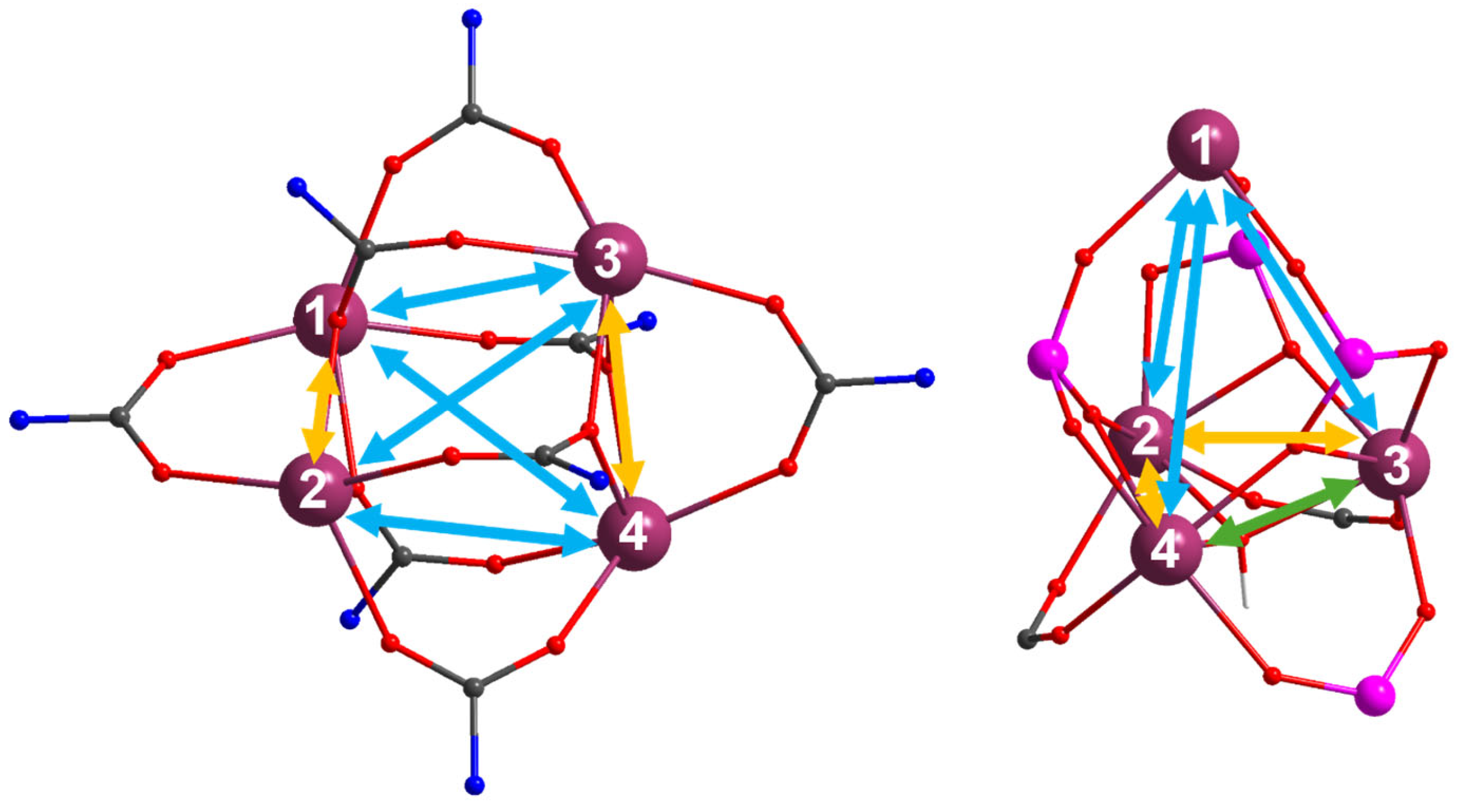
To test the applicability of the proposed methods for more complex spin systems, we have selected two Gd4 clusters with different symmetries. Compound (28) [Gd4(O2CNiPr2)12] is a carbamate bridged Gd4-cluster with C2 symmetry. It contains two different types of bridges: Four carbamate molecules coordinate in a 1κO; 2:3κ2O′-motif where one oxygen bridges between Gd1 and Gd2 (or Gd3 and Gd4) while the other oxygen coordinates to one of Gd3 or Gd4 (or Gd1 or Gd2, respectively). Two further carbamate ligands form syn,syn 1κO; 2κO′-bridges between either Gd1 and Gd3 or Gd2 and Gd4 [128].
Compound (29) [pyH]4[Gd43-OH)(O3PtBu)3(HO3PtBu)(O2CtBu)2(NO3)6 contains a tetranuclear phosphonate core in which the triangular base of three Gd(III) ions is bridged via a central μ3-OH group. The pairs of adjacent Gd(III) in this triangular base are additionally bridged by a chelating-bridging 1:2κ2O; 1κO′ phosphonate linkage and either a 1κO; 2κO′ -carboxylate or a 1κO; 2κO′ -phosphonate bridge. Three phosphonate ions also bridge between two ions in the base and Gd1 in the apical position [129]. Figure 8 illustrates the bridging modes in the cores of the two structures; the full molecules are depicted in Figures S14 and S15. The Gd-Gd distances in compound (28) are 3.882 Å between Gd1-Gd2 and Gd3-Gd4, respectively, significantly shorter than the distances between Gd1-Gd3 and Gd2-Gd4 (4.650 Å) and between Gd1-Gd4 and Gd2-Gd3 (5.033 Å). Similarly, for compound (29), the distances between the apical Gd1 and the other Gd(III) ions are between 5.544 Å and 5.604 Å, which is much longer than the pairs of basal Gd(III), for which the corresponding distances are between 3.809 Å and 3.863 Å.
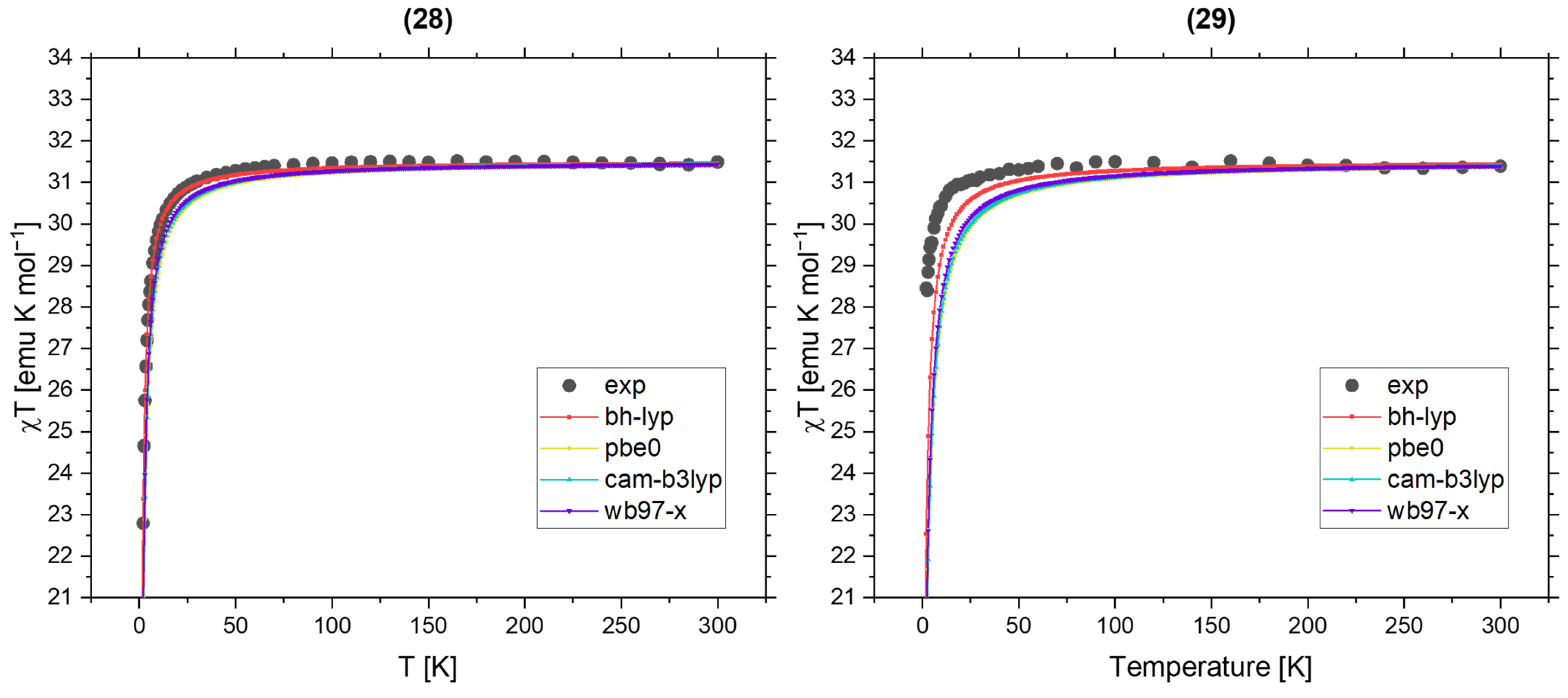
Following the same workflow as described before and using the four functionals we have identified as most suitable, we calculated the exchange coupling constants for both molecules for all six pair interactions. The two Gd(III) ions, which are not of interest for a given calculation, are replaced by diamagnetic Y(III). The resulting coupling constants for the bh-lyp functional are summarized in Table 3. The results for the other functionals are summarized in the SI, Tables S58 and S59. The symmetry of compound (28) is reflected in the calculated coupling constants, meaning that the interaction between Gd1-Gd2 and Gd3-Gd4 is the same. Furthermore, the calculations suggest that only these couplings between ions with short Gd-Gd distances are significant and not the slightly longer contacts Gd1-Gd3 and Gd2-Gd4. Using these coupling constants, the experimental susceptibility (Figure 9 and Figure S16) and magnetization (Figures S17 and S18) can be reproduced excellently (experimental scaled to the theoretical room temperature values). This agreement suggests that this coupling scheme is plausible and the molecule does indeed act as two essentially uncoupled Gd(III) dimers, which is in contrast to the originally proposed model where a second non-zero coupling constant between Gd1-Gd3 and Gd2-Gd4 was necessary to fit the experimental data. Considering the small coupling constants, the re-scaling of the experimental data is equivalent to fitting an anomalous g-factor unequal but close to 2. Consequently, there are no free parameters in the simulations.
The results for compound (29) suggest that Gd1 is essentially uncoupled from the triangular base. Furthermore, the coupling via the carboxylate ligands (Gd2-Gd3 and Gd2-Gd4) is approximately twice as strong as the coupling via the protonated phosphonate (Gd3-Gd4). However, the simulations of the susceptibility and magnetization indicate that DFT is overestimating the real coupling, which leads to a less optimal agreement between simulation and experiment. bh-lyp predicts lower coupling constants than the other three functionals, yet still overestimates the coupling.
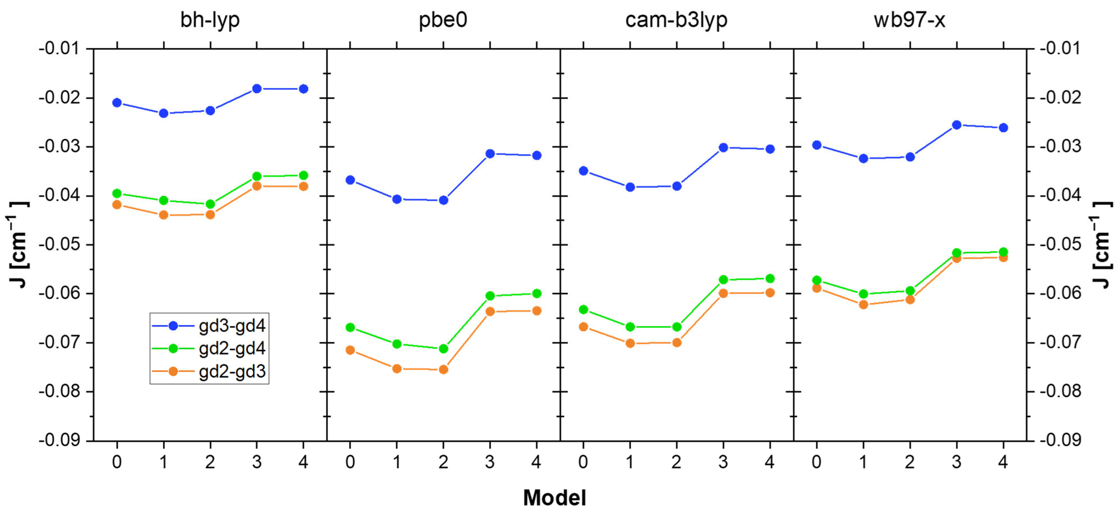
The computational model for compound (29) has a charge of −1 and therefore contains three pyridinium cations, which are hydrogen-bonded to the central molecule. Considering the suboptimal agreement between simulation and experiment, we were wondering whether a reason for this discrepancy is related to the chosen model molecule. Thus, we investigated four truncated versions of the same cluster using the same methods. Pictures of the truncated molecules are displayed in Figure S19. The first truncation is to remove the [Gd(NO3)3] moiety of compound (29). Truncation 2 is to remove all pyridinium cations, changing the charge of the molecule to −4. The third model is to add three protons to the dangling coordination sites of the three phosphonate groups where Gd1 was coordinated. Here, the H-positions are re-optimized with the same method as the original structure. The last truncation is to replace all iso-butyl groups with methyl groups, reducing the size of the model cluster considerably. Again, H-positions are re-optimized.
The results for the four functionals and the 5 models (including the untruncated model as model 0) are summarized in Figure 10. Couplings including Gd1 are excluded as this ion is removed in the first truncation. The values are collected in Table S60. The differences between the various models are collectively below 0.01 cm−1. However, changes that influence the electronic structure immediately around the Gd-ions have a larger influence than those changing the outer sphere. This explains why the coupling constants become more ferromagnetic from model 2 to model 3, whereas almost no change can be observed when replacing the iso-butyl groups with methyl groups. Furthermore, none of the models change the coupling constants significantly enough to achieve a truly good fit to the experiment. We thus conclude that the quality of the calculation using the full model 0 cannot be improved by truncation. The accuracy is, however, within the aforementioned error bars proposed in the benchmark.

9. Conclusions

In conclusion, we report an extensive benchmark study to investigate the dependency of Gd(III)-Gd(III) exchange coupling constants on various computational parameters, aiming to establish best practices. It is shown that DFT is a viable method to predict exchange coupling constants for a wide range of Gd-dimers with an accuracy of <0.02 cm−1. The following best practices can be suggested:
  • A triple-ζ basis is necessary to describe the central ion and the surrounding ligands satisfactorily.
  • Scalar relativistic effects should be taken into account explicitly. Similar results were obtained using DKH2, DKH4, and X2C. Neglecting scalar relativistic effects or using ECPs leads to inaccuracies in the same order of magnitude as those induced by the DFT functional.
  • We tested 25 different DFT functionals and would like to discourage the use of LDAs, GGAs, and meta-GGAs since they did not yield sufficiently accurate values. Considering a balance between computational cost and accuracy, we suggest using four functionals in parallel: the hybrid functionals bh-lyp and pbe0, as well as the range-separated functionals cam-b3lyp and ωb97-x. Using these four functionals will give a range of values close to the experimental value. Other hybrid functionals such as tpss0, b3-lyp, b97, and bhandhlyp, as well as the range-separated ωb97, and the local hybrid tmhf perform similarly well.
  • We have shown that truncating the model complex is a feasible way to reduce the computational cost significantly. For example, replacing isobutyl groups with methyl groups has resulted in no significant change in the calculated coupling constants for all tested functionals. However, changes to atoms with a significant influence on the coordination site of the ligand may have an influence on the calculated coupling constant.
Furthermore, we have shown that an ideal amount of exact HF-exchange is close to 35%. During this comparative study, we could also indicate that within a given range of Gd(III)-Gd(III) distances, there is a roughly linear dependency of the distance on the coupling constant, while we find no such influence of the bridging angle in our structurally diverse testbed. However, this may be the case for compounds with similar bridges.
This relationship (and the DFT functionals in general) does not apply to Gd(III) dimers bridged via organometallic ligands. These compounds cannot be computed as reliably with DFT, significantly overestimating the coupling constants.
Finally, we have shown that our best practice methods can be used to model more complex spin systems, such as Gd4-clusters, with good accuracy, and even in cases where DFT does not give excellent agreements with experimental data, it can still provide valuable starting parameters for the Spin-Hamiltonian-based fitting functions.

Supplementary Materials

The following supporting information can be downloaded at: https://www.mdpi.com/article/10.3390/magnetochemistry12060067/s1. Figure S1. Structures (1)(12) of the testbed. Gd ions are dark purple, H white, Si silver, C dark gray, O red, N blue, S yellow, Cl green, F gold, K tan, Li light blue, Zn sea green. Hydrogen bonds are indicated as segmented orange bonds. Figure S2. Structures (13)(24) of the testbed. Gd ions are dark purple, H white, Si silver, C dark gray, O red, N blue, P pink, S yellow, Cl green, F gold, K tan, Li light blue, Zn sea green. Hydrogen bonds are indicated as segmented orange bonds. Figure S3. Structures (25)(27) of the testbed. Gd ions are dark purple, H white, Si silver, C dark gray, O red, N blue, S yellow, Cl green, F gold, K tan, Li light blue, Zn sea green. Hydrogen bonds are indicated as segmented orange bonds. Figure S4. Energies of HS-single point calculation of compound (10) using the b3-lyp functional with 100% exact exchange. This is a common trend for single point calculations failing at the high spin calculation. The calculation is initiated with 14 electrons at the two Gd(III) centers using an extended Hückel guess. First, the energy converges cleanly to the correct ground state. Usually, using our options and setup this took between 80–120 iterations to reach the defined convergence criteria. In this case however, the SCF algorithm then finds a lower minimum indicated by the clear step above 200 iterations. The final spin density of this calculation is shown in Figure S5. Figure S5. This picture shows the spin density (isodensity = 0.005) of the converged calculation of Figure S4. Blue indicates α, red indicates β spin density. Clearly, formerly occupied orbitals at the ligand split and formed this complicated and non-physical density. Therefore, no meaningful results can be extracted from this data. Figure S6. Calculated exchange coupling constants against their experimental values using the functionals pbe0 (top left), cam-b3lyp (top right), ωb97-x (bottom left) and an average using the 4 suggested functionals (bh-lyp in addition to the ones shown here). The colors indicate the bridging ion, the diagonal line indicates experimental accuracy. The horizontal and vertical lines indicate 0. Consequently, points in the top left and bottom right quarter of each graph predict the wrong coupling sign. The light blue highlighted area indicates the mean absolute error for each functional. Figure S7. Linear regression for the four best performing functionals as well as their average. Figure S8. Calculated coupling constants for the functionals pbeo (top left), cam-b3lyp (top right), ωb97-x (bottom left) and the experimental values (bottom right) against the Gd(III)-Gd(III) distance. The area of correlation between 3.7 Å and 4.2 Å is highlighted in green. For a easier comparison we sorted the molecules by their bridging motifs. The bridging atoms corresponds to the color, for O-bridged molecules, these are sorted into alcoholate bridged (OR), carboxylate bridged (OAc) and other bridges (O*). If two different bridges are present in one compound, the respective symbols are superimposed. Figure S9. Calculated coupling constants for the functionals pbeo (top left), cam-b3lyp (top right), ωb97-x (bottom left) and the experimental values (bottom right) against the smallest Gd(III)-L-Gd(III) angle in °. No correlation can be observed for any of the data sets. For a easier comparison we sorted the molecules by their bridging motifs. The bridging atoms corresponds to the color, for O-bridged molecules, these are sorted into alcoholate bridged (OR), carboxylate bridged (OAc) and other bridges (O*). If two different bridges are present in one compound, the respective symbols are superimposed. Figure S10. Correlation between the Gd-Gd bridging angle and the coupling constant for molecules bridged via two alcoholates in the testbed. Figure S11. Spin densities for compounds (1) and (2) calculated with cam-b3lyp at an isovalue of 0.005. Blue indicates alpha and red beta spin. Figure S12. Spin densities for compounds (3) and (4) calculated with cam-b3lyp at an isovalue of 0.005. Blue indicates alpha and red beta spin. Figure S13. Spin density for compounds (8) calculated with m06 at an isovalue of 0.005. Blue indicates alpha and red beta spin. The visually larger spin polarization may be the cause for the large error in this calculation. Figure S14. structure of compound (28). Purple atoms are Gd, red O, blue N, gray C and white H. Figure S15. Structure of compound (29). Purple atoms are Gd, pink P, red O, blue N, gray C and white H. Hydrogen bonds are indicated by segmented, orange bonds. Figure S16. Simulated Susceptibility for compound (28) using the four suggested functionals but only considering one unique coupling constant between Gd1-Gd2 and Gd3-Gd4. Figure S17. Simulated Magnetization versus Temperature plot using the four suggested functionals for compound (28). The low temperature high field value is scaled exactly to the theoretical of 5 which is equal to fitting an anomalous g-factor. Figure S18. Simulated Magnetization versus Temperature plot using the four suggested functionals for compound (29). The low temperature high field value is scaled exactly to the theoretical of 5 which is equal to fitting an anomalous g-factor. Figure S19. Truncated structures of compound (29). Purple atoms are Gd, pink P, red O, blue N, gray C and white H. Hydrogen bonds are indicated by segmented, orange bonds. For truncation 1 (top left), the [Gd1(NO3)3] moiety was removed. For truncation 2 (top right) the pyridinium ions were removed changing the total charge of the compound to -4. For truncation 3 (bottom left), hydrogen atoms were added to the empty coordination sites of the three phosphonate sites. For truncation 4 (bottom right) all isobutyl-groups were replaced with methyl groups. Table S1. Summary of energies associated to the four Kramers Doublets of each Gd(III) ions ground state of the testbed molecules in cm−1. The last column is the calculated isotropic g-value for a Pseudospin S = 7/2. Table S2. Extended Steven Operators for each ion in structures (1) and (2). Table S3. Extended Steven Operators for each ion in structures (3) and (4). Table S4. Extended Steven Operators for each ion in structures (5) and (6). Table S5. Extended Steven Operators for each ion in structures (7) and (8). Table S6. Extended Steven Operators for each ion in structures (9) and (10). Table S7. Extended Steven Operators for each ion in structures (11) and (12). Table S8. Extended Steven Operators for each ion in structures (13) and (14). Table S9. Extended Steven Operators for each ion in structures (15) and (16). Table S10. Extended Steven Operators for each ion in structures (17) and (18). Table S11. Extended Steven Operators for each ion in structures (19) and (20). Table S12. Extended Steven Operators for each ion in structures (21) and (22). Table S13. Extended Steven Operators for each ion in structures (23) and (24). Table S14. Extended Steven Operators for each ion in structures (25) and (26). Table S15. Extended Steven Operators for each ion in structure (27). Table S16. Reference data from Papers as well as g-factors and coupling constants J fitted with a Bleaney-Bowers equation. a: difference to fit presumably because of faulty Hamiltonian definition. b: using original data; c: keeping g fixed to fit the high temperature value as 1.99; d: excluding data after anomalous jump. *: this model is used as reference in this benchmark. Table S17. Reference data from Papers as well as g-factors and coupling constants J fitted with the Lines model in PHI. a: difference to fit presumably because of faulty Hamiltonian definition. b: using original data; c: keeping g fixed to fit the high temperature value as 1.99; d: excluding data after anomalous jump. *: this model is used as reference in this benchmark. Table S18. Reference data from Papers as well as g-factors and coupling constants J fitted with the Lines model in PHI using crystal field parameters from CASOCI. a: difference to fit presumably because of faulty Hamiltonian definition. b: using original data; c: keeping g fixed to fit the high temperature value as 1.99; d: excluding data after anomalous jump. *: this model is used as reference in this benchmark. Table S19. Exchange coupling constants in cm−1 for compounds (1)(5) using different functions. The names XXX-YYY-ZZZ indicate which level of basis was used for Gd(III), ligand atoms and hydrogen atoms respectively. Calculations that did not converge or did not finish within a reasonable time are indicated with a “-”. Table S20. Exchange coupling constants in cm−1 for compounds (6)(10) using different functions. The names XXX-YYY-ZZZ indicate which level of basis was used for Gd(III), ligand atoms and hydrogen atoms respectively. Calculations that did not converge or did not finish within a reasonable time are indicated with a “-”. Table S21. Exchange coupling constants in cm−1 for compounds (11)(15) using different functions. The names XXX-YYY-ZZZ indicate which level of basis was used for Gd(III), ligand atoms and hydrogen atoms respectively. Calculations that did not converge or did not finish within a reasonable time are indicated with a “-”. Table S22. Exchange coupling constants in cm−1 for compounds (16)(20) using different functions. The names XXX-YYY-ZZZ indicate which level of basis was used for Gd(III), ligand atoms and hydrogen atoms respectively. Calculations that did not converge or did not finish within a reasonable time are indicated with a “-”. Table S23. Exchange coupling constants in cm−1 for compounds (21)(25) using different functions. The names XXX-YYY-ZZZ indicate which level of basis was used for Gd(III), ligand atoms and hydrogen atoms respectively. Calculations that did not converge or did not finish within a reasonable time are indicated with a “-”. Table S24. Exchange coupling constants in cm−1 for compounds (26) and (27) using different functions. The names XXX-YYY-ZZZ indicate which level of basis was used for Gd(III), ligand atoms and hydrogen atoms respectively. Calculations that did not converge or did not finish within a reasonable time are indicated with a “-”. Table S25. Mean absolute errors (MAE) and Standard deviations (std dev) for each basis set combination with respect to the largest basis used, QZVPP-TZVPP-TZVP. As the errors are significantly larger for molecules (1) and (2) compared to the remaining testbed, MAE and std dev excluding these are given as well. Table S26. Exchange coupling constants calculated for different levels of treatment for scalar relativistic effects in cm−1. Table S27. Exchange coupling constants calculated for grid sizes in cm−1. Table S28. Exchange coupling constants calculated with x2c-TZVPall+DD basis set in cm−1. Table S29. Exchange coupling constants calculated with different with different functionals for compounds (1)(5) in cm−1. Table S30. Exchange coupling constants calculated with different with different functionals for compounds (6)(10) in cm−1. Table S31. Exchange coupling constants calculated with different with different functionals for compounds (11)(15) in cm−1. Table S32. Exchange coupling constants calculated with different with different functionals for compounds (16)(20) in cm−1. Table S33. Exchange coupling constants calculated with different with different functionals for compounds (21)(25) in cm−1. Table S34. Exchange coupling constants calculated with different with different functionals for compounds (26), (27) in cm−1. Table S35. High Spin ⟨S2⟩ expectation values calculated with different with different functionals for compounds (1)(5) in cm−1. Table S36. High Spin ⟨S2⟩ expectation values calculated with different with different functionals for compounds (6)(10) in cm−1. Table S37. High Spin ⟨S2⟩ expectation values calculated with different with different functionals for compounds (11)(15) in cm−1. Table S38. High Spin ⟨S2⟩ expectation values calculated with different with different functionals for compounds (16)(20) in cm−1. Table S39. High Spin ⟨S2⟩ expectation values calculated with different with different functionals for compounds (21)(25) in cm−1. Table S40. High Spin ⟨S2⟩ expectation values calculated with different with different functionals for compounds (26), (27) in cm−1. Table S41. Low Spin ⟨S2⟩ expectation values calculated with different with different functionals for compounds (1)(5) in cm−1. Table S42. Low Spin ⟨S2⟩ expectation values calculated with different with different functionals for compounds (6)(10) in cm−1. Table S43. Low Spin ⟨S2⟩ expectation values calculated with different with different functionals for compounds (11)(15) in cm−1. Table S44. Low Spin ⟨S2⟩ expectation values calculated with different with different functionals for compounds (16)(20) in cm−1. Table S45. Low Spin ⟨S2⟩ expectation values calculated with different with different functionals for compounds (21)(25) in cm−1. Table S46. Low Spin ⟨S2⟩ expectation values calculated with different with different functionals for compounds (26), (27) in cm−1. Table S47. Mean absolute Deviation (MAD), mean deviation (MD), Max absolute deviation (MaxAD) and Root mean square deviations (RMSD) for all functionals in cm−1. The calculation for molecule (8) has resulted in a deviation of 1.8 cm−1 with respect to the experimental data. Hence, this calculation is excluded (the values including it are given in brackets). Also, molecules (1) and (2) are excluded from this data. Table S48. Exchange coupling constants calculated for molecules (1)(5) using the b3-lyp functional with a custom amount of exact exchange (first column) in cm−1. Table S49. Exchange coupling constants calculated for molecules (6)(10) using the b3-lyp functional with a custom amount of exact exchange (first column) in cm−1. Table S50. Exchange coupling constants calculated for molecules (11)(15) using the b3-lyp functional with a custom amount of exact exchange (first column) in cm−1. Table S51. Exchange coupling constants calculated for molecules (16)(20) using the b3-lyp functional with a custom amount of exact exchange (first column) in cm−1. Table S52. Exchange coupling constants calculated for molecules (21)(25) using the b3-lyp functional with a custom amount of exact exchange (first column) in cm−1. Table S53. Exchange coupling constants calculated for molecules (26) and (27) as well as the average and standard deviation of the Errors with respect to the experimental values excluding molecules (1) and (2) using the b3-lyp functional with a custom amount of exact exchange (first column) in cm−1. Table S54. If a calculation did not converge after 300 iterations this is a very good indication it will not converge to the correct ground state. However, as the calculation is not converged yet, ⟨S2HS may not significantly deviate from 56 yet. In Figure S4, this is in the approximate area between 140 and 200 iterations. However, already at this point the density reorganization takes place which would feature an increasing change in the density. Therefore, even if the calculation is not fully converged, either, ⟨S2HS deviating from 56 or increasing density differences from iteration 299 to 300 can be taken as strong indications that the calculation has become unstable. This is shown below for all calculations for which no Jex could be reported in the HF test. (a) Converged after 287 iterations (b) HS state converged, but instability occurred in the BS state (c) Error in calculation script. Table S55. Compounds for which the MaxAD values are associated in Figure 3. All largest deviations to the experiment across the 25 functionals are due to five compounds. Table S56. NBO-charges and occupations of valence orbitals for the high spin states of the testbed molecules. Table S57. Overlap of corresponding spin orbitals <0.999 for all compounds using the cam-b3lyp functional. Table S58. Calculated exchange coupling constants for compound (28) using the functionals pbe0, cam-b3lyp and ωb97-x in cm−1. Table S59. Calculated exchange coupling constants for compound (29) using the functionals pbe0, cam-b3lyp and ωb97-x in cm−1. Table S60. Calculated exchange coupling constants for truncated models of compound (29) using the functionals bh-lyp, pbe0, cam-b3lyp and ωb97-x in cm−1.

Author Contributions

C.F.P.; conceptualization, formal analysis, investigation, writing—original draft preparation, J.B.; conceptualization, data curation, writing—review & editing, C.E.A.; conceptualization, writing—review & editing, K.F.; conceptualization, funding acquisition, investigation, supervision, writing—review & editing. All authors have read and agreed to the published version of the manuscript.

Funding

This research was funded by DFG CRC 1573 “4f for Future”, the Helmholtz Association POF MSE, and the Landesgraduiertenförderung Baden-Württemberg.

Data Availability Statement

The data are contained within the article and supporting information. xyz-files to reproduce the calculations have been uploaded to KITOpen and can be accessed using the following https://doi.org/10.35097/mudjr5vgtzrwzuj9 (accessed on 6 June 2026).

Acknowledgments

We would like to thank the DFG CRC 1573 “4f for Future”, the Helmholtz Association POF MSE, and the Landesgraduiertenförderung Baden-Württemberg for the funding of this research. We also like to thank those who have kindly contributed experimental data for this benchmark.

Conflicts of Interest

The authors declare no conflicts of interest.

References

  1. Zhu, Z.; Paul, S.; Zhao, C.; Wu, J.; Ying, X.; Ungur, L.; Wernsdorfer, W.; Meyer, F.; Tang, J. Record Quantum Tunneling Time in an Air-Stable Exchange-Bias Dysprosium Macrocycle. J. Am. Chem. Soc. 2024, 146, 18899–18904. [Google Scholar] [CrossRef] [Scilit] [PubMed]
  2. Yi, X.; Bernot, K.; Cador, O.; Luzon, J.; Calvez, G.; Daiguebonne, C.; Guillou, O. Influence of Ferromagnetic Connection of Ising-Type Dy(III)-Based Single Ion Magnets on Their Magnetic Slow Relaxation. Dalton Trans. 2013, 42, 6728–6731. [Google Scholar] [CrossRef] [Scilit]
  3. Moreno-Pineda, E.; Chilton, N.F.; Marx, R.; Dörfel, M.; Sells, D.O.; Neugebauer, P.; Jiang, S.-D.; Collison, D.; van Slageren, J.; McInnes, E.J.L.; et al. Direct Measurement of Dysprosium(III)···dysprosium(III) Interactions in a Single-Molecule Magnet. Nat. Commun. 2014, 5, 5243. [Google Scholar] [CrossRef] [Scilit]
  4. Pfleger, R.F.; Briganti, M.; Bonde, N.; Ollivier, J.; Braun, J.; Bergfeldt, T.; Piligkos, S.; Ruppert, T.; Anson, C.E.; Perfetti, M.; et al. Dinuclear Dysprosium Compounds: The Importance of Rigid Bridges. Chem. Eur. J. 2025, 31, e202403002. [Google Scholar] [CrossRef] [Scilit]
  5. Tziotzi, T.G.; Gracia, D.; Dalgarno, S.J.; Schnack, J.; Evangelisti, M.; Brechin, E.K.; Milios, C.J. A {Gd12Na6} Molecular Quadruple-Wheel with a Record Magnetocaloric Effect at Low Magnetic Fields and Temperatures. J. Am. Chem. Soc. 2023, 145, 7743–7747. [Google Scholar] [CrossRef] [Scilit] [PubMed]
  6. Braun, J.; Seufert, D.; Anson, C.E.; Tang, J.; Powell, A.K. An Effectively Uncoupled Gd8 Cluster Formed through Fixation of Atmospheric CO2 Showing Excellent Magnetocaloric Properties. Int. J. Mol. Sci. 2023, 25, 264. [Google Scholar] [CrossRef] [Scilit]
  7. Sharples, J.W.; Zheng, Y.-Z.; Tuna, F.; McInnes, E.J.L.; Collison, D. Lanthanide Discs Chill Well and Relax Slowly. Chem. Commun. 2011, 47, 7650. [Google Scholar] [CrossRef] [Scilit] [PubMed]
  8. Tishin, A.M.; Spichkin, Y.I. The Magnetocaloric Effect and Its Applications, 1st ed.; CRC Press: Boca Raton, FL, USA, 2003. [Google Scholar]
  9. Zheng, Y.-Z.; Zhou, G.-J.; Zheng, Z.; Winpenny, R.E.P. Molecule-Based Magnetic Coolers. Chem. Soc. Rev. 2014, 43, 1462–1475. [Google Scholar] [CrossRef] [Scilit]
  10. Sharples, J.W.; Collison, D.; McInnes, E.J.L.; Schnack, J.; Palacios, E.; Evangelisti, M. Quantum Signatures of a Molecular Nanomagnet in Direct Magnetocaloric Measurements. Nat. Commun. 2014, 5, 5321. [Google Scholar] [CrossRef] [Scilit]
  11. Tang, J.; Hewitt, I.; Madhu, N.T.; Chastanet, G.; Wernsdorfer, W.; Anson, C.E.; Benelli, C.; Sessoli, R.; Powell, A.K. Dysprosium Triangles Showing Single-Molecule Magnet Behavior of Thermally Excited Spin States. Angew. Chem. Int. Ed. 2006, 45, 1729–1733. [Google Scholar] [CrossRef] [Scilit]
  12. Chibotaru, L.F.; Ungur, L.; Soncini, A. The Origin of Nonmagnetic Kramers Doublets in the Ground State of Dysprosium Triangles: Evidence for a Toroidal Magnetic Moment. Angew. Chem. Int. Ed. 2008, 47, 4126–4129. [Google Scholar] [CrossRef] [Scilit]
  13. Hymas, K.; Soncini, A. The Role of Magnetic Dipole—Dipole Coupling in Quantum Single-Molecule Toroics. Magnetochemistry 2022, 8, 58. [Google Scholar] [CrossRef] [Scilit]
  14. Dolai, M.; Moreno-Pineda, E.; Wernsdorfer, W.; Ali, M.; Ghosh, A. Exchange-Bias Quantum Tunneling of the Magnetization in a Dysprosium Dimer. J. Phys. Chem. A 2021, 125, 8230–8237. [Google Scholar] [CrossRef] [Scilit] [PubMed]
  15. Wernsdorfer, W.; Aliaga-Alcalde, N.; Hendrickson, D.N.; Christou, G. Exchange-Biased Quantum Tunnelling in a Supramolecular Dimer of Single-Molecule Magnets. Nature 2002, 416, 406–409. [Google Scholar] [CrossRef] [Scilit] [PubMed]
  16. Guo, Y.-N.; Xu, G.-F.; Wernsdorfer, W.; Ungur, L.; Guo, Y.; Tang, J.; Zhang, H.-J.; Chibotaru, L.F.; Powell, A.K. Strong Axiality and Ising Exchange Interaction Suppress Zero-Field Tunneling of Magnetization of an Asymmetric Dy2 Single-Molecule Magnet. J. Am. Chem. Soc. 2011, 133, 11948–11951. [Google Scholar] [CrossRef] [Scilit] [PubMed]
  17. Dunstan, M.A.; Mole, R.A.; Boskovic, C. Inelastic Neutron Scattering of Lanthanoid Complexes and Single-Molecule Magnets. Eur. J. Inorg. Chem. 2019, 2019, 1090–1105. [Google Scholar] [CrossRef] [Scilit]
  18. Kettles, F.J.; Milway, V.A.; Tuna, F.; Valiente, R.; Thomas, L.H.; Wernsdorfer, W.; Ochsenbein, S.T.; Murrie, M. Exchange Interactions at the Origin of Slow Relaxation of the Magnetization in {TbCu3} and {DyCu3} Single-Molecule Magnets. Inorg. Chem. 2014, 53, 8970–8978. [Google Scholar] [CrossRef] [Scilit]
  19. Loewenhaupt, M.; Tils, P.; Buschow, K.H.J.; Eccleston, R.S. Exchange Interactions in GdFe Compounds Studied by Inelastic Neutron Scattering. J. Magn. Magn. Mater. 1996, 152, 10–16. [Google Scholar] [CrossRef] [Scilit]
  20. Chibotaru, L.F. Theoretical Understanding of Anisotropy in Molecular Nanomagnets. In Molecular Nanomagnets and Related Phenomena; Gao, S., Ed.; Structure and Bonding; Springer: Berlin/Heidelberg, Germany, 2014; Volume 164, pp. 185–229. [Google Scholar]
  21. Schray, D.; Westerbeck, D.; Braun, J.; Lan, Y.; Gómez-Coca, S.; Wernsdorfer, W.; Ruiz, E.; Anson, C.E.; Schnack, J.; Powell, A.K. Fe–Gd Ferromagnetic Cyclic Coordination Cluster [FeIII4 GdIII4 (teaH)8 (N3)8 (H2O)] with Magnetic Anisotropy—Theory and Experiment. Inorg. Chem. 2023, 62, 6642–6648. [Google Scholar] [CrossRef] [Scilit]
  22. Essajai, R.; Ennassiri, N.; Balli, M.; Zidane, M.; Salmani, E.; Mounkachi, O.; Rouchdi, M.; Abbassi, A.; Ez-Zahraouy, H.; Mzerd, A.; et al. Revisiting the Magnetic and Magnetocaloric Properties of Bulk Gadolinium: A Combined DFT and Monte Carlo Simulations. Phys. Scr. 2020, 96, 015808. [Google Scholar] [CrossRef] [Scilit]
  23. Rajaraman, G.; Totti, F.; Bencini, A.; Caneschi, A.; Sessoli, R.; Gatteschi, D. Density Functional Studies on the Exchange Interaction of a Dinuclear Gd(III)-Cu(II) Complex: Method Assessment, Magnetic Coupling Mechanism and Magneto-Structural Correlations. Dalton Trans. 2009, 17, 3153–3161. [Google Scholar] [CrossRef] [Scilit]
  24. Rajeshkumar, T.; Singh, S.K.; Rajaraman, G. A Computational Perspective on Magnetic Coupling, Magneto-Structural Correlations and Magneto-Caloric Effect of a Ferromagnetically Coupled {GdIII–GdIII} Pair. Polyhedron 2013, 52, 1299–1305. [Google Scholar] [CrossRef] [Scilit]
  25. Langley, S.K.; Wielechowski, D.P.; Vieru, V.; Chilton, N.F.; Moubaraki, B.; Abrahams, B.F.; Chibotaru, L.F.; Murray, K.S. A {Cr(III)2Dy(III)2} Single-Molecule Magnet: Enhancing the Blocking Temperature through 3d Magnetic Exchange. Angew. Chem. Int. Ed. 2013, 52, 12014–12019. [Google Scholar] [CrossRef] [Scilit] [PubMed]
  26. Ungur, L.; van den Heuvel, W.; Chibotaru, L.F. Ab Initio Investigation of the Non-Collinear Magnetic Structure and the Lowest Magnetic Excitations in Dysprosium Triangles. New J. Chem. 2009, 33, 1224–1230. [Google Scholar] [CrossRef] [Scilit]
  27. Noodleman, L. Valence Bond Description of Antiferromagnetic Coupling in Transition Metal Dimers. J. Chem. Phys. 1981, 74, 5737–5743. [Google Scholar] [CrossRef] [Scilit]
  28. Onishi, T.; Yamaki, D.; Yamaguchi, K.; Takano, Y. Theoretical Calculations of Effective Exchange Integrals by Spin Projected and Unprojected Broken-Symmetry Methods. I. Cluster Models of K2NiF4-Type Solids. J. Chem. Phys. 2003, 118, 9747–9761. [Google Scholar] [CrossRef] [Scilit]
  29. Jin, P.-B.; Luo, Q.-C.; Gransbury, G.K.; Winpenny, R.E.P.; Mills, D.P.; Zheng, Y.-Z. Rare Earth Benzene Tetraanion-Bridged Amidinate Complexes. Chem. Sci. 2025, 16, 1907–1924. [Google Scholar] [CrossRef] [Scilit]
  30. Roy, L.E.; Hughbanks, T. Magnetic Coupling in Dinuclear Gd Complexes. J. Am. Chem. Soc. 2006, 128, 568–575. [Google Scholar] [CrossRef] [Scilit]
  31. Costa, R.; Reta, D.; Moreira, I.D.P.R.; Illas, F. Post-B3LYP Functionals Do Not Improve the Description of Magnetic Coupling in Cu(II) Dinuclear Complexes. J. Phys. Chem. A 2018, 122, 3423–3432. [Google Scholar] [CrossRef] [Scilit]
  32. Phillips, J.J.; Peralta, J.E. Magnetic Exchange Couplings from Semilocal Functionals Evaluated Nonself-Consistently on Hybrid Densities: Insights on Relative Importance of Exchange, Correlation, and Delocalization. J. Chem. Theory Comput. 2012, 8, 3147–3158. [Google Scholar] [CrossRef] [Scilit]
  33. Moreira, I.D.P.R.; Costa, R.; Filatov, M.; Illas, F. Restricted Ensemble-Referenced Kohn−Sham versus Broken Symmetry Approaches in Density Functional Theory: Magnetic Coupling in Cu Binuclear Complexes. J. Chem. Theory Comput. 2007, 3, 764–774. [Google Scholar] [CrossRef] [Scilit]
  34. Valero, R.; Costa, R.; De P.R. Moreira, I.; Truhlar, D.G.; Illas, F. Performance of the M06 Family of Exchange-Correlation Functionals for Predicting Magnetic Coupling in Organic and Inorganic Molecules. J. Chem. Phys. 2008, 128, 114103. [Google Scholar] [CrossRef] [Scilit]
  35. David, G.; Wennmohs, F.; Neese, F.; Ferré, N. Chemical Tuning of Magnetic Exchange Couplings Using Broken-Symmetry Density Functional Theory. Inorg. Chem. 2018, 57, 12769–12776. [Google Scholar] [CrossRef] [Scilit]
  36. Rivero, P.; Moreira, I.D.P.R.; Illas, F.; Scuseria, G.E. Reliability of Range-Separated Hybrid Functionals for Describing Magnetic Coupling in Molecular Systems. J. Chem. Phys. 2008, 129, 184110. [Google Scholar] [CrossRef] [Scilit]
  37. Singh, G.; Gamboa, S.; Orio, M.; Pantazis, D.A.; Roemelt, M. Magnetic Exchange Coupling in Cu Dimers Studied with Modern Multireference Methods and Broken-Symmetry Coupled Cluster Theory. Theor. Chem. Acc. 2021, 140, 139. [Google Scholar] [CrossRef] [Scilit]
  38. López, C.; Costa, R.; Illas, F.; De Graaf, C.; Turnbull, M.M.; Landee, C.P.; Espinosa, E.; Mata, I.; Molins, E. Magneto-Structural Correlations in Binuclear Copper(II) Compounds Bridged by a Ferrocenecarboxylato(–1) and an Hydroxo- or Methoxo-Ligands. Dalton Trans. 2005, 13, 2322–2330. [Google Scholar] [CrossRef] [Scilit]
  39. Paulovič, J.; Cimpoesu, F.; Ferbinteanu, M.; Hirao, K. Mechanism of Ferromagnetic Coupling in Copper(II)-Gadolinium(III) Complexes. J. Am. Chem. Soc. 2004, 126, 3321–3331. [Google Scholar] [CrossRef] [Scilit] [PubMed]
  40. Yan, F.; Chen, Z. Magnetic Coupling Constants and Spin Density Maps for Heterobinuclear Complexes GdCu(OTf)3(Bdmap)2(H2O)·THF, [Gd(C4H7ON)4(H2O)3][Fe(CN)6]·2H2O, and [Gd(C4H7ON)4 (H2O)3][Cr(CN)6]·2H2O: A Density Functional Study. J. Phys. Chem. A 2000, 104, 6295–6300. [Google Scholar] [CrossRef] [Scilit]
  41. Rajeshkumar, T.; Jose, R.; Remya, P.R.; Rajaraman, G. Theoretical Studies on Trinuclear {MnIII2 GdIII} and Tetranuclear {MnIII2 GdIII2} Clusters: Magnetic Exchange, Mechanism of Magnetic Coupling, Magnetocaloric Effect, and Magneto–Structural Correlations. Inorg. Chem. 2019, 58, 11927–11940. [Google Scholar] [CrossRef] [Scilit] [PubMed]
  42. Singh, S.K.; Pedersen, K.S.; Sigrist, M.; Thuesen, C.A.; Schau-Magnussen, M.; Mutka, H.; Piligkos, S.; Weihe, H.; Rajaraman, G.; Bendix, J. Angular Dependence of the Exchange Interaction in Fluoride-Bridged GdIII–CrIII Complexes. Chem. Commun. 2013, 49, 5583. [Google Scholar] [CrossRef] [Scilit]
  43. Singh, S.K.; Rajaraman, G. Decisive Interactions That Determine Ferro/Antiferromagnetic Coupling in {3d–4f} Pairs: A Case Study on Dinuclear {V(IV)–Gd(III)} Complexes. Dalton Trans. 2013, 42, 3623. [Google Scholar] [CrossRef] [Scilit]
  44. Singh, S.K.; Tibrewal, N.K.; Rajaraman, G. Density Functional Studies on Dinuclear {NiIIGdIII} and Trinuclear {NiIIGdIIINiII} Complexes: Magnetic Exchange and Magneto-Structural Maps. Dalton Trans. 2011, 40, 10897. [Google Scholar] [CrossRef] [Scilit]
  45. Gupta, T.; Rajeshkumar, T.; Rajaraman, G. Magnetic Exchange in {GdIII–Radical} Complexes: Method Assessment, Mechanism of Coupling and Magneto-Structural Correlations. Phys. Chem. Chem. Phys. 2014, 16, 14568–14577. [Google Scholar] [CrossRef] [Scilit]
  46. Cirera, J.; Ruiz, E. Exchange Coupling in CuIIGdIII Dinuclear Complexes: A Theoretical Perspective. Comptes Rendus Chim. 2008, 11, 1227–1234. [Google Scholar] [CrossRef] [Scilit]
  47. Anderson, P.W. Antiferromagnetism. Theory of Superexchange Interaction. Phys. Rev. 1950, 79, 350–356. [Google Scholar] [CrossRef] [Scilit]
  48. Goodenough, J.B. Theory of the Role of Covalence in the Perovskite-Type Manganites [La, M(II)] MnO3. Phys. Rev. 1955, 100, 564–573. [Google Scholar] [CrossRef] [Scilit]
  49. Kanamori, J. Superexchange Interaction and Symmetry Properties of Electron Orbitals. J. Phys. Chem. Solids 1959, 10, 87–98. [Google Scholar] [CrossRef] [Scilit]
  50. Raeder, J.; Reiners, M.; Baumgarten, R.; Münster, K.; Baabe, D.; Freytag, M.; Jones, P.G.; Walter, M.D. Synthesis and Molecular Structure of Pentadienyl Complexes of the Rare-Earth Metals. Dalton Trans. 2018, 47, 14468–14482. [Google Scholar] [CrossRef] [Scilit]
  51. Harriman, K.L.M.; Le Roy, J.J.; Ungur, L.; Holmberg, R.J.; Korobkov, I.; Murugesu, M. Cycloheptatrienyl Trianion: An Elusive Bridge in the Search of Exchange Coupled Dinuclear Organolanthanide Single-Molecule Magnets. Chem. Sci. 2017, 8, 231–240. [Google Scholar] [CrossRef] [Scilit]
  52. Tuna, F.; Smith, C.A.; Bodensteiner, M.; Ungur, L.; Chibotaru, L.F.; McInnes, E.J.L.; Winpenny, R.E.P.; Collison, D.; Layfield, R.A. A High Anisotropy Barrier in a Sulfur-Bridged Organodysprosium Single-Molecule Magnet. Angew. Chem. Int. Ed. 2012, 51, 6976–6980. [Google Scholar] [CrossRef] [Scilit]
  53. Lu, Y.-B.; Wu, J.-W.; Zhu, S.-D.; Wang, S.-Q.; Zhang, S.-Y.; Liu, C.-M.; Li, R.; Li, J.; Ai, J.-H.; Xie, Y.-R. 3-Pyridylacetic-Based Lanthanide Complexes Exhibiting Magnetic Entropy Changes, Single-Molecule Magnet, and Fluorescence. ACS Omega 2022, 7, 2604–2612. [Google Scholar] [CrossRef] [Scilit]
  54. Rasamsetty, A.; Mehta, S.; Ansari, K.U.; Kumar, P.; Mondal, A.; Shanmugam, M. Six-Coordinated Dinuclear Lanthanide(III) Amide Complexes: Investigation of Magnetization Relaxation Dynamics and Their Electronic Structures. Dalton Trans. 2022, 51, 63–68. [Google Scholar] [CrossRef] [Scilit]
  55. Han, T.; Ding, Y.-S.; Li, Z.-H.; Yu, K.-X.; Zhai, Y.-Q.; Chilton, N.F.; Zheng, Y.-Z. A Dichlorido-Bridged Dinuclear Dy(III) Single-Molecule Magnet with an Effective Energy Barrier Larger than 600 K. Chem. Commun. 2019, 55, 7930–7933. [Google Scholar] [CrossRef] [Scilit]
  56. Jung, J.; Benner, F.; Herbst-Irmer, R.; Demir, S.; Stalke, D. Slow Magnetic Relaxation in Mono- and Bimetallic Lanthanide Tetraimido-Sulfate S(N t Bu)42− Complexes. Chem. Eur. J. 2021, 27, 12310–12319. [Google Scholar] [CrossRef] [Scilit]
  57. Layfield, R.A.; Bashall, A.; McPartlin, M.; Rawson, J.M.; Wright, D.S. A Structural and Magnetic Study of Organolanthanide(III) Amides. Dalton Trans. 2006, 13, 1660–1666. [Google Scholar] [CrossRef] [Scilit]
  58. Mukherjee, S.; Lu, J.; Velmurugan, G.; Singh, S.; Rajaraman, G.; Tang, J.; Ghosh, S.K. Influence of Tuned Linker Functionality on Modulation of Magnetic Properties and Relaxation Dynamics in a Family of Six Isotypic Ln2 (Ln = Dy and Gd) Complexes. Inorg. Chem. 2016, 55, 11283–11298. [Google Scholar] [CrossRef] [Scilit]
  59. Liu, C.; Hao, X.; Zhang, D. CO2-fixation into Carbonate Anions for the Construction of 3d-4f Cluster Complexes with Salen-type Schiff Base Ligands: From Molecular Magnetic Refrigerants to Luminescent Single-molecule Magnets. Appl. Oganomet. Chem. 2020, 34, e5893. [Google Scholar] [CrossRef] [Scilit]
  60. Kalita, P.; Goura, J.; Manuel Herrera Martínez, J.; Colacio, E.; Chandrasekhar, V. Homodinuclear {LnIII2} (LnIII = GdIII, TbIII, HoIII, and DyIII) Complexes: Field-Induced SMM Behavior of the DyIII and TbIII Analogues. Eur. J. Inorg. Chem. 2019, 2019, 212–220. [Google Scholar] [CrossRef] [Scilit]
  61. Liu, Z.; Huang, X.; Chen, Z.; Liu, D.; Zou, H.; Liang, F. Exploring the Functional Relation of Magnetic Density and Magnetocaloric Effect Based on a Dinuclear System. Appl. Oganomet. Chem. 2021, 35, e6325. [Google Scholar] [CrossRef] [Scilit]
  62. John, D.; Urland, W. Crystal Structure and Magnetic Behaviour of the New Gadolinium Carboxylates Gd2 (ClF2CCOO)6 (Hypy)2, Gd2 (F3CCOO)6 (Hypy)2, Gd2 (F2HCCOO)6 (Hypy)2 and Gd2 (Cl2HCCOO)6 (H2O)2 (Hypy)2. Eur. J. Inorg. Chem. 2006, 2006, 3503–3509. [Google Scholar] [CrossRef] [Scilit]
  63. Wang, H.; Liu, C.; Liu, T.; Zeng, S.; Cao, W.; Ma, Q.; Duan, C.; Dou, J.; Jiang, J. Mixed (Phthalocyaninato)(Schiff-Base) Di-Dysprosium Sandwich Complexes. Effect of Magnetic Coupling on the SMM Behavior. Dalton Trans. 2013, 42, 15355–15360. [Google Scholar] [CrossRef] [Scilit] [PubMed]
  64. Machata, M.; Herchel, R.; Nemec, I.; Trávníček, Z. Crystal Structures and Magnetic Properties of Two Series of Phenoxo-O Bridged Dinuclear Ln2 (Ln = Gd, Tb, Dy) Complexes. Dalton Trans. 2017, 46, 16294–16305. [Google Scholar] [CrossRef] [Scilit] [PubMed]
  65. Zhou, M.; Wu, L.-H.; Wu, X.-Y.; Yao, S.-L.; Zheng, T.-F.; Xie, X.; Liu, S.-J. Two Dinuclear GdIII Clusters Based on Isobutyric Acid and Nicotinic Acid with Large Magnetocaloric Effects. J. Mol. Struct. 2021, 1227, 129689. [Google Scholar] [CrossRef] [Scilit]
  66. Zhang, H.; Lin, S.-Y.; Xue, S.; Wang, C.; Tang, J. Acetato-Bridged Dinuclear Lanthanide Complexes with Single Molecule Magnet Behaviour for the Dy2 Species. Dalton Trans. 2014, 43, 6262–6268. [Google Scholar] [CrossRef] [Scilit]
  67. Meng, Z.-S.; Guo, F.-S.; Liu, J.-L.; Leng, J.-D.; Tong, M.-L. Heterometallic Cubane-like {M2Ln2} (M = Ni, Zn; Ln =, Gd, Dy) and {Ni2Y2} Aggregates. Synthesis, Structures and Magnetic Properties. Dalton Trans. 2012, 41, 2320–2329. [Google Scholar] [CrossRef] [Scilit]
  68. Chu, X.-Y.; Wang, W.-M.; Nie, Y.-Y.; Cui, J.-Z.; Gao, H.-L. Regulating the Luminescent and Magnetic Properties of Rare-Earth Complexes with β-Diketonate Coligands. New J. Chem. 2018, 42, 11417–11429. [Google Scholar] [CrossRef] [Scilit]
  69. Mylonas-Margaritis, I.; Mayans, J.; Sakellakou, S.-M.; Raptopoulou, C.P.; Psycharis, V.; Escuer, A.; Perlepes, S.P. Using the Singly Deprotonated Triethanolamine to Prepare Dinuclear Lanthanide(III) Complexes: Synthesis, Structural Characterization and Magnetic Studies. Magnetochemistry 2017, 3, 5. [Google Scholar] [CrossRef] [Scilit]
  70. Bao, S.; Ma, L.; Wang, Y.; Fang, L.; Zhu, C.; Li, Y.; Zheng, L. Anion-Directed Self-Assembly of Lanthanide–Notp Compounds and Their Fluorescence, Magnetic, and Catalytic Properties. Chem. Eur. J. 2007, 13, 2333–2343. [Google Scholar] [CrossRef] [Scilit]
  71. Ehama, K.; Ohmichi, Y.; Sakamoto, S.; Fujinami, T.; Matsumoto, N.; Mochida, N.; Ishida, T.; Sunatsuki, Y.; Tsuchimoto, M.; Re, N. Synthesis, Structure, Luminescent, and Magnetic Properties of Carbonato-Bridged ZnII2 LnIII2 Complexes [(μ4-CO3)2 {ZnII LnLnIII (NO3)}2] (LnIII = GdIII, TbIII, DyIII.; L1 = N,N′-Bis(3-Methoxy-2-Oxybenzylidene)-1,3-Propanediaminato, L2 = N,N′-Bis(3-Ethoxy-2-Oxybenzylidene)-1,3-Propanediaminato). Inorg. Chem. 2013, 52, 12828–12841. [Google Scholar] [CrossRef] [Scilit]
  72. Xiong, J.; Ding, H.-Y.; Meng, Y.-S.; Gao, C.; Zhang, X.-J.; Meng, Z.-S.; Zhang, Y.-Q.; Shi, W.; Wang, B.-W.; Gao, S. Hydroxide-Bridged Five-Coordinate DyIII Single-Molecule Magnet Exhibiting the Record Thermal Relaxation Barrier of Magnetization among Lanthanide-Only Dimers. Chem. Sci. 2017, 8, 1288–1294. [Google Scholar] [CrossRef] [Scilit]
  73. Ullmann, S.; Hahn, P.; Blömer, L.; Mehnert, A.; Laube, C.; Abel, B.; Kersting, B. Dinuclear Lanthanide Complexes Supported by a Hybrid Salicylaldiminato/Calix [4]Arene-Ligand: Synthesis, Structure, and Magnetic and Luminescence Properties of (HNEt3)[Ln2 (HL)(L)] (Ln = SmIII, EuIII, GdIII, TbIII). Dalton Trans. 2019, 48, 3893–3905. [Google Scholar] [CrossRef] [Scilit] [PubMed]
  74. Hutchings, A.-J.; Habib, F.; Holmberg, R.J.; Korobkov, I.; Murugesu, M. Structural Rearrangement Through Lanthanide Contraction in Dinuclear Complexes. Inorg. Chem. 2014, 53, 2102–2112. [Google Scholar] [CrossRef] [Scilit]
  75. Weigend, F.; Ahlrichs, R. Balanced Basis Sets of Split Valence, Triple Zeta Valence and Quadruple Zeta Valence Quality for H to Rn: Design and Assessment of Accuracy. Phys. Chem. Chem. Phys. 2005, 7, 3297–3305. [Google Scholar] [CrossRef] [Scilit] [PubMed]
  76. Becke, A.D. A New Mixing of Hartree–Fock and Local Density-functional Theories. J. Chem. Phys. 1993, 98, 1372–1377. [Google Scholar] [CrossRef] [Scilit]
  77. Becke, A.D. Density-Functional Exchange-Energy Approximation with Correct Asymptotic Behavior. Phys. Rev. A 1988, 38, 3098–3100. [Google Scholar] [CrossRef] [Scilit]
  78. Becke, A.D. Density-Functional Thermochemistry. III. The Role of Exact Exchange. J. Chem. Phys. 1993, 98, 5648–5652. [Google Scholar] [CrossRef] [Scilit]
  79. Lee, C.; Yang, W.; Parr, R.G. Development of the Colle-Salvetti Correlation-Energy Formula into a Functional of the Electron Density. Phys. Rev. B 1988, 37, 785–789. [Google Scholar] [CrossRef] [Scilit]
  80. Eichkorn, K.; Weigend, F.; Treutler, O.; Ahlrichs, R. Auxiliary Basis Sets for Main Row Atoms and Transition Metals and Their Use to Approximate Coulomb Potentials. Theor. Chim. Acta 1997, 97, 119–124. [Google Scholar] [CrossRef] [Scilit]
  81. Weigend, F. A Fully Direct RI-HF Algorithm: Implementation, Optimised Auxiliary Basis Sets, Demonstration of Accuracy and Efficiency. Phys. Chem. Chem. Phys. 2002, 4, 4285–4291. [Google Scholar] [CrossRef] [Scilit]
  82. Caldeweyher, E.; Ehlert, S.; Hansen, A.; Neugebauer, H.; Spicher, S.; Bannwarth, C.; Grimme, S. A Generally Applicable Atomic-Charge Dependent London Dispersion Correction. J. Chem. Phys. 2019, 150, 154122. [Google Scholar] [CrossRef] [Scilit]
  83. Caldeweyher, E.; Bannwarth, C.; Grimme, S. Extension of the D3 Dispersion Coefficient Model. J. Chem. Phys. 2017, 147, 034112. [Google Scholar] [CrossRef] [Scilit] [PubMed]
  84. A Development of University of Karlsruhe and Forschungszentrum Karlsruhe GmbH, TURBOMOLE V7.7 2022; University of Karlsruhe: Karlsruhe, Germany; Forschungszentrum Karlsruhe GmbH: Karlsruhe, Germany, 1989–2007, TURBOMOLE GmbH, Since 2007. Available online: https://www.turbomole.org (accessed on 6 June 2026).
  85. Balasubramani, S.G.; Chen, G.P.; Coriani, S.; Diedenhofen, M.; Frank, M.S.; Franzke, Y.J.; Furche, F.; Grotjahn, R.; Harding, M.E.; Hättig, C.; et al. TURBOMOLE: Modular Program Suite for Ab Initio Quantum-Chemical and Condensed-Matter Simulations. J. Chem. Phys. 2020, 152, 184107. [Google Scholar] [CrossRef] [Scilit] [PubMed]
  86. Pollak, P.; Weigend, F. Segmented Contracted Error-Consistent Basis Sets of Double- and Triple-ζ Valence Quality for One- and Two-Component Relativistic All-Electron Calculations. J. Chem. Theory Comput. 2017, 13, 3696–3705. [Google Scholar] [CrossRef] [Scilit]
  87. Peng, D.; Middendorf, N.; Weigend, F.; Reiher, M. An Efficient Implementation of Two-Component Relativistic Exact-Decoupling Methods for Large Molecules. J. Chem. Phys. 2013, 138, 184105. [Google Scholar] [CrossRef] [Scilit]
  88. van Wüllen, C. Relation between Different Variants of the Generalized Douglas-Kroll Transformation through Sixth Order. J. Chem. Phys. 2004, 120, 7307–7313. [Google Scholar] [CrossRef] [Scilit] [PubMed]
  89. van Wüllen, C.; Michauk, C. Accurate and Efficient Treatment of Two-Electron Contributions in Quasirelativistic High-Order Douglas-Kroll Density-Functional Calculations. J. Chem. Phys. 2005, 123, 204113. [Google Scholar] [CrossRef] [Scilit]
  90. Bodenstein, T.; Heimermann, A.; Fink, K.; van Wüllen, C. Development and Application of a Complete Active Space Spin-Orbit Configuration Interaction Program Designed for Single Molecule Magnets. Chemphyschem 2022, 23, 202100648. [Google Scholar] [CrossRef] [Scilit]
  91. Van Vleck, J.H. The Theory of Electric and Magnetic Susceptibilities; Monographs on Physics; Oxford University Press: Oxford, UK, 1932. [Google Scholar]
  92. Bleaney, B.; Bowers, K.D. Anomalous Paramagnetism of Copper Acetate. Proc. R. Soc. Lond. A 1952, 214, 451–465. [Google Scholar] [CrossRef] [Scilit]
  93. O’Connor, C.J. Magnetochemistry—Advances in Theory and Experimentation. In Progress in Inorganic Chemistry; Lippard, S.J., Ed.; Wiley: Hoboken, NJ, USA, 1982; Volume 29, pp. 203–283. [Google Scholar]
  94. Chilton, N.F.; Anderson, R.P.; Turner, L.D.; Soncini, A.; Murray, K.S. PHI: A Powerful New Program for the Analysis of Anisotropic Monomeric and Exchange-Coupled Polynuclear d- and f-Block Complexes. J. Comput. Chem. 2013, 34, 1164–1175. [Google Scholar] [CrossRef] [Scilit]
  95. Lines, M.E. Orbital Angular Momentum in the Theory of Paramagnetic Clusters. J. Chem. Phys. 1971, 55, 2977–2984. [Google Scholar] [CrossRef] [Scilit]
  96. Palii, A.; Tsukerblat, B.; Clemente-Juan, J.M.; Coronado, E. Magnetic Exchange between Metal Ions with Unquenched Orbital Angular Momenta: Basic Concepts and Relevance to Molecular Magnetism. Int. Rev. Phys. Chem. 2010, 29, 135–230. [Google Scholar] [CrossRef] [Scilit]
  97. Stevens, K.W.H. Matrix Elements and Operator Equivalents Connected with the Magnetic Properties of Rare Earth Ions. Proc. Phys. Soc. A 1952, 65, 209–215. [Google Scholar] [CrossRef] [Scilit]
  98. Bleaney, B.; Stevens, K.W.H. Paramagnetic Resonance. Rep. Prog. Phys. 1953, 16, 108–159. [Google Scholar] [CrossRef] [Scilit]
  99. Franzke, Y.J.; Spiske, L.; Pollak, P.; Weigend, F. Segmented Contracted Error-Consistent Basis Sets of Quadruple-ζ Valence Quality for One- and Two-Component Relativistic All-Electron Calculations. J. Chem. Theory Comput. 2020, 16, 5658–5674. [Google Scholar] [CrossRef] [Scilit]
  100. Slater, J.C. A Simplification of the Hartree-Fock Method. Phys. Rev. 1951, 81, 385–390. [Google Scholar] [CrossRef] [Scilit]
  101. Vosko, S.H.; Wilk, L.; Nusair, M. Accurate Spin-Dependent Electron Liquid Correlation Energies for Local Spin Density Calculations: A Critical Analysis. Can. J. Phys. 1980, 58, 1200–1211. [Google Scholar] [CrossRef] [Scilit]
  102. Perdew, J.P.; Wang, Y. Accurate and Simple Analytic Representation of the Electron-Gas Correlation Energy. Phys. Rev. B 1992, 45, 13244–13249. [Google Scholar] [CrossRef] [Scilit] [PubMed]
  103. Perdew, J.P. Density-Functional Approximation for the Correlation Energy of the Inhomogeneous Electron Gas. Phys. Rev. B 1986, 33, 8822–8824. [Google Scholar] [CrossRef] [Scilit]
  104. Perdew, J.P.; Burke, K.; Ernzerhof, M. Generalized Gradient Approximation Made Simple. Phys. Rev. Lett. 1996, 77, 3865–3868. [Google Scholar] [CrossRef] [Scilit] [PubMed]
  105. Staroverov, V.N.; Scuseria, G.E.; Tao, J.; Perdew, J.P. Comparative Assessment of a New Nonempirical Density Functional: Molecules and Hydrogen-Bonded Complexes. J. Chem. Phys. 2003, 119, 12129–12137. [Google Scholar] [CrossRef] [Scilit]
  106. Tao, J.; Perdew, J.P.; Staroverov, V.N.; Scuseria, G.E. Climbing the Density Functional Ladder: Nonempirical Meta-Generalized Gradient Approximation Designed for Molecules and Solids. Phys. Rev. Lett. 2003, 91, 146401. [Google Scholar] [CrossRef] [Scilit]
  107. Wang, Y.; Jin, X.; Yu, H.S.; Truhlar, D.G.; He, X. Revised M06-L Functional for Improved Accuracy on Chemical Reaction Barrier Heights, Noncovalent Interactions, and Solid-State Physics. Proc. Natl. Acad. Sci. USA 2017, 114, 8487–8492. [Google Scholar] [CrossRef] [Scilit] [PubMed]
  108. Sun, J.; Ruzsinszky, A.; Perdew, J.P. Strongly Constrained and Appropriately Normed Semilocal Density Functional. Phys. Rev. Lett. 2015, 115, 036402. [Google Scholar] [CrossRef] [Scilit]
  109. Becke, A.D. Density-Functional Thermochemistry. V. Systematic Optimization of Exchange-Correlation Functionals. J. Chem. Phys. 1997, 107, 8554–8560. [Google Scholar] [CrossRef] [Scilit]
  110. Grimme, S. Accurate Calculation of the Heats of Formation for Large Main Group Compounds with Spin-Component Scaled MP2 Methods. J. Phys. Chem. A 2005, 109, 3067–3077. [Google Scholar] [CrossRef] [Scilit] [PubMed]
  111. Perdew, J.P.; Ernzerhof, M.; Burke, K. Rationale for Mixing Exact Exchange with Density Functional Approximations. J. Chem. Phys. 1996, 105, 9982–9985. [Google Scholar] [CrossRef] [Scilit]
  112. Adamo, C.; Barone, V. Toward Reliable Density Functional Methods without Adjustable Parameters: The PBE0 Model. J. Chem. Phys. 1999, 110, 6158–6170. [Google Scholar] [CrossRef] [Scilit]
  113. Yanai, T.; Tew, D.P.; Handy, N.C. A New Hybrid Exchange–Correlation Functional Using the Coulomb-Attenuating Method (CAM-B3LYP). Chem. Phys. Lett. 2004, 393, 51–57. [Google Scholar] [CrossRef] [Scilit]
  114. Chai, J.-D.; Head-Gordon, M. Systematic Optimization of Long-Range Corrected Hybrid Density Functionals. J. Chem. Phys. 2008, 128, 084106. [Google Scholar] [CrossRef] [Scilit]
  115. Holzer, C.; Franzke, Y.J. A Local Hybrid Exchange Functional Approximation from First Principles. J. Chem. Phys. 2022, 157, 034108. [Google Scholar] [CrossRef] [Scilit]
  116. Holzer, C.; Franzke, Y.J. A General and Transferable Local Hybrid Functional for Electronic Structure Theory and Many-Fermion Approaches. J. Chem. Theory Comput. 2025, 21, 202–217. [Google Scholar] [CrossRef] [Scilit]
  117. Bahmann, H.; Rodenberg, A.; Arbuznikov, A.V.; Kaupp, M. A Thermochemically Competitive Local Hybrid Functional without Gradient Corrections. J. Chem. Phys. 2007, 126, 011103. [Google Scholar] [CrossRef] [Scilit]
  118. Fürst, S.; Kaupp, M.; Wodyński, A. Range-Separated Local Hybrid Functionals with Small Fractional-Charge and Fractional-Spin Errors: Escaping the Zero-Sum Game of DFT Functionals. J. Chem. Theory Comput. 2023, 19, 8639–8653. [Google Scholar] [CrossRef] [Scilit]
  119. Moreira, I.D.P.R.; Illas, F.; Martin, R.L. Effect of Fock Exchange on the Electronic Structure and Magnetic Coupling in NiO. Phys. Rev. B 2002, 65, 155102. [Google Scholar] [CrossRef] [Scilit]
  120. Spearman, C. The Proof and Measurement of Association between Two Things. Am. J. Psychol. 1904, 15, 72. [Google Scholar] [CrossRef] [Scilit]
  121. Pearson, K. Note on Regression and Inheritance in the Case of Two Parents. Proc. R. Soc. Lond. 1895, 58, 240–242. [Google Scholar] [CrossRef] [Scilit]
  122. Le Roy, J.J.; Jeletic, M.; Gorelsky, S.I.; Korobkov, I.; Ungur, L.; Chibotaru, L.F.; Murugesu, M. An Organometallic Building Block Approach To Produce a Multidecker 4f Single-Molecule Magnet. J. Am. Chem. Soc. 2013, 135, 3502–3510. [Google Scholar] [CrossRef] [Scilit]
  123. Huang, W.; Le Roy, J.J.; Khan, S.I.; Ungur, L.; Murugesu, M.; Diaconescu, P.L. Tetraanionic Biphenyl Lanthanide Complexes as Single-Molecule Magnets. Inorg. Chem. 2015, 54, 2374–2382. [Google Scholar] [CrossRef] [Scilit]
  124. McClain, K.R.; Vincent, A.H.; Rajabi, A.; Ngo, D.X.; Meihaus, K.R.; Furche, F.; Harvey, B.G.; Long, J.R. Linear Inverse Sandwich Complexes of Tetraanionic Benzene Stabilized by Covalent δ-Bonding with Late Lanthanides. J. Am. Chem. Soc. 2024, 146, 32708–32716. [Google Scholar] [CrossRef] [Scilit]
  125. Liu, M.; Chen, Y.-C.; Mondal, A.; Wang, H.; Tong, M.-L.; Layfield, R.A.; Guo, F.-S. η6-Benzene Tetra-Anion Complexes of Early and Late Rare-Earth Metals. J. Am. Chem. Soc. 2025, 147, 11359–11367. [Google Scholar] [CrossRef] [Scilit]
  126. She, Y.; Lu, Y.; Jia, C.; Li, Y.; Zhang, Y.-Q.; Yao, J. Organolanthanide η1- and η5-Pyrrolyl Half-Sandwich Compounds: Synthesis, Structures, and Magnetic Properties. New J. Chem. 2023, 47, 15650–15657. [Google Scholar] [CrossRef] [Scilit]
  127. Iwahara, N.; Huang, Z.; Mansikkamäki, A.; Chibotaru, L.F. Breakdown of Broken-Symmetry Approach to Exchange Interaction. J. Chem. Phys. 2025, 162, 164701. [Google Scholar] [CrossRef] [Scilit]
  128. Moreno-Pineda, E.; Lan, Y.; Fuhr, O.; Wernsdorfer, W.; Ruben, M. Exchange-Bias Quantum Tunnelling in a CO2-Based Dy4-Single Molecule Magnet. Chem. Sci. 2017, 8, 1178–1185. [Google Scholar] [CrossRef] [Scilit]
  129. Zangana, K.H.; Pineda, E.M.; Winpenny, R.E.P. Tetrametallic Lanthanide(III) Phosphonate Cages: Synthetic, Structural and Magnetic Studies. Dalton Trans. 2014, 43, 17101–17107. [Google Scholar] [CrossRef] [Scilit]
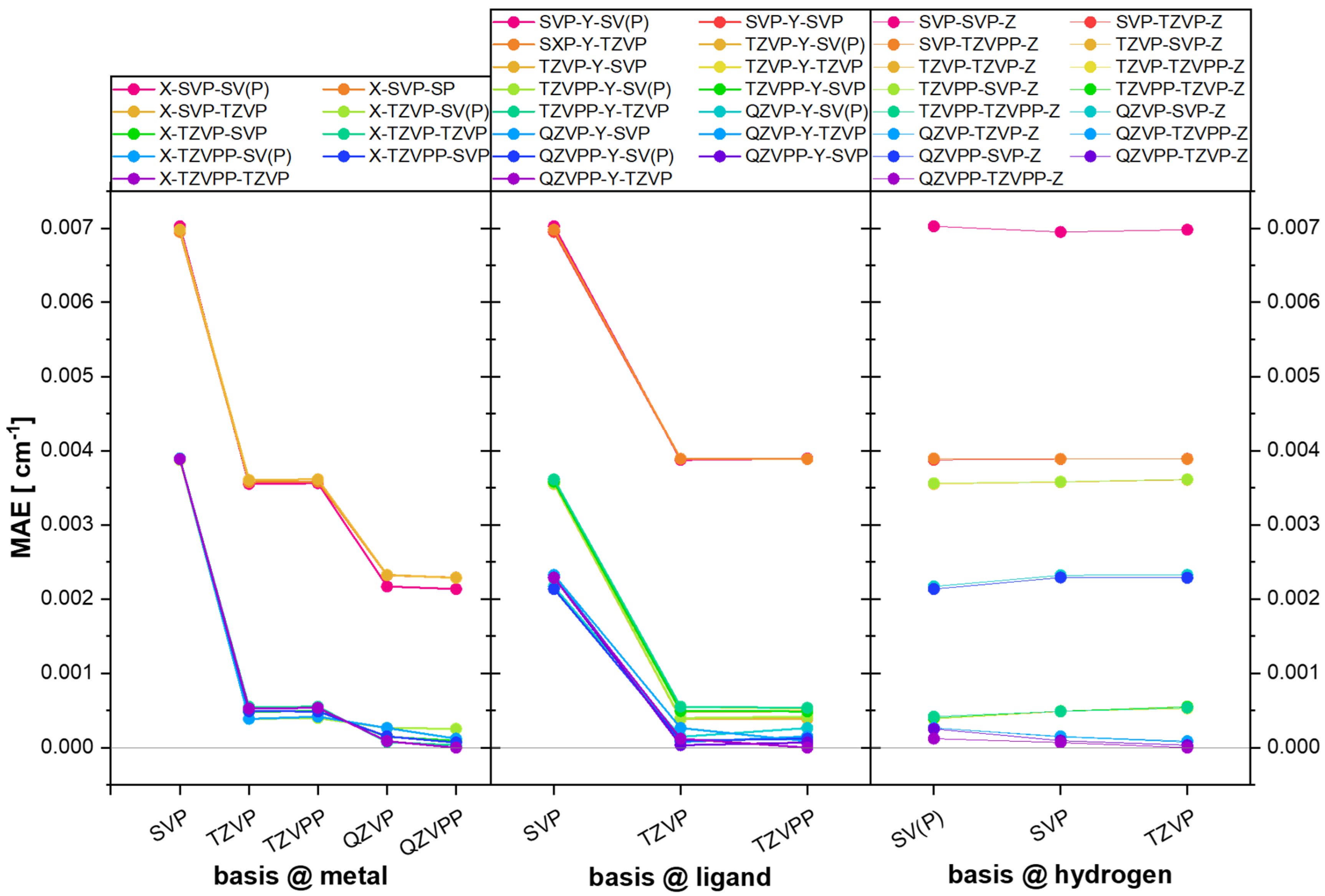
Figure 1. Mean Absolute Errors (MAE) of different basis set combinations. (left) Keeping ligand and hydrogen basis fixed while varying the basis for the metal. (middle) Keeping metal and hydrogen basis fixed and varying the basis used to describe the ligand. (right) Keeping metal and ligand basis sets fixed while changing the basis for hydrogen atoms. All basis sets used are from the segmented contracted all-electron X2C-basis set family.
Magnetochemistry 12 00067 g001
Figure 2. Mean Absolute Errors (MAE) with respect to X2C for different treatments of scalar relativistic effects. While no treatment and ECPs lead to larger errors, DKH2, DKH4, and X2C give the same result within reasonable accuracy.
Magnetochemistry 12 00067 g002
Figure 3. Mean absolute deviation (MAD), mean deviation (MD), and maximum absolute deviation (Max AD) for all functionals investigated. Root mean square deviations (RMSD) are shown in Table S47. Molecules (1) and (2) are excluded from this data, and (8) is excluded from the calculation for the m06 functional.
Magnetochemistry 12 00067 g003
Figure 4. Absolute Error between the exchange coupling constant calculated using a certain amount of HF-exchange vs. the amount of HF-exchange for the testbed molecules excluding (1) and (2). The blue line is the average (MAE), and errors are calculated as standard deviations.
Magnetochemistry 12 00067 g004
Figure 5. Calculated exchange coupling constants calculated using the suggested bh-lyp functional against experimental values. The diagonal line indicates an exact match, the light blue area indicates the mean absolute deviation for bh-lyp. The vertical and horizontal lines indicate zero.
Magnetochemistry 12 00067 g005
Figure 6. (left) Calculated coupling constants using the bh-lyp functional against Gd(III)-Gd(III) distances in Å. The area of correlation between 3.7 Å and 4.2 Å is highlighted in green. Compounds (3), (5), (6), and (26) are outside the highlighted area, indicating a different relaxation pathway. (right) Calculated coupling constants using the bh-lyp functional against Gd(III)-L-Gd(III) angles. No correlation can be observed.
Magnetochemistry 12 00067 g006
Figure 7. Molecular structures of compounds (1) and (2). Gd ions are dark purple, H white, Si silver, C dark gray, O red, N blue, K tan.
Magnetochemistry 12 00067 g007
Figure 8. Core structures of molecules (28) (left) and (29) (right). Only Gd atoms are numbered to compare to the interactions discussed. Blue arrows indicate negligible coupling according to the calculations. Orange and green arrows indicate significant coupling according to our calculations.
Magnetochemistry 12 00067 g008
Figure 9. Simulated susceptibility using the BS-exchange coupling constants for compounds (28) and (29). The experimental susceptibility is scaled to the high temperature value of 31.52 emu K mol−1 for four uncoupled Gd(III) ions. This procedure is equivalent to fitting an anomalous g-factor which is very close to 2.
Magnetochemistry 12 00067 g009
Figure 10. Calculated exchange coupling constants for the four suggested functionals and the five model complexes for compound (29). For pictures of the structures, see Figure S18.
Magnetochemistry 12 00067 g010
Table 1. References, formulae, bridging atom, Gd-Gd distance, and Gd-L-Gd angles for all structures investigated in this benchmark.
Nr. Formula Bridging
Atoms
Gd-Gd Dist. (Å) Gd-L-Gd
Angles (°)
Coupling Ref.
(1)[(pdl’)(pdl’−1H)(pdl’−2H)Gd2(thf)2]C3.24681.0–82.3FM[50]
(2)[KGd2(C7H7)(N(SiMe3)2)4]C4.087102.9–103.5AF[51]
(3)[{Cp’2Gd(μ-SSiPh3)}2]S4.316101.5AF[52]
(4)[Gd2(3-PAA)2(μ-Cl)2(phen)4](ClO4)2Cl, O3.90689.7AF[53]
(5)[Gd2(μ-Cl)2Cl4Li2(L)2(THF)6]Cl4.376102.6AF[54]
(6)[Gd(Cy2N)2(μ-Cl)(THF)]2Cl4.303102.6AF[55]
(7)[{(THF)2Li(NtBu)2S(tBuN)2GdCl2}2•ClLi(thf)2]Cl3.83586.0/89.4AF[56]
(8)[Cp2Gd{2-NH-4,6-Me2pm}]2N3.81198.3/100.2AF[57]
(9)[Gd2(L3)2(L’)2(MeOH)2]O3.859110.8AF[58]
(10)[Zn2Gd23-CO3)2(Lb)2(NO3)2]•2MeOHO4.070116.8FM[59]
(11)[NHEt3]2[Gd2(μ-NO3)2(NO3)2(HL)2]O3.761107.9AF[60]
(12)[Gd2(HL)2(NO3)4]•2MeCNO3.855108.4AF[61]
(13)[Gd2(F2HCCOO)6(hypy)2]O3.880106.8AF[62]
(14)[Gd2(ClF2CCOO)6(hypy)2]O3.866106.5AF[62]
(15)[Gd2(Cl2HCCOO)6(H2O)2(hypy)2]O4.051107.6AF[62]
(16)[Zn2Gd2L2Cl2(OAc)4(MeOH)2]O4.081112.0FM[63]
(17)[Gd2(3m-L4)2(L2)2(DMF)2]O3.815106.3AF[64]
(18)[Gd2(iba)6(bipy)2]O3.948106.4AF[65]
(19)[Gd2L2(OAc)4(MeOH)2]•2MeOHO4.099112.0AF[66]
(20)[Zn2Gd2(μ-OH)2(L)2(OAc)5(EtOH)(H2O)] •2EtOH•1.5H2OO3.791105.6/104.5AF[67]
(21)[Gd2(dbm)2L2(MeOH)2]•nMeOHO3.987113.0AF[68]
(22)[Gd2(NO3)4(teaH2)2]O3.719109.3AF[69]
(23)[Gd{C9N3H20(PO3H)2(PO3)}(NO3)(H2O)]2•8H2OO4.028110.1AF[70]
(24)[(μ4-CO3)2{ZnL1Gd(NO3)}2]•acetone•2H2OO4.045116.5FM[71]
(25)[Gd(μ-OH)(DBP)2(THF)2]2O3.748110.5AF[72]
(26)(HNEt3)[Gd2(HL)(L)]O3.896107.9AF[73]
(27)[Gd2(Hhmb)3(NCS)3]•2MeOH•pyO3.599101.1/95.7/100.8AF[74]
Table 2. Summary of fitted J-values (-2 J formalism, see Equation (1)) of all testbed molecules. These values are used as a reference for later comparisons.
BridgeJ (cm−1) BridgeJ (cm−1) BridgeJ (cm−1)
(1)C0.302 (6)(10)O0.024 (0)(19)O−0.006 (0)
(2)C−0.096 (1)(11)O−0.097 (1)(20)O−0.029 (0)
(3)S−0.098 (1)(12)O−0.058 (0)(21)O−0.032 (0)
(4)Cl/O−0.020 (1)(13)O−0.062 (1)(22)O−0.143 (1)
(5)Cl−0.075 (2)(14)O−0.022 (1)(23)O−0.011 (0)
(6)Cl−0.033 (1)(15)O−0.014 (0)(24)O0.039 (1)
(7)Cl−0.036 (1)(16)O0.020 (0)(25)O−0.115 (0)
(8)O−0.069 (1)(17)O−0.072 (1)(26)O−0.066 (0)
(9)O−0.036 (1)(18)O−0.021 (1)(27)O−0.022 (0)
Table 3. Calculated exchange coupling constants for compounds (28) and (29) in cm−1 using the bh-lyp functional compared to the values reported in Refs. [128,129].
Interaction(28) DFT/Exp. (Ref [128])(29) DFT/Exp. (Ref [129])
Gd1-Gd2−0.035/−0.0580.001/0.00
Gd1-Gd30.002/0.0120.001/0.00
Gd1-Gd4−0.001/0.0000.001/0.00
Gd2-Gd3−0.001/0.000−0.042/−0.01
Gd2-Gd40.000/0.012−0.040/−0.01
Gd3-Gd4−0.035/−0.058−0.021/−0.01
Disclaimer/Publisher’s Note: The statements, opinions and data contained in all publications are solely those of the individual author(s) and contributor(s) and not of MDPI and/or the editor(s). MDPI and/or the editor(s) disclaim responsibility for any injury to people or property resulting from any ideas, methods, instructions or products referred to in the content.