Article

A Temperature-Corrected High-Frequency Non-Sinusoidal Excitation Core Loss Prediction Model

1
School of Electrical and Energy Power Engineering, Yangzhou University, Yangzhou 225000, China
2
School of Mechanical Engineering, Yangzhou University, Yangzhou 225000, China
*
Author to whom correspondence should be addressed.
Magnetochemistry 2026, 12(1), 6; https://doi.org/10.3390/magnetochemistry12010006
Submission received: 30 November 2025 / Revised: 30 December 2025 / Accepted: 3 January 2026 / Published: 6 January 2026

Abstract

Predicting core loss under high-frequency non-sinusoidal excitation is crucial for power electronics equipment design. Temperature significantly affects core loss, and traditional core loss prediction models typically incorporate temperature corrections to enable accurate loss estimation across varying temperatures. Based on the Modified Steinmetz Equation (nonT-MSE) model, this study considers the temperature effect by employing a combination of the Tanh function and a linear term to modify the three empirical parameters, with the Tanh function capturing the nonlinear saturation of the loss coefficient k with increasing temperature. This leads to the establishment of the temperature-corrected non-TMSE (T-MSE) model for predicting magnetic core loss under high-frequency non-sinusoidal excitation. During model derivation, training data undergo logarithmic transformation processing. Subsequently, with T-MSE empirical parameters as variables and the minimum mean squared error between T-MSE predicted values and experimental values as the objective function, a single-objective optimization model is established. Finally, the empirical parameters of T-MSE are calculated using the training data and the single-objective optimization model. Comparing the core loss experimental results of the four materials, the average MSE values for the T-MSE model, the nonT-MSE model, and the square-root temperature-corrected non-TMSE model proposed by Zeng et al. (Zeng) are 0.0082, 0.0459, and 0.0110, respectively; with average MAPE of 1.57%, 1.87%, and 2.17%, respectively; and average R2 of 0.9862, 0.9807, and 0.9731. Compared to the nonT-MSE model and the Zeng model, the T-MSE model demonstrated higher prediction accuracy.

1. Introduction

1.1. Background and Research Problem

High-frequency power electronics technology, as a core technology enabling efficient power conversion and miniaturization, has been widely applied in key fields such as new energy vehicles, renewable energy generation, industrial drives, and information and communication power supplies [1,2]. In these applications, the performance of magnetic components (such as inductors and transformers) directly determines the overall system efficiency, power density, and reliability [3]. Core loss, as one of the primary sources of power dissipation in magnetic components, requires precise prediction to optimize core design, enhances system efficiency, and prevents localized overheating failures [4,5]. With the maturation of wide-bandgap semiconductor technologies (SiC, GaN), power converter switching frequencies have surpassed the 1 MHz threshold and are advancing toward 10 MHz and beyond [6,7]. This trend toward higher frequencies often subjects cores to high-frequency, non-sinusoidal excitation (e.g., PWM waves, triangular waves, trapezoidal waves), accompanied by significant temperature rise effects [8,9]. Traditional core loss prediction models face severe challenges under these complex conditions of high frequency, non-sinusoidal excitation, and wide temperature ranges. The evolution of core loss prediction research has primarily developed along two technical paths: analytical model studies based on physical mechanisms and data-driven deep learning model studies.

1.2. Literature Review

Regarding analytical models for predicting core loss, the earliest can be traced back to the classical Steinmetz equation (SE) proposed by Steinmetz in 1892. This equation established a power-law relationship between core loss under sinusoidal excitation and frequency, as well as magnetic flux density [10]. However, the SE is only applicable to sinusoidal waveforms, and its parameters are typically regarded as temperature-independent constants. To address non-sinusoidal excitation, Reinert et al. proposed the Modified Steinmetz Equation (nonT-MSE). By introducing the equivalent frequency feq to quantify waveform differences, they extended the model’s applicability to arbitrary waveforms for the first time [11]. Subsequently, Li et al. introduced the Generalized Steinmetz Equation (GSE). By incorporating the concept of instantaneous loss density, they further mitigated the nonT-MSE ‘s prediction anomalies under specific waveforms [12]. Building upon this, Venkatachalam et al. proposed the improved Generalized Steinmetz Equation (iGSE). By separating primary and secondary hysteresis loops and correcting peak-to-peak magnetic flux density, it significantly enhances prediction accuracy for non-sinusoidal waveforms containing subharmonics [13]. For the specific case of triangular flux waveforms commonly encountered in DC-DC converters, Detka and Górecki applied the Natural Steinmetz Extension (NSE) model to a ferrite core (F867), demonstrating its utility for non-sinusoidal excitation [14]. However, while effectively accounting for waveform shape, this model does not systematically incorporate the influence of temperature on its empirical parameters. Another significant analytical modeling approach is Bertotti’s loss separation theory, which decomposes total loss into hysteresis loss, classical eddy current loss, and excess loss, possessing clear physical significance [15]. Fiorillo and Novikov extended this theory to non-sinusoidal excitation, demonstrating that instantaneous excess loss follows a |Ḃ(t)|1.15 relationship [16,17]. However, temperature exerts a substantial influence on core loss. Rodriguez-Sotelo et al. noted that most existing models lack integrated consideration of electrical, magnetic, and thermal parameters, identifying temperature as a critical missing variable in core loss modeling [18]. Leary et al., investigating soft magnetic materials in high-frequency, high-power conversion, discovered that elevated temperatures significantly alter material permeability and loss characteristics, yet existing models fail to establish quantitative relationships between temperature and loss coefficients [9]. Experimental studies have quantified this impact. Detka and Górecki reported that neglecting temperature effects could lead to prediction errors exceeding 15% in ferrite cores [14]. Furthermore, Górecki et al., through a thermal resistance-based measurement method, validated the nonlinear relationship between core temperature and loss, underscoring the necessity of temperature-aware modeling [19]. Although Alsawalhi et al. introduced temperature correction factors for MnZn ferrites, their model remains applicable only within the medium-frequency range (10 kHz level), failing to cover MHz-level high-frequency scenarios [20]. Ono et al.’s multimodal iron loss analysis revealed a transition in magnetization mechanisms from domain wall displacement to magnetization rotation at high frequencies, yet neglected temperature’s influence on this transformation [21]. Baek et al.’s multidimensional finite element analysis addressed magnetic flux non-uniformity but failed to integrate temperature-corrected loss models [22]. Moreover, the underlying material microstructure—such as grain size, orientation, and anisotropy distribution—exerts a profound influence on magnetization behavior and loss characteristics at high frequencies. Tumański and colleagues have developed a series of experimental and numerical methods for assessing the planar distribution of anisotropy and magnetization inhomogeneity in electrical steels [23,24,25]. These methods provide crucial tools for understanding the microscopic mechanisms linking material structure to core loss. Particularly under high-frequency excitation, where the magnetization mechanism may transition from domain wall motion to rotation, the dispersion of material anisotropy and shape anisotropy can further modulate this process [26]. Therefore, incorporating the inhomogeneity of the material microstructure and its temperature dependence is a vital direction for improving the accuracy of high-frequency core loss prediction models.
In recent years, some researchers have begun to investigate the influence of temperature on core loss. Deng et al. experimentally observed that loss in iron-based nanocrystals exhibit a “first decrease, then increase” trend with temperature at 100 kHz, revealing the temperature competition mechanism between hysteresis loss and excess loss. However, they did not establish a quantitative relationship with the parameters of the SE model [27]. Zeng et al. recently proposed a multi-objective framework for temperature correction. By incorporating a square-root temperature correction model (exponent 0.5) and a Bi-LSTM-Bayes-JSE hybrid model, they significantly enhanced prediction accuracy [28]. Nevertheless, these approaches employ global temperature correction factors, failing to elucidate the microscopic mechanisms governing temperature-dependent variations in the empirical parameters (k, α, β) of the SE model. Collectively, while models like NSE and iGSE offer improved handling of non-sinusoidal waveforms, and some incorporate temperature corrections [14], they often remain constrained to specific materials or frequency ranges, lacking a generalized, physics-informed temperature dependency for the core SE parameters.
In the realm of data-driven deep learning models for predicting core loss, Sapkota et al. achieved an average prediction error below 7% across multiple ferrite materials by employing LSTM networks combined with FFT preprocessing [29]. Li et al. effectively addressed prediction challenges for novel materials with limited samples by utilizing FFN networks alongside multi-objective optimization and transfer learning [30]. Rasekh et al. constructed loss spectra for inductors and transformers via neural networks, demonstrating the advantages of data-driven approaches in handling complex nonlinear relationships [31]. Zeng et al. further integrated physical information modeling with deep learning, proposing the Bi-LSTM-Bayes-ISE framework, which achieved a prediction accuracy of R2 = 96.22% [28]. However, as noted by Chen et al., deep learning models often function as “black boxes” lacking explicit physical interpretations, making their predictions difficult to trace back to material physics [32]. Moreover, they heavily rely on large volumes of high-quality training data, with their generalization capabilities being challenged for novel materials or extreme operating conditions where data scarcity prevails [33,34].
Analytical models and deep learning models each possess distinct characteristics. Analytical models offer advantages such as clear physical meaning, relatively low computational resource requirements, and ease of comprehension and adjustment during design, though they typically involve some trade-off in accuracy. Deep learning models demonstrate formidable potential in handling high-dimensional nonlinear relationships, yet they lack physical interpretability and exhibit strong data dependency. In engineering practice, particularly during the design and optimization stages of magnetic components, analytical models facilitate rapid analysis of core loss factors and targeted improvements.


1.3. Overview of the Present Work

Based on the nonT-MSE model, this study considers the temperature effect, and modifies three empirical parameters of the nonT-MSE model, to establish a T-MSE prediction model for core loss under high-frequency non-sinusoidal excitation. Experimental results are discussed to evaluate the model’s accuracy and other aspects. The innovation of this research lies in the following aspects: (1) Based on the nonT-MSE model, the empirical parameter k is temperature-corrected by combining the Tanh function with a quadratic decay term; simultaneously, the empirical parameters α and β undergo linear temperature correction. This ultimately establishes the T-MSE prediction model for magnetic core loss under high-frequency non-sinusoidal excitation. (2) A single-objective optimization model is formulated, using the empirical parameters of T-MSE as variables and the mean squared error between predicted and experimental T-MSE values as the objective function. The empirical parameters of the T-MSE model are calculated by solving this single-objective optimization model using logarithmically processed data. During validation of the T-MSE model, experimental core loss data of four materials and other core loss prediction models are compared.

1.4. Research Objectives

This study aims to establish a Temperature-corrected Modified Steinmetz Equation (T-MSE) model based on the conventional nonT-MSE framework, specifically by introducing temperature-dependent corrections to its empirical parameters (k, α, β) to enable accurate core loss prediction under high-frequency non-sinusoidal excitation.

1.5. Paper Organization

The structure of this paper is as follows: Section 2 introduces the nonT-MSE model; Section 3 establishes the T-MSE model; Section 4 validates the T-MSE model compared with experimental data and other models; Section 5 summarizes the work undertaken.

2. Prediction Model for Core Loss in Non-Sinusoidal Excitation System

The selection of appropriate benchmark models is crucial for positioning and validating this study. This section introduces two well-established models as key references: the nonT-MSE model [11] and the Zeng model [28]. The nonT-MSE is chosen because it represents a fundamental and widely applied extension of the classical Steinmetz equation to non-sinusoidal excitation, forming the necessary baseline for this work. As a recent model, the Zeng model’s significant advantage lies in its explicit incorporation of a temperature correction factor, providing a key comparative benchmark for the temperature-correction method proposed herein.

2.1. nonT-MSE Model

A sine-wave excitation-based core loss SE prediction model, Reinert et al. proposed the Modified Steinmetz Equation (nonT-MSE) for non-sinusoidal excitation core loss [11]. The nonT-MSE model achieves loss equivalence conversion for non-sinusoidal waveforms by introducing an equivalent frequency fsin.eq This model posits that core loss is a physical property related to the rate of change of magnetic flux density. It quantifies waveform differences based on the square integral of the rate of change of magnetic flux density, thereby calculating the equivalent sinusoidal frequency feq for excitation by any arbitrary waveform [11]:
f sin . e q = 2 Δ B 2 π 2 0 T i m e ( d B d t ) 2 d t
where ΔB = BmBmin represents the peak-to-peak value of magnetic flux density (T), where Bm denotes the peak magnetic flux density, Bmin denotes the minimum magnetic flux density, Time denotes the excitation period (s), and dB/dt denotes the rate of change of magnetic flux density (T/s). After calculating fsin.eq using Equation (1), the nonT-MSE is obtained [11]:
P non - TMSE = f ( k 1 f sin . e q α 1 1 B m β 1 )
where P denotes core loss density (W/m3), f represents excitation frequency (Hz), k1 is the fundamental loss coefficient; α1 is the frequency sensitivity coefficient; β1 is the magnetic flux sensitivity coefficient. Although the nonT-MSE model extends the SE model’s capability to calculate core loss under non-sinusoidal excitation waveforms, it fails to account for temperature effects on core loss. Consequently, the accuracy of the MES model is relatively low across varying temperatures. The empirical parameters k1, α1, and β1 are typically derived through reverse engineering using experimental data.

2.2. Zeng Model

Zeng et al. systematically compared six distinct temperature correction functions, ultimately determining that a square-root form correction factor, ϕ(T) (Equation (3)), compensates for the SE model, enhancing prediction accuracy under sinusoidal excitation [28]. This model employs nonlinear least squares for parameter fitting, enabling capture of the nonlinear relationship between magnetic material core loss characteristics and temperature variation. Extending this correction concept to high-frequency non-sinusoidal scenarios by incorporating its temperature correction factor into Equation (2) yields the Zeng model, as expressed in Equation (4) [28]:
ϕ T = 1 + z T T 0
P Zeng = f k 2 f sin . e q α 2 1 B m β 2 ϕ T
where T is the operating temperature, T0 denotes the reference temperature (25 °C), and z is a fitting parameter governing the magnitude of the square-root temperature dependence. The empirical parameters k2, α2, and β2 represent the loss coefficient, frequency exponent, and flux density exponent for the Zeng model, respectively. The function ϕ(T) serves as a multiplicative temperature correction factor applied to the core loss calculated at the reference condition. The parameters k2, α2, and β2, and z are typically derived through inverse calculation using experimental data.

3. T-MSE Model

3.1. Temperature Correction for Empirical Parameters

Based on the nonT-MSE model [11], this study introduces temperature correction for three empirical parameters k, α, and β, thereby establishing a T-MSE prediction model for core loss under high-frequency non-sinusoidal excitation.
(1)
Temperature correction for the empirical parameter k
Through data analysis, a relationship between temperature and k is established using a combination of the Tanh function [35] and a quadratic decay term:
k T = k 0 1 + a tanh T T 0 b + c T T 0 2 1 + T T 0
where k0 denotes the value of k in the nonT-MSE at T0 = 25 °C, typically derived through reverse calculation using experimental data. The fitting parameters a (−1 to 0), b (0.1 to 50 °C), and c (−0.1 to 0) govern the correction magnitude, transition scale, and progressive saturation characteristics, respectively.
(2)
Temperature correction of empirical parameters α and β
Through data analysis, α and β exhibit relatively gradual variation across a broad temperature range, with nonlinearity levels below 5% and 4%, respectively. Consequently, modeling using the “reference value + linear temperature term” approach sufficiently meets engineering accuracy requirements. The complete correction form for α(T) is:
α T = α 0 + d T T 0
where α0 denotes the α value in the nonT-MSE at T0 = 25 °C, typically derived through reverse calculation from experimental data; d (0 to 0.5 °C−1) represents a positive coefficient reflecting the linear increase in α with rising temperature. The complete correction form for β(T) is:
β T = β 0 + e T T 0
where β0 denotes the β value in the nonT-MSE at T0 = 25 °C, and e (−0.5 to 0 °C−1) represents a negative coefficient, reflecting the linear decrease in β with increasing temperature.
(3)
Ensemble of Temperature-Corrected nonT-MSE Models (T-MSE)
Substituting the modified functions for k(T), α(T), and β(T) into the nonT-MSE model (Equations (1) and (2)) yields the T-MSE model.
P T - MSE = f k T f sin . e q α T 1 B m β T f sin . e q = 2 Δ B 2 π 2 0 T i m e d B d t 2 d t k T = k 0 1 + a tanh T T 0 b + c T T 0 2 1 + T T 0 α T = α 0 + d T T 0 β T = β 0 + e T T 0
The T-MSE model requires eight fitting parameters (k0, α0, β0, a, b, c, d, e)to be calculated, where k0, α0, β0 are the parameter values of the nonT-MSE model at T0 = 25 °C.

3.2. T-MSE Single-Objective MSE Optimization Model

The five empirical parameters (a, b, c, d, e) of the T-MSE model as variables, and the minimum mean squared error MSE(θ) between the predicted and experimental values of the T-MSE model as the objective function, a single-objective optimization model is built:
min MSE θ = 1 n i = 1 n P pred , i θ P actual , i θ 2 s . t . 1 a 0 0.1 b 50 0.1 c 0 0 d 0.5 0.5 e 0
where n denotes the total number of samples, Ppred,i represents the predicted value for the ith sample, and Pactual,i denotes the actual value for the ith sample, the optimization variable θ = [a, b, c, d, e]T encompasses all parameters to be fitted.
Equation (9) is solved using the fmincon() function [36], with the algorithm configured as an interior-point method. This approach ensures parameters remain within physically plausible ranges by enforcing constraints during iteration, effectively preventing non-physical solutions (such as k0 < 0) that may arise in traditional unconstrained optimization. Optimization options are specifically configured, including a maximum iteration count (1000), function tolerance (10−8), and step size tolerance (10−10), to balance convergence efficiency with numerical stability.
It is important to note that this single-objective optimization framework, while effective, incorporates several key considerations. First, the model’s ability to handle non-sinusoidal excitation is fundamentally enabled by the equivalent frequency fsin.eq in the underlying nonT-MSE model, allowing the T-MSE to be applied to arbitrary waveforms. Second, the optimization identifies a set of parameters that exhibit a strong dependence on the material, as the temperature-correction coefficients (a, b, c, d, e) must be fitted for each specific core material. Third, the solution is inherently reliant on numerical methods; the robustness and physical plausibility of the results depend on the chosen algorithm (fmincon()), constraint formulation, and initial conditions.
In parameter estimation, the objective function employs core loss data within a logarithmic space. This approach mitigates the excessive influence of extreme loss values on the fitting process while rendering the residual distribution closer to the normal assumption, thereby enhancing the statistical reliability of parameter estimation. The formulation of constraints is grounded in the physical properties of magnetic materials and experimental observation patterns. It encompasses the common parametric characteristics of typical materials such as ferrite, amorphous alloys, and alloyed magnetic powder cores, ensuring the model generates predictions consistent with actual physical laws under all temperature conditions.
The aforementioned analysis establishes the theoretical framework of the T-MSE model and the optimized method for parameter identification. However, the specific parameters contained within the proposed temperature correction function—such as a, b, c, d, and e—constitute a set of highly material-dependent variables requiring identification. These cannot be directly obtained through theoretical derivation and must instead be fitted using experimental data. Consequently, to determine these parameters and objectively evaluate the predictive performance and generalization capability of the T-MSE model, systematic and standardized experimental data are indispensable. Accordingly, Section 4 will provide a detailed account of the data sources, pre-processing procedures, and model validation methodology.

3.3. Overall Prediction Framework

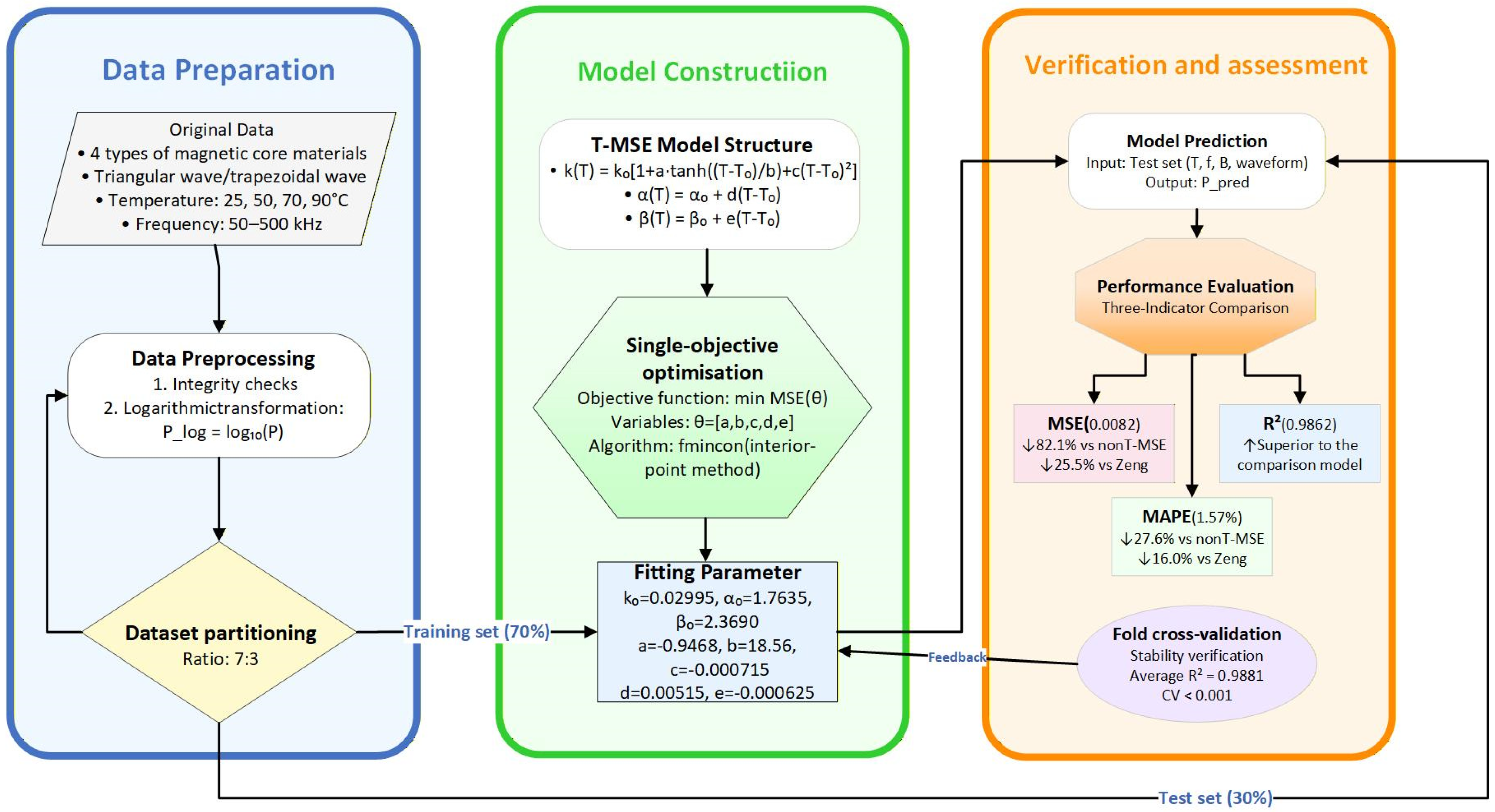
To clearly summarize the workflow proposed in this study, a comprehensive prediction framework is illustrated in Figure 1. This framework encompasses the entire process from raw data input to final model validation, which can be divided into three main stages: (1) Data preparation and preprocessing; (2) T-MSE model construction and parameter optimization; (3) Model performance evaluation and stability verification. The key step of partitioning the dataset into training and testing subsets with a 7:3 ratio, as described in Section 4.2, is explicitly highlighted. This schematic provides a clear roadmap for the following validation and discussion sections.

4. Verification

4.1. Data Sources

The core loss data for this study originates from Problem C in the 21st Huawei Cup China Postgraduate Mathematical Modelling Competition 2024, comprising loss experiment data for four core materials (Material 1, Material 2, Material 3, and Material 4). Although their specific compositions are not disclosed, these materials exhibit a range of loss characteristics (as shown in Table 1), providing a representative set to validate the model’s generalization capability. Sample characteristics for each material include temperature (T), frequency (f), excitation waveform, magnetic flux density (B), and core loss (P). For magnetic flux density, 1024 sampling points were recorded (equally spaced within one cycle duration), with the peak magnetic flux density (Bm) selected as the research feature. The excitation waveforms in the original dataset comprised both triangular and trapezoidal waves, which are typical non-sinusoidal waveforms. A thorough integrity check confirmed no missing values across all samples, indicating high data quality suitable for direct use in subsequent modeling and analysis.
The data for the four core materials are presented in Table 1. The “Sample Size” indicates the number of individual data points in the provided dataset, each representing a core loss value under a specific combination of conditions (temperature, frequency, waveform, and flux density). Sufficient sample quantities were obtained for each material, with frequencies exceeding 50 kHz, falling within the high-frequency excitation range. The measurements span multiple temperature levels from 25 °C to 90 °C, providing a comprehensive data foundation for investigating the influence of temperature on core loss.

4.2. Data Processing

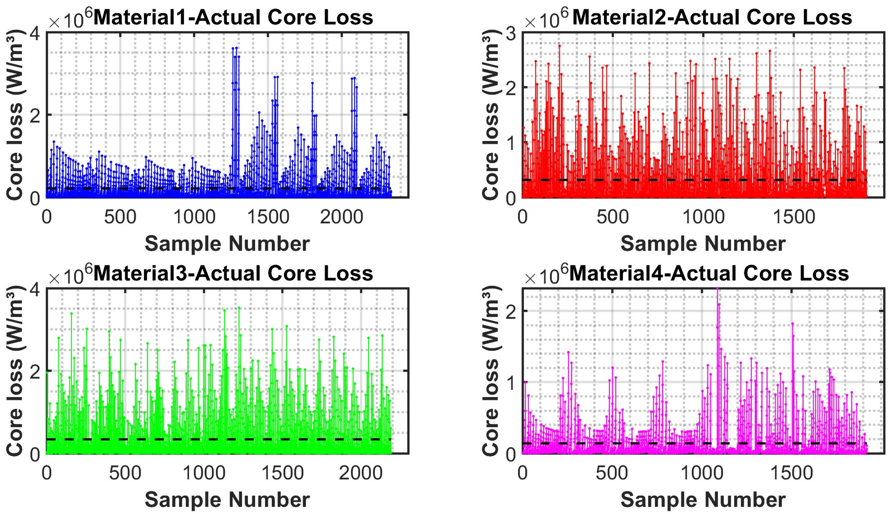
As outlined in Section 3, to ensure the validity of model training and evaluation, critical preprocessing was applied to the data before model fitting, alongside a rigorous dataset partitioning strategy. The four materials’ core losses are shown in Figure 2. Core loss exhibits an extremely wide dynamic distribution under high-frequency non-sinusoidal excitation conditions (e.g., the range of raw data for Material 1 reached 3.61 × 10⁶ W/m3). This high dynamic range gives rise to two major issues: firstly, when directly employed for model training, the errors from high-loss samples tend to “drown out” those from low-loss samples, causing parameter fitting to skew towards the high-loss range; secondly, numerical computations become prone to overflow or gradient anomalies, compromising the stability and convergence efficiency of optimization algorithms such as fmincon().
To reduce the range of data, the core loss data is subjected to a logarithmic transformation to base 10 [37]:
P log = l o g 10 max P , 10 20
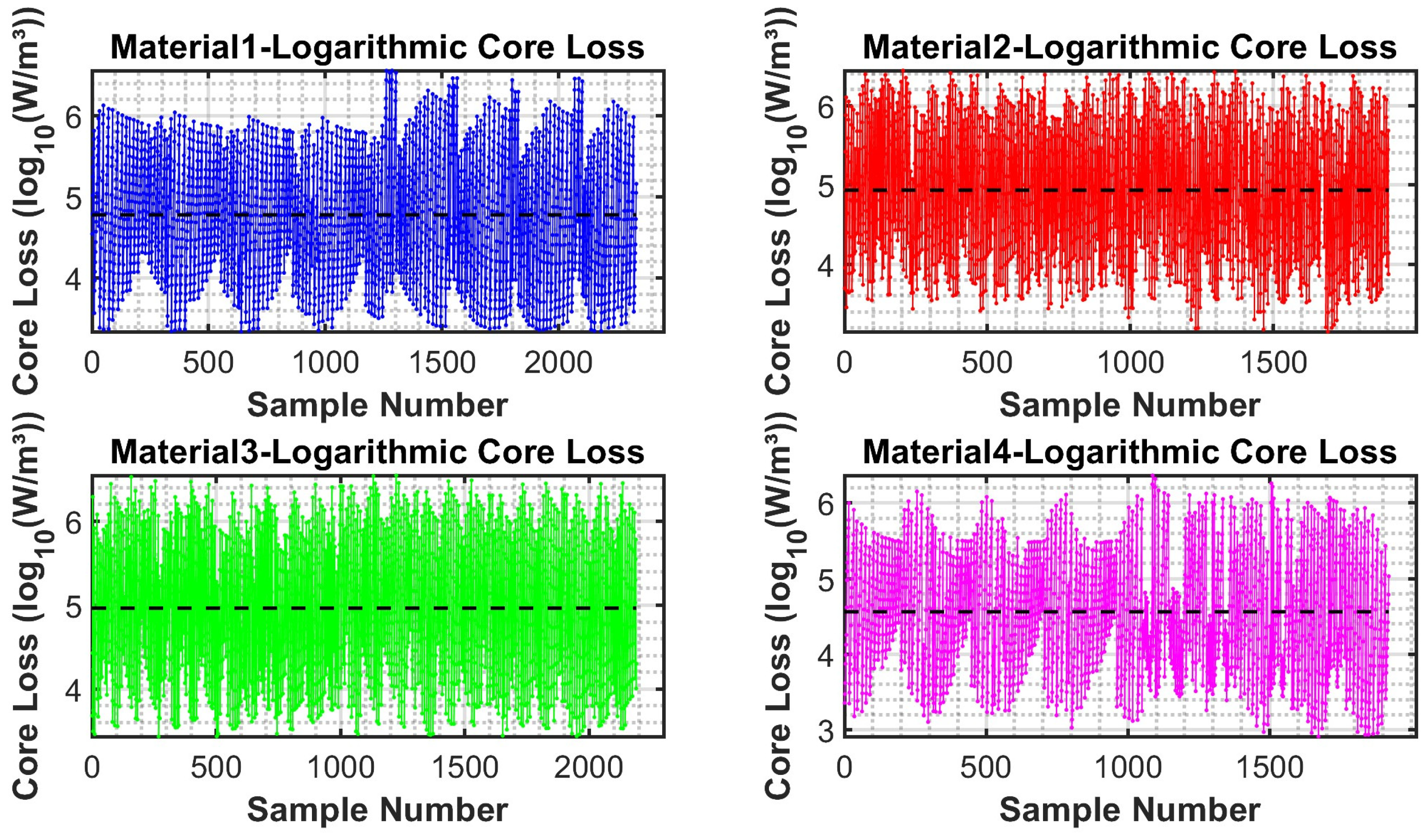
where P denotes the core loss (W/m3); max(P, 10−20) serves as a safety mechanism to handle cases where P approaches zero, preventing negative infinity values and ensuring the validity and stability of numerical operations. The processed data results are shown in Figure 3.
Comparing Figure 2 and Figure 3, the range of raw data for Material 1 is significantly compressed from 3.61 × 10⁶ W/m3 to 3.22 log10(W/m3) in the logarithmic domain. This adjustment balances the weighting of high- and low-loss samples in the model fitting process, preventing high-loss samples from unduly dominating the parameter identification procedure.
To ensure the impartiality and generalizability of model evaluation, following data preprocessing, a stratified random sampling strategy was employed to divide the datasets for the four core materials into training and test sets in a 7:3 ratio. The stratification employed temperature (25 °C, 50 °C, 70 °C, 90 °C) as the stratification variable, ensuring proportional sample distribution across each temperature stratum to mitigate evaluation bias arising from uneven temperature distribution. The training set is employed for model parameter identification and fitting, minimizing the deviation between predicted and actual loss through optimization algorithms to determine key parameters such as a, b, c, d, and e. The test set remained entirely independent, serving solely for the final evaluation of the model’s predictive performance and generalization capability. All performance metrics and comparative analyses reported herein are strictly based on calculations derived from the test set.

4.3. Evaluation Indicators

To comprehensively evaluate the predictive performance of the temperature correction model, taking into account the high dynamic range characteristics of the data, the following three metrics shall be employed:
  • Mean Square Error (MSE)
MSE serves as the core objective function for model parameter optimization, quantifying the overall error level of the model by calculating the MSE of the prediction [38]:
MSE = 1 n i = 1 n P pred , i P actual , i 2
The greater the MSE, the greater the discrepancy between the predicted and actual values, and the lower the accuracy.
2.
Mean Absolute Percentage Error (MAPE)
MAPE is the most intuitive relative error metric in engineering practice, expressed as a percentage reflecting the ratio of predicted error to actual loss [39]:
MAPE = 1 n i = 1 n P pred , i P actual , i P actual , i 100 %
The smaller the MAPE, the lower the relative error of the model and the higher its accuracy.
3.
Coefficient of Determination (R2)
R2 measures a model’s ability to explain trends in loss data, typically ranging from [0, 1]. Its core principle lies in quantifying the model’s fit to the data through the ratio of the sum of squared residuals to the total sum of squared deviations [40]:
R 2 = 1 i = 1 n P pred , i P actual , i 2 i = 1 n P pred , i P ¯ actual , i 2
where P ¯ a c t u a l , i denotes the mean of the true values. The closer R2 approaches 1, the more accurately the model captures the loss trend, the stronger its generalization capability, and the better its fitting performance.

4.4. Comparison of Logarithmic Processing in the T-MSE Model

Based on the aforementioned data partitioning and model training framework, the optimal model parameters are obtained through an optimization algorithm. The T-MSE model fitting parameters for each material after logarithmic transformation are presented in Table 2.
Table 2 demonstrates that the T-MSE model parameters for all four materials satisfy physical constraints: the a values range from −0.94 to −0.98 (ensuring k decreases with temperature), the d values range from 0.005 to 0.007 °C−1 (ensuring α increases with temperature), and the e values range from −0.00001 to −0.0006 °C−1 (ensuring β decreases with temperature), validating the physical plausibility of the parameter fitting. To verify the effectiveness of the logarithmic transformation, the core loss prediction results from the T-MSE model are compared between data with and without logarithmic transformation, as shown in Table 3.
Table 3 demonstrates that following logarithmic transformation, the predictive accuracy of the four materials improved by an order of magnitude—the MSE plummeted from “109” to the “10−2 order of magnitude”. For instance, Material 1’s MSE decreased from 4.08 × 10⁹ to 0.0073, representing an error reduction exceeding 5.6 × 10¹¹ times. MAPE generally contracted from the “15–17% range” to the “1.5–1.7% range”; Material 4’s MAPE decreased from 16.44% to 1.65%, representing a relative error reduction exceeding 90%; R2 exceeded 0.98 across all cases, ranging from a minimum of 0.9842 for Material 3 to a maximum of 0.9870 for Material 1, with an average R2 of 0.9858. This significantly enhanced the model’s explanatory power for core loss variations. The core reason for this performance leap lies in: The relationship between core loss and temperature, frequency, and magnetic flux density follows a power-law distribution. Logarithmic transformation converts multiplicative power-law relationships into additive linear relationships. This not only aligns with the mathematical structure of the T-MSE model but also compresses the dynamic range of the original data. This prevents high-loss samples from “weight suppression” over low-loss samples, ensuring balanced learning across the entire loss range. In summary, applying logarithmic transformation to magnetic core loss data—by converting multiplicative power-law relationships into additive linear relationships—constitutes a critical data processing strategy for enhancing the accuracy and robustness of the T-MSE model.

4.5. Multi-Material, Multi-Model Results Comparison

To comprehensively validate the T-MSE model (Equation (5)), it was compared against the nonT-MSE model (Equation (3)) [11] and the Zeng model (Equation (4)) [28]. The specific parameter values for the nonT-MSE model and the Zeng model are detailed in Table 4 and Table 5, respectively. Performance comparisons across the three models focused on MSE, MAPE, and R2.
For the four materials, the computational results of the nonT-MSE model, the T-MSE model, and the Zeng model are presented in Table 6. Firstly, the T-MSE model achieved optimal performance across all evaluation metrics for all four materials, demonstrating exceptional universality and stability. The average MSE across the four material groups was 0.0082, the average MAPE was 1.57%, and the average R2 reached 0.9862. In comparison, the Zeng model recorded an average MSE of 0.0110, average MAPE of 1.87%, and average R2 of 0.9807; while the nonT-MSE model achieved an average MSE of 0.0459, average MAPE of 2.17%, and average R2 of 0.9731. The T-MSE model’s mean MSE (0.0082) represents reductions of 25.5% and 82.1% relative to the Zeng model (0.0110) and the nonT-MSE model (0.0459), respectively. Its mean MAPE (1.57%) is similarly markedly lower than both counterparts (1.87%, 2.17%).
Secondly, the nonT-MSE model exhibited the most pronounced performance variation, with its MSE being exceptionally high on Material 1 (0.132), approximately seven to eight times that of other materials. This indicates that global parameter models are particularly vulnerable when confronted with materials exhibiting strong temperature sensitivity, such as Material 1. The Zeng model, employing a single temperature factor for global correction, stabilized performance to some extent (MSE range 0.0098–0.0119). However, its improvement proved limited, with MAPE rebounding above 2% on Material 4, indicating bottlenecks in its corrective capacity across varying material characteristics.
It is particularly noteworthy that the T-MSE model demonstrates optimal stability while maintaining the highest precision. The maximum and minimum values of its MSE differ by merely 0.0035, exhibiting far less fluctuation than the Zeng model (0.0021) and the nonT-MSE model (0.1245). Particularly concerning the coefficient of determination R2, the T-MSE model consistently stabilizes above 0.9842 across all materials (averaging 0.9862).
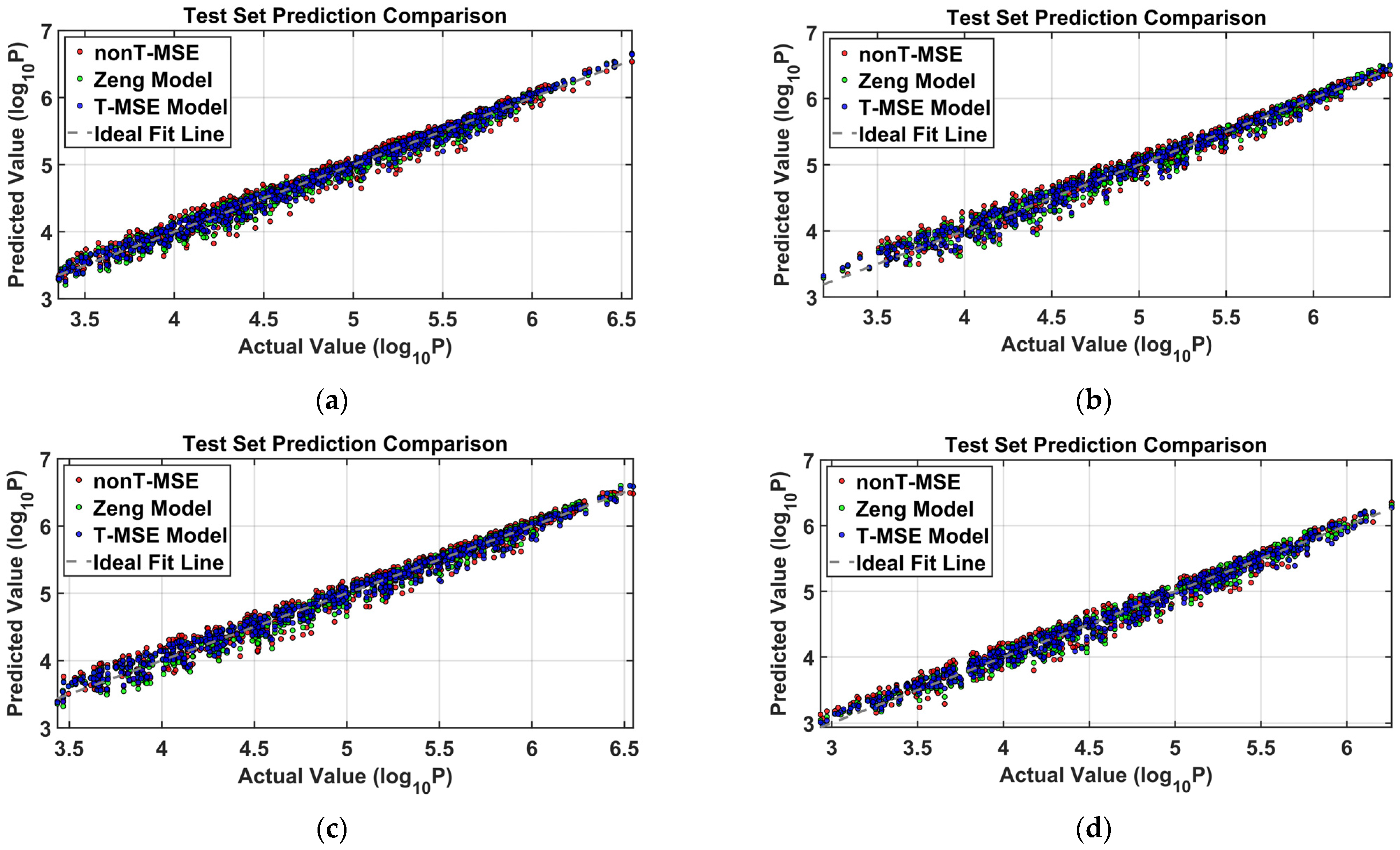
Figure 4 compares the predictive performance of different models. The T-MSE model’s predicted points (blue) cluster most closely around the ideal fit line (y = x), demonstrating excellent global consistency. In contrast, the nonT-MSE model exhibits a pronounced systematic “S”-shaped deviation, with significant overestimation particularly in the high-loss regions of Materials 2 and 4. Although the Zeng model’s predicted points are closer to the ideal line than the nonT-MSE model, a slight yet discernible negative deviation persists in the high-loss regions of Materials 1 and 4.
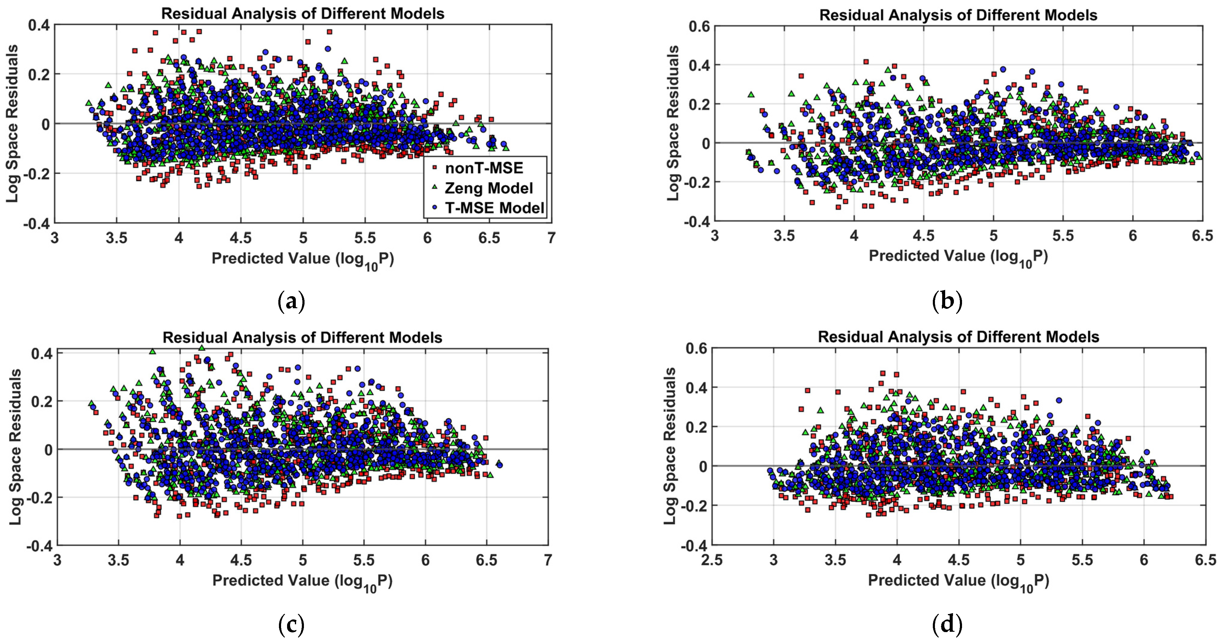
Simultaneously, in logarithmic space in Figure 5, the residuals of the T-MSE model exhibit the narrowest fluctuation range and are randomly distributed near the zero line, with no discernible systematic bias. This demonstrates its robust predictive capability across different loss magnitudes. By contrast, the Zeng model performed best on Material 3, with its residual distribution (Figure 5c) being more concentrated, narrowing the performance gap with the T-MSE model to 22.1%. However, for Material 4, the Zeng model’s performance declined, exhibiting increased residual fluctuation and widening the gap with T-MSE to 52.6%. Concurrently, the residual plots of the nonT-MSE model clearly reveal its systematic error: a consistent negative bias (underestimation) across low loss ranges, coupled with a pronounced positive bias (overestimation) in high loss ranges.
In summary, the T-MSE model not only surpasses the comparative models in prediction accuracy by modeling the temperature characteristics of the core parameters (k, α, β), but also demonstrates robustness and stability when applied to different magnetic materials. Its multi-parameter temperature correction framework effectively captures the distinct temperature dependencies of the Steinmetz parameters, thereby overcoming the limitations of both the fixed-parameter nonT-MSE model and the single-factor-corrected Zeng model. The model’s consistent and reliable performance is further corroborated by its minimal residual bias and excellent fit to the experimental data, offering a more reliable solution for accurate core loss prediction under high-frequency non-sinusoidal excitation.

4.6. Model Stability Validation

The aforementioned content evaluated the predictive performance of the T-MSE model based on a single training-test split. To ensure this superior performance dose not stem from the randomness of a particular data partition and to systematically assess the stability of model parameter estimation and generalization capability, five-fold cross-validation was subsequently conducted.
Cross-validation employed a stratified sampling strategy, using temperature (25 °C, 50 °C, 70 °C, 90 °C) as the stratification variable to ensure consistent temperature distribution within each fold relative to the full dataset. The specific procedure was as follows: (1) Randomly partition the dataset into five mutually exclusive subsets; (2) Successively designate each subset as the test set, with the remaining four serving as the training set, to independently perform parameter fitting and performance evaluation for the T-MSE model; (3) Repeat this process five times to ensure each subset undergoes one validation cycle; (4) Record the model performance metrics (R2, MSE, MAPE) and fitted parameters for each fold.
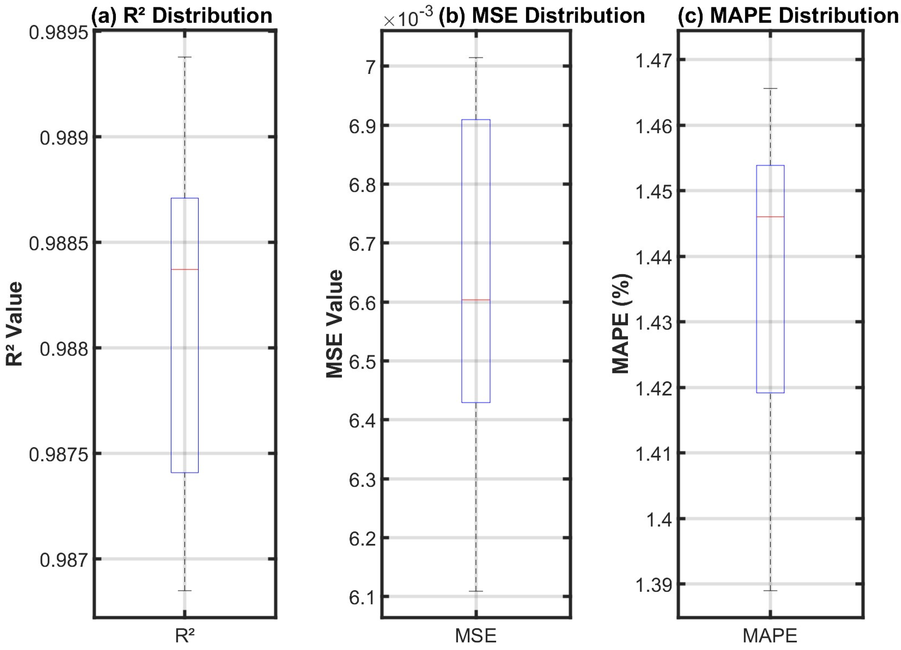
Taking the data from Material 1 as representative, the statistical results in Table 7 of the five-fold cross-validation performance metrics clearly demonstrate the T-MSE model’s exceptional stability across different data subsets. The core metric, the coefficient of determination R2, achieved an average value of 0.9881, with a standard deviation of merely 0.0010 and a coefficient of variation as low as 0.0010. Similarly, the coefficients of variation for MSE and MAPE are 0.0528 and 0.0134, respectively. These exceptionally low coefficients of variation demonstrate that the model’s predictive performance is insensitive to data partitioning, exhibiting robust generalization capabilities.
Figure 6 visually illustrates the distribution of the aforementioned performance metrics across the 50% threshold using box plots. It can be observed that the fluctuation range for all metrics is extremely narrow, with no outliers present, visually confirming the consistency of the model’s performance.
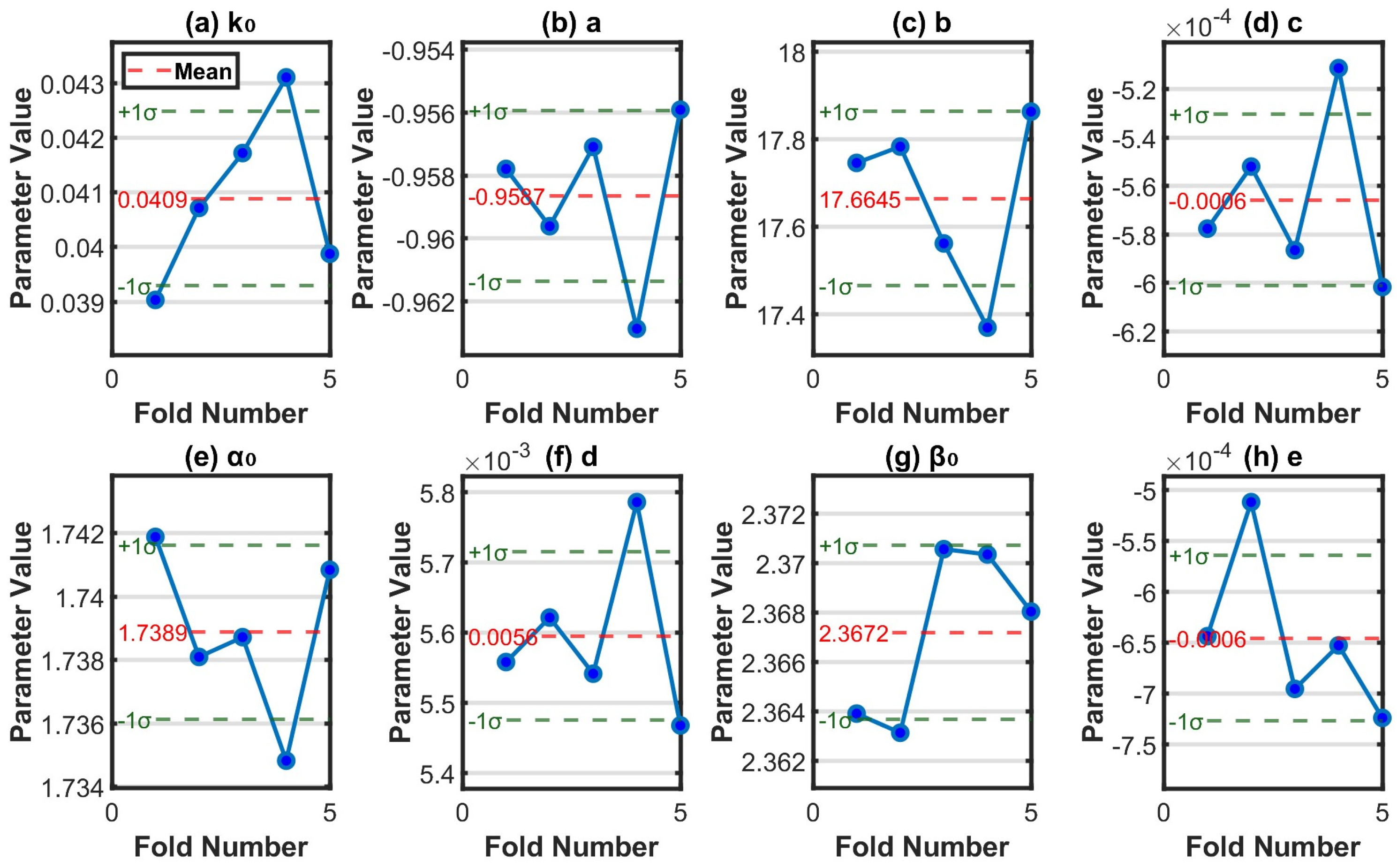
Table 8 presents the statistical results of the eight core parameters of the T-MSE model under five-fold cross-validation. The mean coefficient of variation for all parameters was 0.0329, demonstrating excellent overall stability. The coefficients of variation for the baseline frequency index α0 and baseline flux sensitivity coefficient β0 are low at 0.0016 and 0.0015, respectively, indicating high reproducibility of the model’s fundamental parameters. The coefficients of variation for the temperature correction parameters a and b are 0.0028 and 0.0111, respectively, likewise exhibiting stability.
Figure 7 visually illustrates the fluctuation patterns of each parameter across the five-fold cross-validation through a parameter variation trend chart. All data points cluster closely around their respective mean values, with fluctuations generally confined within ±1 standard deviation. Specifically, the baseline loss coefficient (k0), frequency exponent (α0), and flux density exponent (β0) demonstrate notably tight clustering around their central values. Among the temperature-correction terms, parameters a and b, which govern the nonlinear adjustment, show minimal dispersion. Parameters d (for α) and e (for β), representing linear temperature dependencies, display slightly broader but still confined variations. Parameter c exhibits the most visible fluctuation in the plot, consistent with its role in fine-tuning the saturation characteristic of the correction.
The five-fold cross-validation confirms that the T-MSE model is robust and not an artifact of a particular train-test split, thereby substantiating its reliability for practical application.

4.7. Discussion of Results

The experimental comparisons and stability analyses presented above provide several insights into the performance and characteristics of the T-MSE model, which are further discussed in this section.
The logarithmic transformation [40] applied to the core loss data played a crucial role in enhancing model accuracy. By compressing the wide dynamic range of loss values, this preprocessing step prevents high-loss samples from dominating the optimization objective. The transformation also aligns with the power-law structure of Steinmetz-based equations, effectively converting multiplicative relationships into additive forms in logarithmic space. As shown in Section 4.4, this approach significantly reduced prediction errors and improved the statistical reliability of parameter estimation.
The systematic comparison of the T-MSE, nonT-MSE, and Zeng models across four materials reveals distinct performance characteristics rooted in their structural formulations. The nonT-MSE model [11], while providing a foundation for handling non-sinusoidal waveforms, employs fixed, temperature-independent parameters. This fundamental limitation leads to systematic prediction errors, particularly under high-loss conditions and across varying temperatures, as reflected by its notable performance extremes: a maximum MSE of 0.132 (Material 1) and a maximum MAPE of 2.38% (Material 4), coupled with a minimum R2 of 0.9705 (Material 4). Residual analysis further reveals its consistent tendency to underestimate at low loss levels and overestimate at high loss levels.
The Zeng model [28] introduces a global square-root temperature correction factor, which improves prediction accuracy over the nonT-MSE model, achieving an average MSE of 0.0110 and MAPE of 1.87%. However, its single-parameter correction approach cannot fully capture the distinct temperature dependencies of the individual parameters (k, α, β). This structural distinction highlights why the multi-parameter T-MSE framework achieves more consistent accuracy across materials than the single-factor Zeng correction. Consequently, its performance varies across materials; while it demonstrates favorable adaptability for Material 3 (MSE = 0.0116, MAPE = 1.82%), a marked decline is observed for Material 4 (MSE = 0.0119, MAPE = 2.03%). This highlights the inherent limitations of a simplistic global correction when faced with diverse material microstructures.
In contrast, the T-MSE model employs a dedicated multi-parameter temperature correction framework, applying a nonlinear Tanh-based function to the loss coefficient k and linear corrections to the exponents α and β. This refined structure, while introducing more fitting parameters (eight in total) than the comparative models, enables a more accurate representation of the temperature-dependent loss behavior. The results presented in Section 4.5 confirm the effectiveness of this approach: despite the increased parameterization, the T-MSE model does not exhibit signs of overfitting in these experiments. Instead, it achieves remarkable performance extremes across all four tested materials: a minimum MSE of 0.0063 (Material 1), a minimum MAPE of 1.40% (Material 1), and a maximum R2 of 0.9888 (Material 1). This, coupled with its stable performance in cross-validation (Section 4.6), demonstrates its robust generalization capability. The additional computational cost associated with parameter identification thus represents a justified trade-off for the obtained gain in prediction accuracy. Furthermore, as illustrated by the residual analysis in Figure 4, its prediction residuals are randomly distributed with minimal systematic bias, demonstrating consistent performance across different loss levels and material types.
Furthermore, the five-fold cross-validation confirms the robustness of the T-MSE model. The model exhibits consistently low variability across different data partitions, as evidenced by key metrics: the coefficient of variation (CV) for R2 is merely 0.0010, and the mean CV for its eight core parameters is 0.0329. The average predictive performance across folds remained high, with a mean R2 of 0.9881 and a MAPE of 1.44% ± 0.03% in logarithmic space. These low variability measures indicate that the model’s performance is highly reproducible and insensitive to the specific split of the dataset. This stability, combined with high accuracy across diverse materials, supports the model’s reliability and generalizability for practical applications in power electronics design.
In summary, the T-MSE model demonstrates superior accuracy, robustness, and stability in predicting core loss under high-frequency non-sinusoidal excitation across a range of temperatures. Its performance advantage stems from a dedicated, multi-parameter temperature correction strategy and appropriate data preprocessing, making it a reliable analytical tool for the design and optimization of magnetic components in advanced power electronics.

5. Conclusions

Accurate prediction of core loss under high-frequency non-sinusoidal excitation is a critical engineering challenge, where temperature effects are significant. To address this, this study develops a novel T-MSE model. The core of this advancement is a dedicated multi-parameter temperature correction framework: it applies a nonlinear correction, combining a Tanh function with a quadratic decay term, to the loss coefficient k, while introducing linear correction terms for the frequency exponent α and flux density exponent β. This structure is designed to physically capture the distinct temperature dependencies inherent to different loss mechanisms.
The proposed model, supported by a logarithmic transformation of the wide-dynamic-range loss data and a single-objective optimization for parameter identification, demonstrates superior predictive performance. Comprehensive validation using experimental data from four distinct magnetic core materials confirms its accuracy and robustness. On the independent test set, the T-MSE model achieved average metrics of MSE = 0.0082, MAPE = 1.57%, and R2 = 0.9862. This represents a substantial improvement over both the nonT-MSE model (average MSE = 0.0459, MAPE = 2.17%, R2 = 0.9731) and the Zeng model (average MSE = 0.0110, MAPE = 1.87%, R2 = 0.9807), corresponding to a reduction in average prediction error of over 25%. The model’s excellent stability was further verified via five-fold cross-validation, yielding a mean R2 of 0.9881 with a coefficient of variation below 0.001.
Therefore, the primary contribution of this work is the development and rigorous validation of a practical, physics-informed T-MSE model. This model effectively and systematically integrates temperature effects into core loss prediction for high-frequency non-sinusoidal conditions, providing a more accurate and reliable analytical tool for the design and optimization of magnetic components in advanced power electronics.
The main limitation remains the model’s data-driven nature, requiring material-specific parameter fitting. Future work will aim to correlate the model’s coefficients with fundamental material properties and microstructural characteristics, paving the way for a more generalizable prediction framework. Additionally, comparison with well-established simulation models across different platforms could further strengthen the validation and practical utility of the proposed framework.

Author Contributions

Conceptualization, J.Z.; methodology, J.Z.; software, J.Z.; validation, Y.D. and C.L.; formal analysis, C.L.; investigation, J.Z.; resources, J.C.; data curation, J.Z. and C.L.; writing—original draft preparation, C.L. and J.Z.; writing—review and editing, C.L. and J.Z.; visualization, J.Z. and Y.D.; supervision, C.L.; project administration, C.L.; funding acquisition, J.C. All authors have read and agreed to the published version of the manuscript.

Funding

This work was supported by the Jiangsu Provincial Postgraduate Research and Practice Innovation Program Fund (SJCX24_2216).

Data Availability Statement

Restrictions apply to the availability of these data. Data were obtained from “The Huawei Cup” the 21st China Postgraduate Mathematical Modeling Competition, Problem C and are available Official Website of the China post-graduate mathematical contest in modeling Competition with the permission of Organizer.

Conflicts of Interest

The authors declare no conflicts of interest.

Nomenclature

The following symbols and abbreviations are used in this manuscript.
Symbols
SymbolDescriptionUnit
TTemperature°C
fExcitation frequencyHz
BMagnetic flux densityT
BmPeak magnetic flux densityT
ΔBPeak-to-peak magnetic flux densityT
PCore loss densityW/m3
kLoss coefficient in Steinmetz-based equations-
αFrequency exponent in Steinmetz-based equations-
βFlux density exponent in Steinmetz-based equations-
k0, α0, β0Reference values of k, α, β at T0 = 25 °C-
a, b, cFitting parameters for the nonlinear temperature correction of k(T)varied
d, eFitting parameters for the linear temperature correction of a(T) and β(T)varied
fsin.eqEquivalent frequency in nonT-MSE modelHz
ϕ(T)Temperature correction factor in Zeng model-
zFitting parameter in Zeng model’s correction factor-
Abbreviations
AbbreviationFull Name
SESteinmetz Equation
nonT-MSEModified Steinmetz Equation (without explicit temperature correction)
T-MSETemperature-corrected Modified Steinmetz Equation (proposed model)
Zeng modelThe square-root temperature-corrected MSE model proposed by Zeng et al.
GSEGeneralized Steinmetz Equation
iGSEImproved Generalized Steinmetz Equation
NSENatural Steinmetz Extension
MSEMean Square Error
MAPEMean Absolute Percentage Error
R2Coefficient of Determination

References

  1. Ravindran, R.; Massoud, A.M. An Overview of Wide and Ultra Wide Bandgap Semiconductors for Next-Generation Power Electronics Applications. Microelectron. Eng. 2025, 300, 112374. [Google Scholar] [CrossRef]
  2. Chaudhary, O.S.; Denai, M.; Refaat, S.S.; Pissanidis, G. Technology and Applications of Wide Bandgap Semiconductor Materials: Current State and Future Trends. Energies 2023, 16, 6689. [Google Scholar] [CrossRef]
  3. Imaoka, J.; Wu, Y.H.; Shigematsu, K.; Aoki, T.; Noah, M.; Yamamoto, M. Effects of High-frequency Operation on Magnetic Components in Power Converters. In Proceedings of the 2021 IEEE Energy Conversion Congress and Exposition—Asia (ECCE-Asia), Singapore, 24–27 May 2021; pp. 978–984. [Google Scholar]
  4. Dawood, K.; Kul, S. Influence of Core Window Height on Thermal Characteristics of Dry-Type Transformers. Case Stud. Therm. Eng. 2025, 66, 105746. [Google Scholar] [CrossRef]
  5. Boehning, L.; Schwalbe, U. Modelling and loss simulation of magnetic components in power electronic circuit by impedance measurement. In Proceedings of the International Exhibition and Conference for Power Electronics, Intelligent Motion, Renewable Energy and Energy Management: International Exhibition and Conference for Power Electronics, Intelligent Motion, Renewable Energy and Energy Management, Nuremburg, Germany, 7–8 July 2020; pp. 1–7. [Google Scholar]
  6. Chen, J.; Du, X.; Luo, Q.M.; Zhang, X.Y.; Sun, P.J.; Zhou, L. A Review of Switching Oscillations of Wide Bandgap Semiconductor Devices. IEEE Trans. Power Electron. 2020, 35, 13182–13199. [Google Scholar] [CrossRef]
  7. Ma, C.-T.; Gu, Z.-H. Review on Driving Circuits for Wide-Bandgap Semiconductor Switching Devices for Mid- to High-Power Applications. Micromachines 2021, 12, 65. [Google Scholar] [CrossRef]
  8. Hanson, A. Opportunities in magnetic materials for high-frequency power conversion. MRS Commun. 2022, 12, 521–530. [Google Scholar] [CrossRef]
  9. Leaky, A.M.; Ohodnicki, P.R.; McHenry, M.E. Soft Magnetic Materials in High-Frequency, High-Power Conversion Applications. JOM 2012, 64, 772–781. [Google Scholar]
  10. Steinmetz, C.P. On the law of hysteresis. Proc. IEEE 1984, 72, 197–221. [Google Scholar] [CrossRef]
  11. Reinert, J.; Brockmeyer, A.; De Doncker, R.W.A.A. Calculation of losses in ferro-and ferrimagnetic materials based on the modified steinmetz equation. IEEE Trans. Ind. Appl. 2001, 37, 1055–1061. [Google Scholar] [CrossRef]
  12. Li, J.; Abdallah, T.; Sullivan, C.R. Improved calculation of core loss with nonsinusoidal waveforms. In Proceedings of the Conference Record of the 2001 IEEE Industry Applications Conference. 36th IAS Annual Meeting (Cat. No.01CH37248), Chicago, IL, USA, 30 September–4 October 2001. [Google Scholar]
  13. Venkatachalam, K.; Sulivan, C.R.; Abdallah, T.; Tacca, H. Accurate prediction of ferrite core loss with nonsinusoidal waveforms using only Steinmetz parameters. In Proceedings of the 2002 IEEE Workshop on Computers in Power Electronics (COMPEL 2002), Mayaguez, PR, USA, 3–4 June 2002; pp. 36–41. [Google Scholar]
  14. Detka, K.; Górecki, K. Modelling power losses in an inductor contained in the boost converter. In Proceedings of the 2018 12th International Conference on Compatibility, Power Electronics and Power Engineering (CPE-POWERENG), Doha, Qatar, 10–12 April 2018; pp. 1–6. [Google Scholar]
  15. Bertotti, G. General properties of power losses in soft ferromagnetic materials. IEEE Trans. Magn. 1988, 24, 621–630. [Google Scholar] [CrossRef]
  16. Fiorillo, F.; Novikov, A. An improved approach to power losses in magnetic laminations under nonsinusoidal induction waveform. IEEE Trans. Magn. 1990, 26, 2904–2910. [Google Scholar] [CrossRef]
  17. Fiorillo, F.; Novikov, A. Power losses under sinusoidal, trapezoidal and distorted induction waveform. IEEE Trans. Magn. 1990, 26, 2559–2561. [Google Scholar] [CrossRef]
  18. Rodriguez-Sotelo, D.; Rodriguez-Licea, M.A.; Araujo-Vargas, I.; Prado-Olivarez, J.; Barranco-Gutiérrez, A.-I.; Perez-Pinal, F.J. Power Losses Models for Magnetic Cores: A Review. Micromachines 2022, 13, 418. [Google Scholar] [CrossRef]
  19. Górecki, K.; Detka, K. Improved Method for Measuring Power Losses in the Inductor Core. IEEE Trans. Instrum. Meas. 2021, 70, 1500710. [Google Scholar] [CrossRef]
  20. Alsawalhi, J.Y.; Sudhoff, S.D. Saturable Thermally-Representative Steinmetz-Based Loss Models. IEEE Trans. Magn. 2013, 49, 5438–5445. [Google Scholar] [CrossRef]
  21. Ono, N.; Uehara, Y.; Onuma, T.; Taniguchi, T.; Kikuchi, N.; Okamoto, S. Multimodal Iron Loss Analyses Based on Magnetization Processes for Various Soft Magnetic Toroidal Cores. J. Magn. Magn. Mater. 2024, 603, 172222. [Google Scholar] [CrossRef]
  22. Baek, S.; Lee, J.S. A multi-dimensional finite element analysis of magnetic core loss in arbitrary magnetization waveforms with switching converter applications. Electr. Eng. 2024, 106, 1793–1804. [Google Scholar] [CrossRef]
  23. Tumanski, S. A Method of Testing of the Plane Distribution of Anisotropy. IEEE Trans. Magn. 2002, 38, 2808–2810. [Google Scholar] [CrossRef]
  24. Kwiatkowski, W.; Stabrowski, M.; Tumanski, S. Numerical Analysis of the Shape Anisotropy and Anisotropy Dispersion in Thin Film Permalloy Magnetoresistors. IEEE Trans. Magn. 1983, 19, 2502–2505. [Google Scholar] [CrossRef]
  25. Tumanski, S.; Stabrowski, M.E. Numerical Calculations of Magnetization and Demagnetizing Factors in Thin Film Anisotropic Structures. IEEE Trans. Magn. 1988, 24, 222–225. [Google Scholar] [CrossRef]
  26. Tumanski, S.; Liszka, A. On-Line Evaluation of Electrical Steel Structure and Quality. In Proceedings of the 2002 IEEE International Magnetics Conference (INTERMAG), Amsterdam, The Netherlands, 28 April–2 May 2002; pp. 1212–1213. [Google Scholar] [CrossRef]
  27. Deng, M.W.; Yang, Y.Z.; Fu, P.X.; Liang, S.X.; Fu, X.L.; Cai, W.T.; Tao, P.J. Core-Loss Behavior of Fe-Based Nanocrystalline at High Frequency and High Temperature. J. Mater. Sci. Mater. Electron. 2024, 35, 856. [Google Scholar] [CrossRef]
  28. Zeng, Y.; Gong, D.; Zu, Y.T.; Zhang, Q. Temperature-Compensated Multi-Objective Framework for Core Loss Prediction and Optimization: Integrating Data-Driven Modeling and Evolutionary Strategies. Mathematics 2025, 13, 2758. [Google Scholar] [CrossRef]
  29. Sapkota, D.B.; Neupane, P.; Joshi, M.; Khan, S. Deep Learning Model for Enhanced Power Loss Prediction in the Frequency Domain for Magnetic Materials. IET Power Electron. 2024, 1–12. [Google Scholar] [CrossRef]
  30. Li, Z.; Wang, L.; Liu, R.; Mirzadarani, R.; Luo, T.; Lyu, D.; Ghaffarian Niasar, M.; Qin, Z. A Data-Driven Model for Power Loss Estimation of Magnetic Materials Based on Multi-Objective Optimization and Transfer Learning. IEEE Open J. Power Electron. 2024, 5, 605–617. [Google Scholar] [CrossRef]
  31. Rasekh, N.; Wang, J.; Yuan, X. Artificial Neural Network Aided Loss Maps for Inductors and Transformers. IEEE Open J. Power Electron. 2022, 3, 886–898. [Google Scholar] [CrossRef]
  32. Chen, G.; Li, Z.J.; Zhang, L.M.; Chang, Q.; Chen, X.J.; Fan, X.M.; Chen, Q.; Wu, H.J. Mechanisms, Design, and Fabrication Strategies for Emerging Electromagnetic Wave-Absorbing Materials. Cell Rep. Phys. Sci. 2024, 5, 102097. [Google Scholar] [CrossRef]
  33. Choi, M.W.; Park, S.Y.; Jang, E.Y.; Ouk, M.; Park, K.H.; Lee, S.W.; Noh, G. Fabrication-Specific Simulation of Mn-Zn Ferrite Core-Loss for Machine Learning-Based Surrogate Modeling With Limited Experimental Data. IEEE Trans. Power Electron. 2025, 40, 1519–1531. [Google Scholar] [CrossRef]
  34. Durna, E. Recursive inductor core loss estimation method for arbitrary flux density waveforms. J. Power Electron. A Publ. Korean Inst. Power Electron. 2021, 21, 1724–1734. [Google Scholar] [CrossRef]
  35. Mohammad, S.; Mendoza, I. A New Hyperbolic Tangent Family of Distributions: Properties and Applications. Ann. Data Sci. 2025, 12, 457–480. [Google Scholar] [CrossRef]
  36. Benhamida, F. A Solution Method to Economic Dispatch Using the Matlab Function (FMINCON). Model. Meas. Control. A Gen. Phys. Electron. Electr. Eng. 2006, 79, 1–13. [Google Scholar]
  37. Lu, C.; Meng, F.; Zhang, J.; Zhang, Z. Core Loss Prediction Model of High-Frequency Sinusoidal Excitation Based on Artificial Neural Network. Magnetochemistry 2025, 11, 93. [Google Scholar] [CrossRef]
  38. Koksoy, O. Multiresponse Robust Design: Mean Square Error (MSE) Criterion. Appl. Math. Comput. 2006, 175, 1716–1729. [Google Scholar] [CrossRef]
  39. De Myttenaere, A.; Golden, B.; Le Grand, B.; Rossi, F. Mean Absolute Percentage Error for Regression Models. Neurocomputing 2016, 192, 38–48. [Google Scholar] [CrossRef]
  40. Cheng, C.-L.; Shalabh; Garg, G. Coefficient of Determination for Multiple Measurement Error Models. J. Multivar. Anal. 2014, 126, 137–152. [Google Scholar] [CrossRef]
Figure 1. T-MSE Model Construction and Validation Workflow. The upward arrow indicates higher, the downward arrow indicates lower.
Magnetochemistry 12 00006 g001
Figure 2. Distribution of the raw core loss data for the four materials.
Magnetochemistry 12 00006 g002
Figure 3. Distribution of the core loss data after logarithmic transformation.
Magnetochemistry 12 00006 g003
Figure 4. Comparison of model predictive performance for different materials ((ad) represent Materials 1–4, respectively).
Magnetochemistry 12 00006 g004
Figure 5. Residual analysis of each model in logarithmic space for different materials ((ad) represent Materials 1–4, respectively).
Magnetochemistry 12 00006 g005
Figure 6. Distribution of performance metrics for five -fold cross-validation of the T-MSE model. (The blue boxplot represents the distribution of the corresponding performance metrics (R2, MSE, MAPE) in the five-fold cross-validation of the T-MSE model; the red line denotes the mean value of the metric in the five-fold validation; and the dashed line is used to assist in showing the fluctuation range of the metric.).
Magnetochemistry 12 00006 g006
Figure 7. Stability of T-MSE model parameters in five-fold cross-validation.
Magnetochemistry 12 00006 g007
Table 1. Statistical characteristics of experimental data for four core materials.
MaterialSample SizeTemperature (°C)Frequency (kHz)Peak Magnetic Flux Density (T)Core Loss (W/m3)
TotalTriangular WaveTrapezoidal Wave
Material 12333141292125, 50, 70, 90[50.06, 446.41][0.011, 0.279][2.186 × 10³, 3.616 × 10⁶]
Material 21903100390025, 50, 70, 90[49.99, 499.99][0.010, 0.313][1.413 × 10³, 2.750 × 10⁶]
Material 321901078111225, 50, 70, 90[49.99, 499.99][0.010, 0.313][2.723 × 10³, 3.525 × 10⁶]
Material 41920145546525, 50, 70, 90[50.06, 446.43][0.011, 0.278][8.158 × 10², 2.322 × 10⁶]
Table 2. Log-transformed T-MSE model fitting parameters for each material.
ParameterMaterial 1 Material 2Material 3Material 4
k00.0299520.2129190.4500490.124342
a−0.946845−0.967543−0.952768−0.977214
b18.55964917.48430218.37055615.874876
c−0.000715−0.000438−0.000626−0.000324
α01.7634931.6260441.5797511.710235
d0.0051530.0059960.0054520.006863
β02.3689792.3954172.4263542.493406
e−0.000625−0.000073−0.000011−0.000517
Table 3. Comparison of results from two data processing methods for the T-MSE model.
MaterialEvaluation IndicatorsWithout Logarithmic TransformationAfter Logarithmic Transformation
Material 1MSE4.08 × 1090.0073
MAPE15.32%1.50%
R20.97120.9870
Material 2MSE5.46 × 1090.0093
MAPE16.59%1.60%
R20.97430.9850
Material 3MSE9.18 × 1090.0095
MAPE16.98%1.61%
R20.96960.9842
Material 4MSE3.35 × 1090.0078
MAPE16.44%1.65%
R20.94120.9869
Table 4. Log-transformed nonT-MSE model fitting parameters for each material.
ParameterMaterial 1Material 2Material 3Material 4
k10.0025400.0143880.0402940.006219
α11.9339971.8220611.7540601.929358
β12.3313922.3823782.4138702.467184
Table 5. Log-transformed Zeng model fitting parameters for each material.
ParameterMaterial 1Material 2Material 3Material 4
k20.0032490.0177880.0488940.006857
α21.9375971.8262761.7586901.9449932
β22.310082.3818882.4145762.479762
z−0.044860−0.044418−0.042478−0.043130
Table 6. Results for each model under different materials.
MaterialEvaluation IndicatorsnonT-MSE ModelT-MSE ModelZeng Model
Material 1MSE0.1320.00630.0098
MAPE1.98%1.40%1.74%
R20.97650.98880.9824
Material 2MSE0.01770.00930.0125
MAPE2.23%1.60%1.87%
R20.97130.98500.9798
Material 3MSE0.01550.00950.0116
MAPE2.09%1.61%1.82%
R20.97420.98420.9807
Material 4MSE0.01750.00780.0119
MAPE2.38%1.65%2.03%
R20.97050.98690.9800
Table 7. Statistics on five-fold cross-validation performance metrics (Material 1).
IndicatorMeanStandard DeviationCoefficient of VariationMinimum ValueMaximum Value
R20.98810.00100.00100.98680.9894
MSE0.00660.00030.05280.00610.0070
MAPE (%)1.440.030.02041.391.47
Table 8. Stability analysis of T-MSE model parameters (Material 1).
ParameterMeanStandard DeviationCoefficient of VariationMinimum ValueMaximum Value
k00.0408890.0015890.0388540.0390330.043103
a−0.9589170.0027210.002838−0.963013−0.956158
b17.6488200.1966000.01114017.35958017.862757
c−0.0005620.0000350.063114−0.000598−0.000509
α01.7388790.0027360.0015741.7348311.741888
d0.0056060.0001210.0215190.0054750.005792
β02.3671940.0035100.0014832.3631292.370557
e−0.0006430.0000790.122913−0.000715−0.000513
Disclaimer/Publisher’s Note: The statements, opinions and data contained in all publications are solely those of the individual author(s) and contributor(s) and not of MDPI and/or the editor(s). MDPI and/or the editor(s) disclaim responsibility for any injury to people or property resulting from any ideas, methods, instructions or products referred to in the content.