Article

Multidimensional Evaluation of Sustainable Lettuce (Lactuca sativa L.) Production: Agronomic, Sensory, and Economic Criteria Using the Fuzzy PIPRECIA–Fuzzy MARCOS Model

by
Radomir Bodiroga
1,*,
Milena Marjanović
2,
Vuk Maksimović
3,
Đorđe Moravčević
2,
Zorica Jovanović
2,
Slađana Savić
4 and
Milica Stojanović
3,*
1
Faculty of Agriculture, University of East Sarajevo, 71123 East Sarajevo, Bosnia and Herzegovina
2
Faculty of Agriculture, University of Belgrade, 11080 Belgrade, Serbia
3
Institute for Multidisciplinary Research, National Institute of the Republic of Serbia, University of Belgrade, 11030 Belgrade, Serbia
4
Institute for Plant Protection and Environment, 11040 Belgrade, Serbia
*
Authors to whom correspondence should be addressed.
Horticulturae 2026, 12(3), 368; https://doi.org/10.3390/horticulturae12030368
Submission received: 6 February 2026 / Revised: 9 March 2026 / Accepted: 10 March 2026 / Published: 16 March 2026

Abstract

Although greenhouse vegetable production is rapidly shifting toward innovative soilless systems, soil-based conventional cultivation still dominates globally. This production system faces growing pressure to transition to sustainable practices. However, introducing biofertilisers into intensive systems often yields inconsistent results. Specifically, their effects on different lettuce traits vary due to complex relationships between genotype, biofertiliser, environmental conditions, and market demands. Single-parameter evaluations fail to balance conflicting criteria, necessitating multi-criteria decision-making (MCDM) methods for selecting optimal choices. This study aims to overcome these inconsistencies through an integrated fuzzy MCDM-based optimisation model. Three lettuce cultivars (‘Carmesi’, ‘Aquino’, and ‘Gaugin’) were grown in an unheated Surčin (Serbia) greenhouse during a 58-day autumn experiment using a complete block design. Four treatments were applied: a control (without fertilisation), effective microorganisms, a Trichoderma-based fertiliser, and their combination. Biofertilisers were applied before transplanting and four times foliarly during the vegetation period via battery sprayer. This defined 12 production models (cultivar–fertiliser pairs), evaluated across 10 criteria: agronomic (core ratio, number of leaves), quality (nitrate content, total antioxidant capacity, total soluble solids, and chlorogenic acid), sensory (overall taste, overall quality), and economic (total variable costs, total income). Four decision-making experts from the Faculty of Agriculture and the ready-to-eat salad industry assessed weighting coefficients using the fuzzy PIPRECIA (PIvot Pairwise RElative Criteria Importance Assessment) method. The fuzzy MARCOS (Measurement Alternatives and Ranking according to COmpromise Solution) method was used to rank the alternatives. To confirm the stability of the obtained ranking with the fuzzy MARCOS method, we performed sensitivity analysis through 20 different scenarios. Applied fuzzy methods identified alternative A11—‘Aquino’ cultivar with combined biofertilisers—as the best-ranked option, followed by A6 and A7. This study validates fuzzy PIPRECIA and fuzzy MARCOS as effective tools for optimising lettuce production models. They support farmers in selecting the most favourable solution based on multiple criteria, aiding the shift from mineral fertilisers to sustainable biofertiliser-based systems in intensive production—especially helpful for producers making this transition.

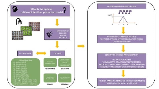
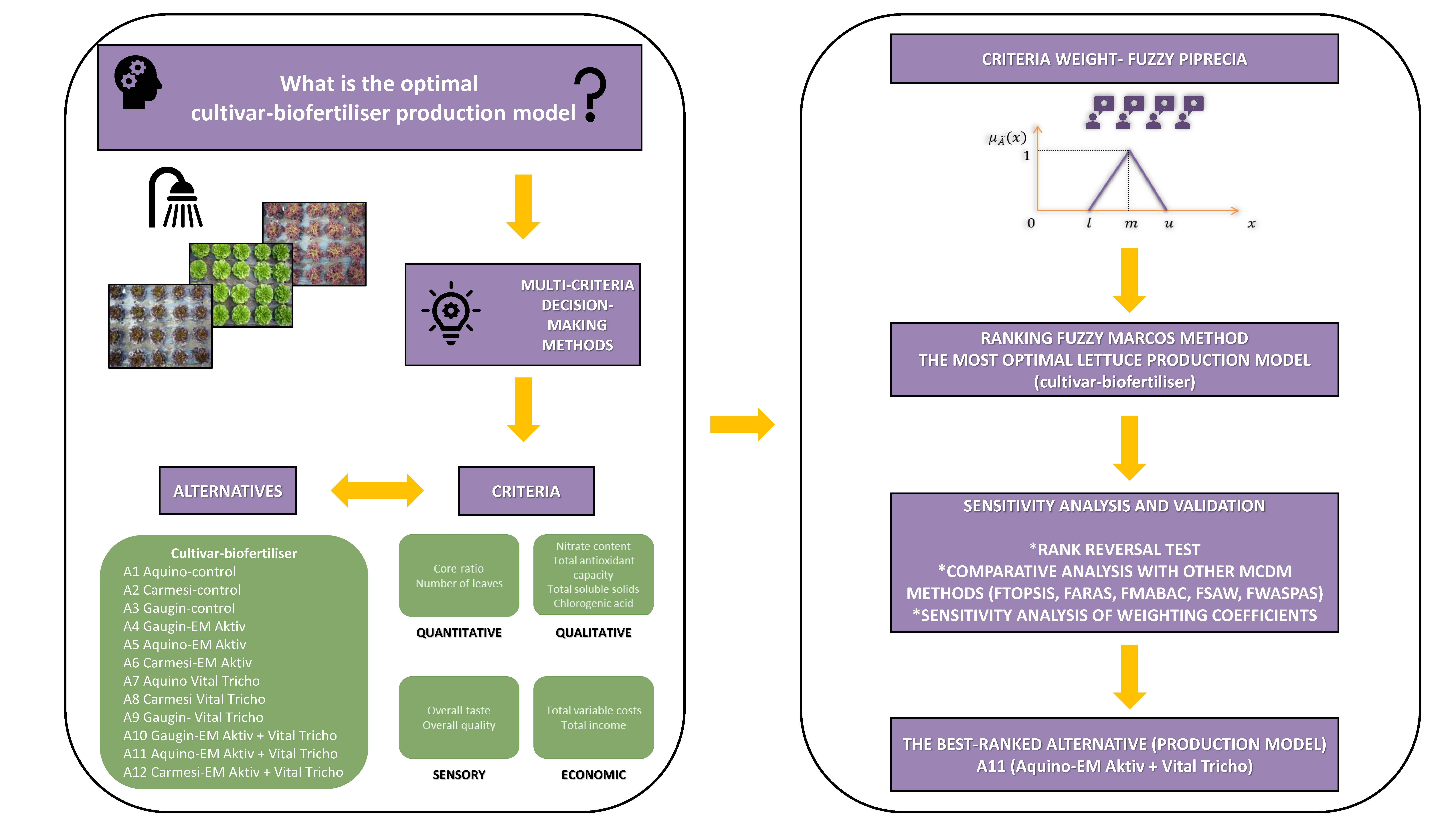
Graphical Abstract

1. Introduction

The fresh-cut fruit and vegetable industry has expanded significantly over the past decade across Europe. Per capita consumption of salad crops has grown in several European countries (Germany, France, Italy, the United Kingdom, and Spain) over the past decade, ranging from 0.7 to 1.7 kg per year in 2020, reflecting their popularity and strong consumer demand in this booming sector [1]. This increase is driven by shifts in modern lifestyles and growing demand for convenient, quick, and healthy meal options. Lettuce, one of the most popular leafy greens, offers substantial nutritional value and has a significant economic impact [2], due to high economic turnover and multiple harvests per year [3]. Its wide-ranging health benefits are derived from bioactive compounds, including flavonoids, phenolic acids, carotenoids, various vitamins, and sesquiterpene lactones, which contribute to antioxidant, anti-inflammatory, antidiabetic, anticancer, and antiviral effects [4].
According to FAO data [5] from 2020 to 2024, the European Union’s harvested lettuce and chicory area declined from 131.050 to 120.070 ha, while production quantities decreased from 3.645.170 to 3.257.930 tonnes. Official data on lettuce production in Serbia remain unavailable, despite its ranking among the country’s most extensively cultivated vegetable crops [6]. In neighbouring countries, data from the same period indicate decreasing harvested areas in most of them—except Croatia, Hungary, and Romania—while production quantities declined more broadly, affecting more countries, except in Hungary [5].
Lettuce is a cool-season crop that exhibits optimal growth at temperatures ranging from 15 to 25 °C [7]. In continental climate regions, it can be cultivated year-round through autumn, winter, and spring without using additional heating and lighting devices. Greenhouse systems permit higher productivity of crops per cultivation area compared to open-field systems through the possibility of production intensification [8,9]. As soil and water resources diminish amid rising global populations, greenhouse production proves indispensable for achieving maximum yields per unit area, independent of environmental limitations [10]. In Serbia, the most common greenhouse type is the affordable, unheated ‘Mediterranean’ style designed for soil-based crops, much like those widely used in Turkey [11].
Global agricultural productivity faces threats from plant diseases, inefficient chemical fertilisers, soil degradation, and water scarcity [12]. Excessive nitrogen application—essential for obtaining high yields—causes eutrophication, emissions, nitrate accumulation linked to the formation of nitrosamines and methemoglobinemia, and yield declines, while prolonged use of chemical fertilisers degrades soil health, disrupts soil microbes, and depletes soil fertility [13,14,15,16]. Sustainable solutions like biofertilisers offer a promising approach to enhance crop productivity and plant resilience, meeting rising lettuce demand during intensifying climate pressures [17,18].
Biofertilisers are products containing beneficial microorganisms isolated from plant roots and the rhizosphere, in active or dormant forms. They competitively colonise plant roots, enhancing nutrient uptake, crop yields, and productivity while boosting stress tolerance, pathogen resistance, and growth through nutrient mobilisation and plant hormones. Eco-friendly and cost-effective, they build soil biological activity over time and increase yields by 10–40% via nitrogen fixation and elevated levels of amino acids, proteins, and vitamins [19]. Trichoderma species, widely used as biocontrol agents against phytopathogenic microorganisms, promote plant growth and provide disease protection—often as endophytic fungi—via mechanisms such as enhanced nutrient access (e.g., nitrogen, phosphorus, potassium, zinc, iron), antibiotic and plant hormone production, ethylene reduction, and increased water acquisition [20]. These species further reduce reliance on mineral fertilisers by boosting soil microbial activity and nutrient availability [21]. Studies show that various Trichoderma species and other biofertilisers have positive effects on lettuce agronomic performance, including quantity and quality traits [22,23,24,25,26]. These biofertiliser effects guided our selection of 10 specific criteria for evaluating cultivar–biofertiliser performance.
These criteria directly reflect diverse stakeholder priorities across the lettuce value chain. Appearance, colour, and texture are the major marketable traits of fresh lettuce [27]. Both consumers and the processing industry prefer cultivars with more leaves, with consumer attention focused on appearance, volume, and secondarily, the number of leaves [28]. According to Maboko and Du Plooy [29], the core ratio (stem-to-rosette length) must not exceed 0.5—a key processing industry indicator of rosette use efficiency, which signals premature bolting and unfavourable growing conditions.
Consumers value quality traits, where lettuce’s health benefits partly derive from phenolics (phenolic acids and flavonoids). Chlorogenic acid—a common secondary metabolite in lettuce [30,31,32]—exhibits potent pharmacological activities, including different antioxidant and protective roles in both in vitro and in vivo studies [33]. Total soluble solids also play a key role in quality, as they influence taste [34]. While some bitterness is inherent to lettuce, consumers prefer less bitter, sweeter cultivars, increasing acceptance [35]. Identifying preferred organoleptic qualities could guide growers and breeders in cultivar selection [36].
Conventional agronomic statistical analyses determine significant differences between main factors (e.g., effects of cultivar or treatment). However, their application is limited when multiple parameters (criteria) must be considered simultaneously in decision-making to find optimal solutions. For instance, high-yielding cultivars may compromise processing quality standards. This makes single-parameter decision-making insufficient. Additional complexity arises from mixed quantitative and qualitative indicators, which carry inherent uncertainty. These scenarios significantly complicate choices, and in such situations, multi-criteria decision-making (MCDM) methods can provide significant help by making the decision-making process more explicit, rational, and efficient [37]. This methodological gap necessitates MCDM methods to integrate all criteria and rank cultivar–biofertiliser combinations comprehensively.
MCDM methods gained substantial attention across different sectors from 2012 to 2022, evidenced by 3.442 engineering publications compared to just 471 in agricultural and biological sciences [38]. According to Cicciù et al. [39], scientific papers on multi-criteria methods exploring agricultural sustainability grew markedly from 2016 to 2021, averaging six papers per year. MCDM methods are powerful analytical tools because they evaluate alternatives across conflicting criteria to identify optimal solutions. Traditional MCDM approaches, such as the Analytic Hierarchy Process (AHP), Technique for Order of Preference by Similarity to Ideal Solution (TOPSIS), and Elimination and Choice Translating Reality (ELECTRE), have demonstrated substantial effectiveness in complex decision problems [40]. These have evolved into advanced fuzzy logic, hybrid, and AI-driven systems [40]. MCDM methods incorporate both numerical and linguistic values, with the latter aligning closely with human cognition for intuitive expert assessments [41]. In agricultural decision-making, traditional binary logic (true/false, yes/no) fails to capture real-field data’s nuance and uncertainty, while fuzzy logic addresses this by representing gradations such as ‘high’, ‘medium’, or ‘low’, making it ideal for agriculture’s dynamic and imprecise conditions [42]. This methodology processes these linguistic inputs to address vagueness, mirroring human thinking when precise values are elusive [43].
Traditional crop production methods fail to handle agriculture’s dynamic variables—climate fluctuations, soil degradation, market demands, and resource constraints—causing inefficiencies that advanced decision-making tools must overcome to optimise productivity and sustainability. Fuzzy logic enables decisions across a range of possibilities rather than rigid binary choices, allowing for rapid adaptation, optimised resource use, and enhanced real-time crop yields under such uncertainty [42]. In lettuce production, recent studies have applied fuzzy logic to optimise irrigation with magnetically treated water [44] and smart hydroponics for environmental control and optimised indoor growth [45]. To our knowledge, however, the fuzzy MARCOS (Measurement Alternatives and Ranking according to COmpromise Solution) method has not been applied to optimise lettuce cultivar–biofertiliser production models.
The objective of this study is to apply an integrated fuzzy PIPRECIA (PIvot Pairwise RElative Criteria Importance Assessment)–fuzzy MARCOS framework to identify the most favourable lettuce cultivar–biofertiliser alternative. The proposed approach incorporates quantitative, qualitative, sensory, and economic criteria to support complex decision-making in greenhouse production systems. The results aim to provide a transparent and systematic basis for cultivar and biofertiliser selection under conditions of uncertainty, aiding transitions from synthetic to sustainable fertilisers.

2. Materials and Methods

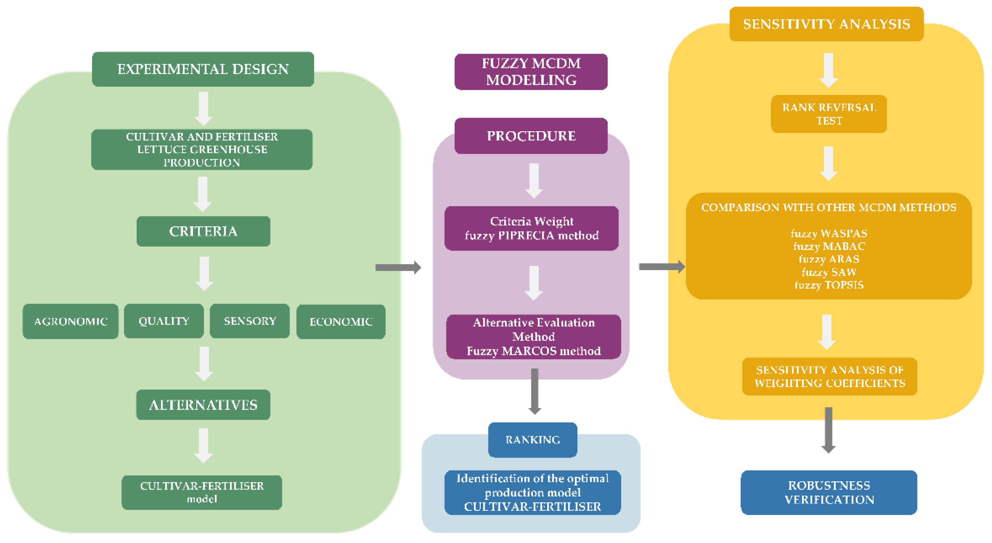
The research was carried out across two distinct phases, with their structure illustrated in Figure 1. Data on cultivars, fertilisers, and parameters from this study serve as inputs to the fuzzy model.

2.1. Experimental Design and Data Collection

2.1.1. Plant Material and Microbiological Fertilisers

Three lettuce cultivars (Lactuca sativa var. crispa ‘Carmesi’; Lactuca sativa var. capitata ‘Aquino’ and ‘Gaugin’) were evaluated in this study. Seeds were obtained from the official local distributor for the Rijk Zwaan company (De Lier, the Netherlands). Lettuce seeds were sown in 4 cm peat cubes (Potground H, Klasmann-Deilmann GmbH, Geeste, Germany) under glasshouse conditions (45°04′16.29″ N 19°51′27.54″ E; 159 m above sea level). After germination in the dark, seedlings were cultivated using irrigation only. Climatic data during the 20-day seedling production period included an average daily temperature of 18.1 °C and relative humidity of 61.1%. Lettuce transplants at the four-leaf unfolded stage were then planted in the greenhouse.
Two microbiological fertilisers were applied: EM Aktiv (Candor, EM Tehnologija d.o.o., Valpovo, Croatia), a liquid formulation produced through microbiological fermentation of organic matter and sugar cane molasses containing plant-derived extracts, and Vital Tricho (Candor, EM Tehnologija d.o.o., Valpovo, Croatia), a powder formulation containing two Trichoderma species (Trichoderma asperellum and Trichoderma viride; 5 × 10⁹ CFU mL−1). The third variant consisted of the combined application of EM Aktiv and Vital Tricho through their direct mixing before application.

2.1.2. Experimental Design

Plants were cultivated during the autumn growing period (October–December 2016) in an unheated 256 m2 greenhouse covered with single-layer plastic film (Ginegar Plastic Products Ltd., Kibbutz Ginegar, Israel) typical for moderately continental regions like Serbia (44°47′39″ N, 20°20′12″ E; 73 m above sea level). The plastic film was disinfected with Dioxy Activ Supra AGRO (ITR d.o.o., Sarajevo, Bosnia and Herzegovina) before transplanting plants into the greenhouse. Randomised soil samples were then collected from 0–30 cm depth for physical and chemical analyses before the experiment. Three composite soil samples, each consisting of multiple points collected via a zig-zag pattern across the greenhouse, were gathered. Initial soil analysis revealed black marsh soil that was organic matter-rich (5.02%), a clay loam characterised by a mildly alkaline pH of 7.8, medium levels of total nitrogen (0.22%), and high levels of readily available phosphorus (58.35 mg 10−2 g−1) and potassium (32.45 mg 10−2 g−1). Thus, only microbial fertilisers were applied to assess their effects, and the soil was prepared with a tractor and tiller, marked, treated, and covered with black mulch film. The experiment was organised in a complete block design following four treatments: (a) control (excluding any type of fertilisation), (b) application of EM Aktiv fertiliser, (c) application of Vital Tricho fertiliser, and (d) application of combined fertilisers EM Aktiv and Vital Tricho. It included three replicate plots per treatment, each with 32 plants in 2 × 1 m plots (transplanting density of 25 × 25 cm, 50 cm between replicates, and 100 cm between treatments). Fertilisers were soil-applied: 150 mL EM Aktiv, 21 g Vital Tricho, and a combination of 150 mL + 21 g of EM Aktiv + Vital Tricho, respectively, each dissolved in 10 L of water. Foliar applications included 30 mL EM Aktiv, 12 g Vital Tricho, and 30 mL + 12 g of EM Aktiv + Vital Tricho, each dissolved in 6 L of water, applied four times during the vegetation period using a battery sprayer.

2.1.3. Cultivation and Climatic Data

Agricultural practices for greenhouse lettuce production were followed, including irrigation, ventilation, hoeing, weeding, and preventive pest and disease control. Irrigation was applied based on soil physical characteristics, plant needs, and climatic data using overhead NaanDanJain 501-U sprinklers (Jain Irrigation Systems Ltd., Jalgaon, India) eight times during the vegetation period. Greenhouse ventilation was conducted daily by opening doors according to external temperature and air humidity to prevent excessive moisture accumulation. Hoeing and manual weeding were performed once per growing cycle to control weeds. Preventive disease protection used copper(II) hydroxide (Everest, Chemical Agrosava, Belgrade, Serbia) at 0.3% concentration. Lettuce plants were hand-harvested at marketable size and physiological maturity, 58 days after transplanting. Climatic conditions were recorded continuously over 24 h periods using an RC-4HC data logger (Elitech Technology Inc., San Jose, CA, USA), which recorded average day/night temperatures of 11.9/5.7 °C (maximum/minimum 17.3/−1.8 °C), average relative humidity of 87.2%, and a short photoperiod ranging from 11 to 9 h during the growing cycle.

2.1.4. Structure of the Decision Problem: Alternatives and Criteria

Twelve cultivar–fertiliser combinations (Table 1) were established for decision-making analysis.
Alternatives A1–A3 represent control variants, in which the cultivars ‘Aquino’, ‘Carmesi’, and ‘Gaugin’ were grown without microbiological fertiliser. Alternatives A4–A6 assessed the effects of EM Aktiv fertiliser on these three cultivars, whereas A7–A9 evaluated those of Vital Tricho fertiliser. Alternatives A10–A12 examined the combined influence of these two biofertilisers on the same cultivars. Ten criteria were evaluated for each alternative, as detailed in Table 2.

2.1.5. Data Collection and Measurement Protocols

Soil Analysis Protocols
Soil pH was measured potentiometrically using a SevenCompact S210-K pH meter (Mettler-Toledo, Greifensee, Switzerland) [46]. Total nitrogen and total carbon were determined by dry combustion on a Vario EL III CNS elemental analyser (Elementar, Hanau, Germany) [47,48]. Available phosphorus was quantified colourimetrically with a UV-160A spectrophotometer (Shimadzu, Kyoto, Japan), and available potassium by flame emission photometry (HINOTEK FP6440, Ningbo, China), both using the ammonium lactate method [49]. Carbonate content (CaCO3) was determined volumetrically [50]. Soil organic matter was estimated from total carbon after carbonate correction using the standard Van Bemmelen conversion factor of 1.724 [51].
Criteria Measurement Protocols
The core ratio (C1)—a unitless parameter defined as the ratio of stem length to rosette height [29]—was calculated following ruler measurements of stem length (cm) and rosette height (cm). The number of leaves (C2) was counted during the measurement of yield and other morphological parameters.
Fresh leaves were then packed in plastic bags and stored at −20 °C for analyses of antioxidant activity, total soluble solids, and chlorogenic acid content. For nitrate analysis, fresh leaves were oven-dried at 70 °C for 72 h to a constant weight and the dried samples were further used.
Nitrate content in lettuce leaves (C3) was determined using the rapid colourimetric method based on salicylic acid nitration [52], with sulfamic acid added to remove nitrite [53]. Absorbance was measured at 410–420 nm, and results were expressed as mg kg−1 FW.
Lettuce tissue was homogenised, extracted with 80% ethanol, and centrifuged at 10.000× g for 10 min. The supernatant was used for total antioxidant capacity (C4) analysis, measured according to Miller et al. [54] and modified by Böhm et al. [55]. Ethanolic extracts and Trolox standards were used to generate a calibration curve, with absorbance recorded spectrophotometrically at 734 nm (UV-VIS spectrophotometer; Labomed, Inc., Los Angeles, CA, USA). Results were expressed as μmol Trolox equivalents g−1 FW.
Total soluble solids (C5) were measured at room temperature using a digital hand-held refractometer (VEE GEE Scientific, LLC, Vernon Hills, IL, USA) on leaf juice [56], with results expressed as degrees of Brix (°Brix).
Chlorogenic acid (C6) was quantified from frozen samples homogenised in 80% methanol acidified with formic acid (98:2, v/v) and analysed using a Waters HPLC system (Waters, Milford, MA, USA) [32]. Peaks were recorded LC/MS/ESI in negative ion mode (m/z 100–900), validated and quantified with Empower 2 software (Waters, Milford, MA, USA) via the external standard method. Results are expressed as milligrams per gram of dry weight (mg g−1 DW).
On harvest day, a sensory panel of four trained panellists—who underwent training based on ISO 8586 guidelines for selecting, training, and monitoring assessors [57]—evaluated lettuce taste by identifying and ranking bitterness, sweetness, saltiness, and sourness using five graded solutions (water as control). Samples were prepared beforehand by removing damaged or discoloured outer leaves, washing, drying, and presenting in coded portions for each treatment in plastic bags, with water and toasted bread provided for palate cleansing. Overall taste was rated on a 5-point hedonic scale (1 = very poor; 5 = very good) as described by Ponce et al. [58], where lower scores were primarily linked to bitter taste, which negatively impacted perceptions.
Overall lettuce quality (C8) was assessed one day before harvest by trained evaluators in the greenhouse using a 1–5 scale. They received prior instruction on evaluating traits—colour, defects (from disease, pests, or physiological disorders), and marketability—adapted from Ansorena et al. [59] using the original 9-point scale. Scores were assigned as follows: 1 = poor/unmarketable (extensive discoloration, major defects, or decay); 3 = fair/marketable (minor defects or moderate colour changes); 5 = excellent (fully acceptable appearance, no yellowing, browning, defects, or decay); overall quality was calculated as the average of these three trait scores.
Total variable costs (C9) included materials (seeds/seedlings, agrochemicals, microbiological fertilisers, black mulch film, and others), energy, labour, sales packaging, and other costs, calculated over the vegetation period (October–December 2016). Each cost component was obtained by multiplying the quantity used by the average local market price for the specified input in the year the experiment was conducted, sourced from regional agricultural suppliers in Belgrade, Serbia. All measures that required electricity and fuel, such as irrigation and tractor preparation of the soil, were also calculated. Fuel costs for soil preparation were calculated based on litres of fuel used, while electricity costs for the electrical pump were determined by multiplying total working hours by the electricity rate per hour. Workers’ labour costs were determined by multiplying the required labour hours per production process by the average wage rate in the given year. Sales packaging costs included the price of one carton box and a plastic bag per 12 lettuce heads. Differences in the values of individual variable cost elements arose from the specifics of the production technology applied in each alternative. For example, in alternatives without the use of biofertilisers, these costs were 0.00 EUR, while in other variants, differences in their market prices directly caused variations in input costs. Similarly, total labour engagement costs varied among alternatives for the same reason; alternatives that did not include the application of biofertilisers achieved the lowest labour expenditure.
Total income (C10) was determined by multiplying harvested yield (fresh rosette weight per m2) by the average sales price per cultivar. Total variable costs and total income are expressed in EUR per m2 for all tested alternatives.

2.2. Multi-Criteria Decision-Making (MCDM) Modelling and Statistical Analysis

2.2.1. Operations with Fuzzy Numbers

Fuzzy numbers represent a concept that enables quantification of data uncertainty and imprecision (vagueness). Triangular fuzzy numbers (TFNs), the most prevalent type, are defined as A ~ = ( l , m , u ) , where l and u are the lower and upper limits, and m is the modal value.
The membership function of TFN-a is expressed with the following equation:
μ A ~ x = x l m l , l x m u x u m , m x u 0 , otherwise
Basic operations on triangular fuzzy numbers (TFNs), such as addition, subtraction, multiplication, and division, are performed directly on their triples (l, m, u), enabling simple calculations and applications in various MCDM methods [60].

2.2.2. The Fuzzy Pivot Pairwise Relative Criteria Importance Assessment (Fuzzy PIPRECIA) Method

This method for determining weight coefficients using fuzzy numbers was developed by Stević et al. [60]. The method consists of 11 steps, detailed below. In the first step, the decision-making team is selected, along with the criteria for comparison and their ordering; their relative importance need not be considered at this stage. In the second step, starting from the second criterion, each criterion is compared pairwise with the preceding one using importance comparison tables (Table 3), and a matrix ( s j ¯ ) is formed by computing the geometric mean of all decision-maker evaluations for the criteria.
The next step involves determining the coefficient ( k j ¯ ) by applying the equation:
k j ¯ = = 1 ¯ if j = 1 2 s j ¯ if j > 1
In the fourth step, the fuzzy weights ( q j ¯ ) are determined using the equation:
q j ¯ = = 1 ¯ if j = 1 q j 1 ¯ k j ¯ if j > 1
Then, in the next step, the relative weights of the criteria ( w j ¯ ) are derived using the given formula:
w j ¯ = q j ¯ j = 1 n q j ¯
In steps 6–9, the inverse fuzzy PIPRECIA methodology is applied by reversing the criterion order (from last to first) and repeating the prior steps. In the tenth step, final weighting coefficients for each criterion are obtained as the average of the defuzzified relative weights ( w j ¯ ) and ( w j ¯ ) (obtained in steps 5 and 9), and the final value of the weighting coefficients for each criterion ( w j ) is determined using the designated formula:
w j = w j + w j 2
In the eleventh step, results are validated using Pearson’s and Spearman’s correlation coefficients to assess consistency between fuzzy PIPRECIA and inverse fuzzy PIPRECIA weighting coefficients, or their ranks.

2.2.3. The Fuzzy Measurement Alternatives and Ranking According to COmpromise Solution (Fuzzy MARCOS) Method

The fuzzy MARCOS method for ranking alternatives was developed by Stanković et al. [61] and is implemented through 10 steps. In the first step, an initial fuzzy decision matrix is formed, with alternatives evaluated using the linguistic scale provided in Table 4.
The initial matrix is expanded in the second step by adding the fuzzy ideal ( A ~ ID ) and the fuzzy anti-ideal alternative ( A ~ AI ) .
  C ~ 1 C ~ 2 C ~ n X ~ = A ~ A I A ~ 1 A ~ 2 A ~ m A ~ I D x ~ a i 1 x ~ a i 2 x ~ a i n x ~ 11 x ~ 12 x ~ 1 n x ~ 21 x ~ 22 x ~ 2 n x ~ m 1 x ~ m 2 x ~ m n x ~ i d 1 x ~ i d 2 x ~ i d n
In the third step, data from the expanded matrix are normalised to form a normalised fuzzy matrix ( n ~ i j ), with cost-type criteria transformed using the following formula:
n ~ i j = n i j l , n i j m , n i j u = x i d l x i j u , x i d l x i j m , x i d l x i j l
While the benefit criteria for normalisation use the formula:
n ~ i j = n i j l , n i j m , n i j u = x i j l x i d u , x i j m x i d u , x i j u x i d u
In the next step, a computation of the weighted fuzzy matrix V ~ is formed by multiplying the elements of the normalised fuzzy matrix ( N ~ ) with fuzzy weight coefficients ( w ~ j ), that is:
v i j = v i j l , v i j m , v i j u = n ~ i j w ~ j = n i j l × w j l , n i j m × w j m , n i j u × w j u
In the next step, the ( S ~ i ) matrix is formed by applying the formula:
S ~ i = i = 1 n v ~ i j
The degree of usefulness of the alternatives is determined yielding the ( K ~ i ) and ( K ~ i + ) matrices via the following formulas:
K ~ i = S ~ i S ~ a i = s i l s a i u , s i m s a i m , s i u s a i l
K ~ i + = S ~ i S ~ i d = s i l s i d u , s i m s i d m , s i u s i d l
In the next step, the degrees of usefulness for the alternatives are aggregated, forming the fuzzy matrix ( T ~ i ) using the following formula:
T ~ i = t ~ i = ( t i l , t i m , t i u ) = K ~ i K ~ i + = ( k i l + k i + l , k i m + k i + m , k i u + k i + u )
In the same step, based on the elements of the matrix ( T ~ i ) , the fuzzy number D ~ i is determined using the formula:
D ~ i = d l , d m , d u max i t ~ i j
Then, it is necessary to defuzzify the number ( D ~ i ) by applying the expression ( d f c r i s p ) (defuzzified crisp value), where:
d f c r i s p = l + 4 m + u 6
In the eighth step, the utility function of the alternatives is determined in relation to the ideal ( f K ~ i + ) and anti-ideal ( f K ~ i ) solution, applying the following equations:
f K ~ i + = K ~ i d f c r i s p = k i l d f c r i s p , k i m d f c r i s p , k i u d f c r i s p
f K ~ i = K ~ i + d f c r i s p = k i + l d f c r i s p , k i + m d f c r i s p , k i + u d f c r i s p
Also, in the same step, after determining the utility functions of alternatives, it is necessary to defuzzify ( K ~ i ) , ( K ~ i + ) , f K ~ i , and f K ~ i + values by applying the form used for defuzzification of the number ( D ~ i ) .
The final defuzzified utility function of each alternative ( f K i ) is determined by applying the formula:
f K i = K i + + K i 1 + 1 f K i + f K i + + 1 f K i f K i
In the final step, alternatives are ranked based on their utility function values, with higher values being preferable and vice versa.

2.2.4. Methodology of Sensitivity Analysis

The sensitivity analysis procedure was carried out in three phases. Given that one of the main disadvantages of applying MCDM methods is the change in the ranking list when adding or removing alternatives [62,63], a Rank reversal test was conducted in the first phase through 10 scenarios. In the first scenario, the worst alternative was removed, and a ranking procedure was carried out; the same procedure was repeated across the remaining scenarios, up to scenario 10, in which two alternatives remained. In the second phase, the ranking results of alternatives using the fuzzy MARCOS method were compared with five other MCDM methods: fuzzy WASPAS (fuzzy Weighted Aggregated Sum Product Assessment method with fuzzy values [64]), fuzzy MABAC (fuzzy Multi-Attributive Border Approximation Area Comparison [65]), fuzzy ARAS (fuzzy Additive Ratio Assessment [66]), fuzzy SAW (fuzzy Simple Additive Weighting [67]), and fuzzy TOPSIS (fuzzy Technique for Order Performance by Similarity to Ideal Solution [68]). In the third phase, the influence of changes in weighting coefficients on the ranking results of alternatives was examined using the fuzzy MARCOS method through 20 scenarios: in each of the first 10 scenarios, one criterion was assigned 30% more importance while the others remained unchanged; in the next 10 scenarios, one criterion was reduced in importance by 30% while the others remained unchanged.
The proposed framework integrates fuzzy PIPRECIA for determining criteria weights with the fuzzy MARCOS method for ranking cultivar–fertiliser alternatives. Unlike conventional studies that rely on a limited set of economic or agronomic indicators, this research incorporates four distinct groups of criteria, enabling a comprehensive agro-economic evaluation under uncertainty.

2.2.5. Statistical Analysis

Statistical analyses of quantity, quality, and sensory parameters included two-way ANOVA to assess the main effects of cultivar and biofertiliser, as well as their interaction. Pearson’s correlation coefficient evaluated relationships among these parameters (criteria). Significance was set at α = 0.05. All analyses were performed using SPSS Statistics (Version 25.0; IBM Corp., Armonk, NY, USA) and Microsoft Excel 2019 (Microsoft Corp., Redmond, WA, USA). ANOVA results (F-value and significance level) are reported in the results tables for completeness and transparency, but are not further analysed, as the primary focus of this study is the fuzzy logic method and selection of the optimal cultivar–fertiliser model over single-parameter evaluation.

3. Results

3.1. ANOVA and Correlation Analysis

Two-way ANOVA results (Table 5) showed that cultivar significantly affected all criteria. Biofertiliser significantly influenced AOX, overall quality, and yield. Significant cultivar × biofertiliser interactions were detected for core ratio, AOX, chlorogenic acid, overall taste, and yield.
Pearson correlation coefficients are presented in Table 6. Yield, the most important quantity criterion, showed strong positive correlations with the number of leaves (0.72 **), overall quality (0.62 **), and nitrate content (0.63 **). Increasing yield was associated with a higher number of leaves, overall quality, and nitrate content.
AOX exhibited a very strong positive correlation with chlorogenic acid (0.86 **) and a weak positive correlation with overall quality (0.35 *), but a strong negative correlation with TSS (−0.67 **), and a moderate negative correlation with overall taste (−0.49 **).
Overall taste, an important sensory criterion, showed moderate positive correlation with TSS (0.43 **), and moderate negative correlations with AOX (−0.49 **) and chlorogenic acid (−0.48 **).
Correlation analysis revealed contrasting relationships between criteria that highlight the need for multi-criteria optimisation. Key trends included higher yields expected to correlate with elevated nitrate content, alongside taste deterioration from increased chlorogenic acid and antioxidant activity. These trade-offs underscore the value of fuzzy logic MCDM to identify optimal cultivar–biofertiliser combinations balancing all criteria simultaneously.
Economic criteria were analysed separately due to their distinct calculation methods, excluding them from the two-way ANOVA and Pearson correlation analyses. Yield—used to calculate total income—was included in the ANOVA testing.

3.2. Structure of Variable Costs

The ninth criterion for selecting the most favourable alternative is the structure of variable costs, which varies by lettuce cultivar and is summarised in Table 7.
Key factors driving differences in total variable costs include variations in fertilisation, seeds/seedlings, and labour across lettuce cultivars and fertilisation methods. Seedling costs—which encompass seed prices and transplant growth in peat cubes—form the largest share of material costs for all examined cultivars. Material costs form the biggest portion of total variable costs, followed by packaging, with other costs the smallest. The ‘Carmesi’ cultivar showed the lowest seedling (and thus overall variable) costs, whereas ‘Gaugin’ had the highest in both.

3.3. Determination of the Weighting Coefficients of the Criteria Using the Fuzzy PIPRECIA Method

A team of four decision-making experts determined the weighting coefficients. These included three professors from the Faculty of Agriculture (specialising in agroeconomics, vegetable production, and plant physiology) and one PhD holder from the ready-to-eat salad industry with 7 years of practical experience. The initial comparison tables for the criteria selected in this study (steps 2 and 6) are presented in Table 8. Full calculation of the initial criteria comparison for all criteria is given in Supplementary Table S1.
The mean values ( s j ¯ ) of decision-makers’ responses on pairwise comparisons of selected criteria—obtained using the aforementioned scales—were calculated via geometric mean. Subsequently, the coefficient ( k j ¯ ) , fuzzy weights ( q j ¯ ), and relative criterion weights ( w j ¯ ) were determined for both process phases, as presented in Table 9.
Based on the defuzzified values in the final column of the previous table, the final weighting coefficient values are determined (Table 10).
For the obtained weight values from the fuzzy PIPRECIA and inverse fuzzy PIPRECIA methods (Table 10), the correlation coefficient values were greater than 0.80, indicating that the ranking is largely consistent.

3.4. Ranking of Alternatives Using the Fuzzy MARCOS Method

Using a linguistic scale for evaluating alternatives (Table 4), the initial decision matrix—with linguistic assessments of each alternative’s criteria—is presented in Table 11.
Linguistic values were replaced with fuzzy numbers, and in the next step, the extended fuzzy matrix was formed (Table 12).
In the third step, a normalised matrix was formed, where criteria C1, C3, and C9 were normalised using the formula for cost criteria, while for the others, the procedure involved normalisation using the formula for benefit criteria. For the purpose of forming the weighted matrix, the final fuzzy weights of the criteria were determined by aggregating the values obtained from the PIPRECIA and PIPRECIA-I methods, as presented in Table 13. Fuzzy weights for all criteria are presented in Supplementary Table S2.
By multiplying the values of the fuzzy weight coefficients by the values of the normalised matrix, a fuzzy weighted normalised matrix was formed (Table 14). Fuzzy weighted normalised decision matrix calculation for all criteria is presented in Supplementary Table S3.
In the next step, the sums of the weighted values were formed for all alternatives ( S ~ i ), and then the degrees of utility of the alternatives relative to the anti-ideal and ideal alternative were determined— K ~ i K ~ i + matrices. Subsequently, the degrees of utility of the alternatives were summed, and a fuzzy matrix was formed T ~ i , and a fuzzy number was determined D ~ i , which was then defuzzified, and finally, the value of d f c r i s p was established (Table 15).
Based on the calculated d f c r i s p values from the previous table, the utility functions of the alternatives relative to the ideal and anti-ideal solutions were determined ( f K ~ i f K ~ i + ), and then the degrees of utility of the alternatives ( K ~ i , K ~ i + ) as well as the utility functions were defuzzified. In the final step, the final defuzzified utility function for each alternative was determined, based on which the ranking was performed (Table 16).
The results obtained from applying the integrated fuzzy PIPRECIA and fuzzy MARCOS method clearly indicate the superior performance of certain alternatives in the evaluation process. Specifically, alternative A11 emerged as the best-ranked alternative, corresponding to the ‘Aguino’ cultivar grown in a production system utilising the combined application of both fertilisers (Table 16). The second-ranked alternative was A6, which involved the ‘Carmesi’ cultivar treated solely with EM Aktiv, and the third-ranked alternative was A7, featuring the ‘Aguino’ cultivar amended with Vital Tricho. In contrast, the lowest-ranked alternative was A10, representing the ‘Gaugin’ cultivar with application of the combined fertilisers.

3.5. Sensitivity Analysis and Validation of Results

3.5.1. Rank Reversal Test

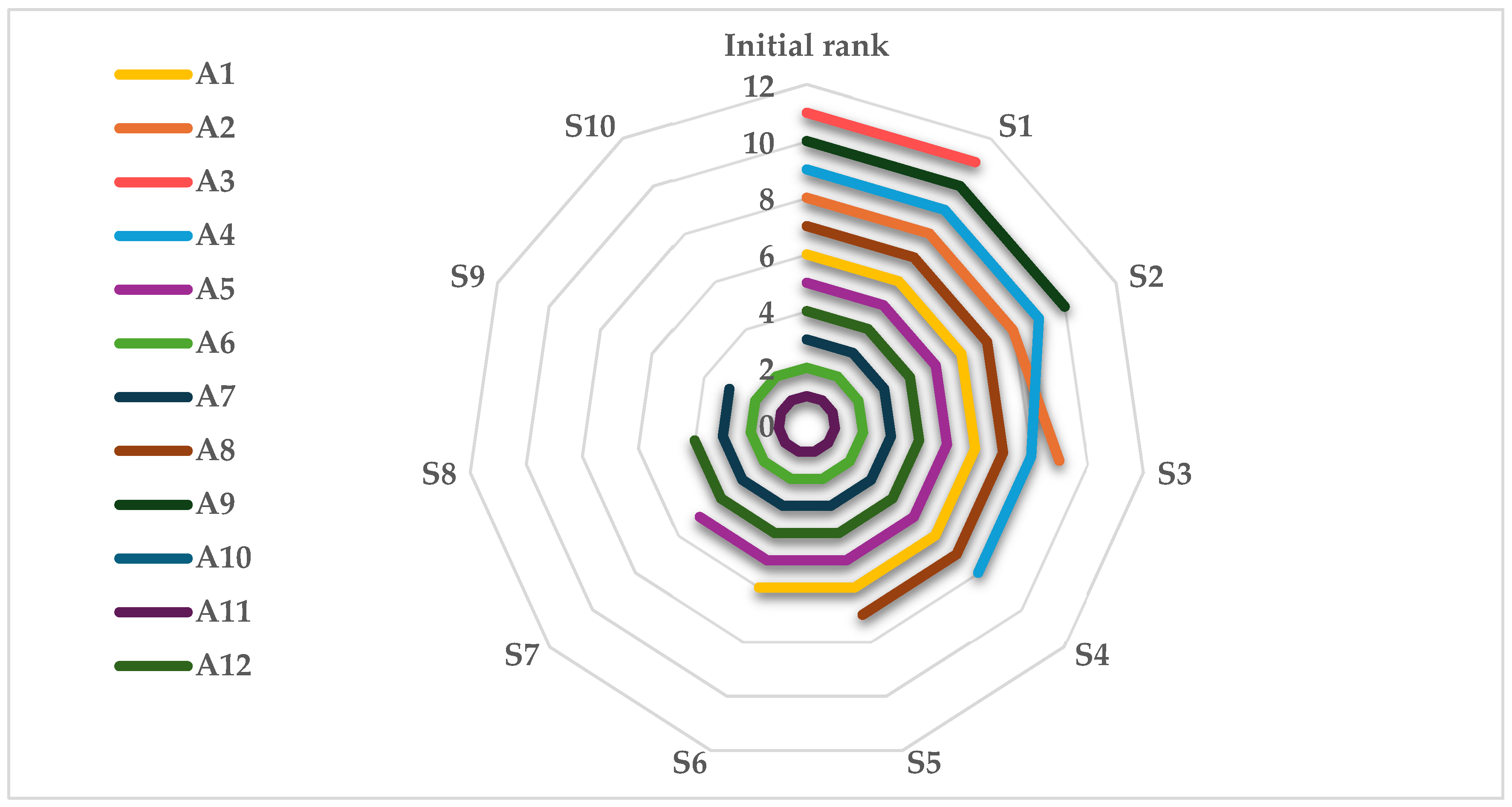
Given that the ranking results of the selected alternatives using the fuzzy MARCOS method indicate that alternative A10 was ranked as the worst in the first scenario (S1) of the Rank reversal test, it was removed, and the ranking of the remaining alternatives was conducted using the same method. In the second scenario (S2), the worst-ranked alternative from the first scenario (A3) was removed, and the ranking procedure was repeated. The remaining eight scenarios (S3–S10) were conducted in the same manner. The results are presented in Figure 2.
Results from Figure 2 indicate that alternatives A2 and A4, which were initially ranked in the eighth and ninth positions, swap positions in one scenario, while all other alternatives maintain the same ranking positions across all scenarios.

3.5.2. Comparison with Other Fuzzy MCDM Methods

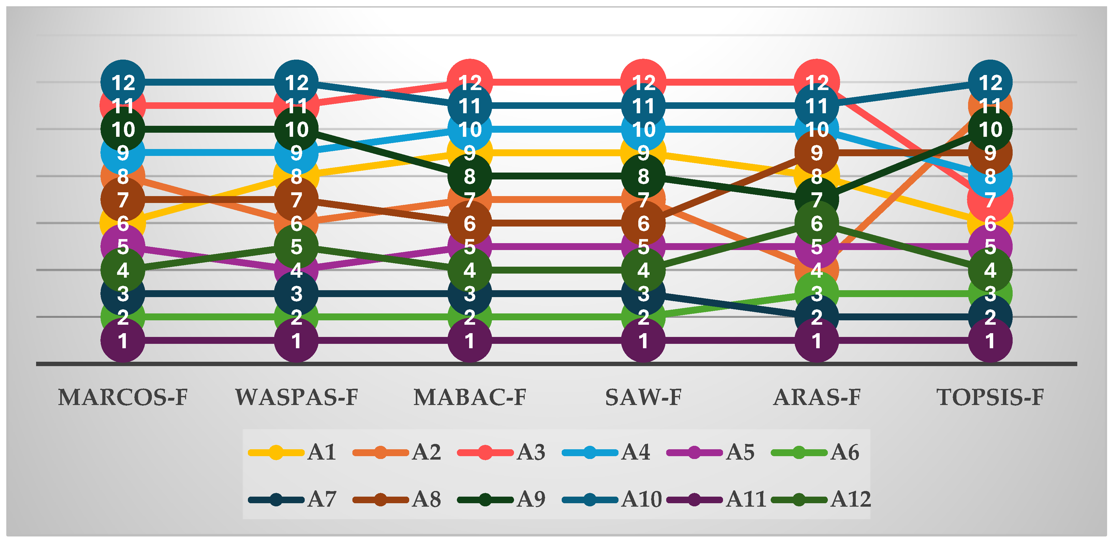
The results of comparing the rankings of the observed alternatives using the fuzzy MARCOS method with the other mentioned MCDM methods are given in Figure 3. These results demonstrate that different fuzzy MCDM methods produce consistent ranking orders across alternatives.

3.5.3. Sensitivity Analysis of Criteria Weights

In the third phase of sensitivity analysis, the effect of weight coefficient changes on alternative rankings was examined across 20 scenarios, as shown in Figure 4.
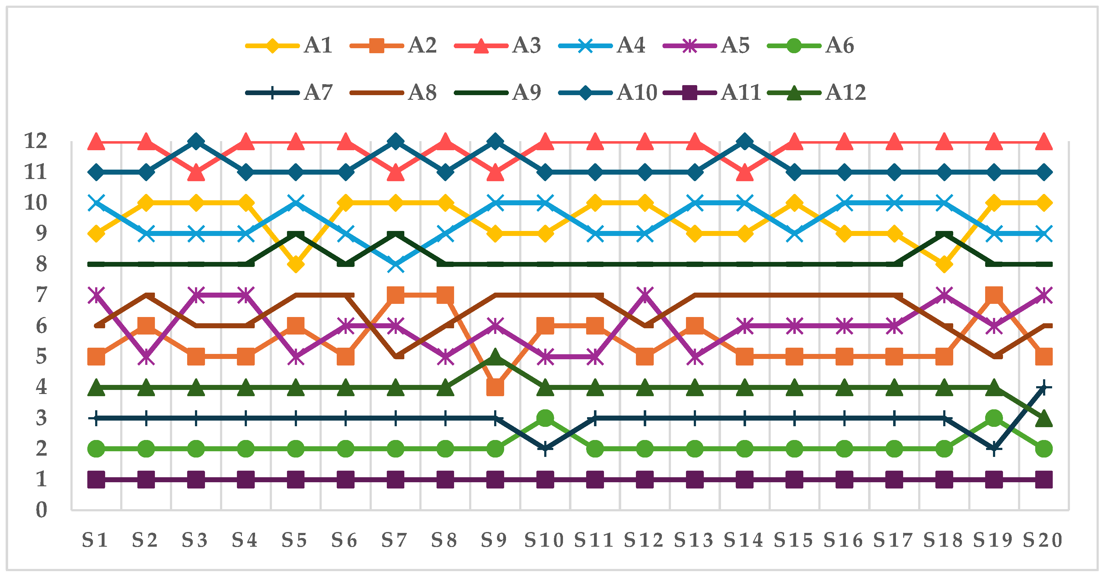
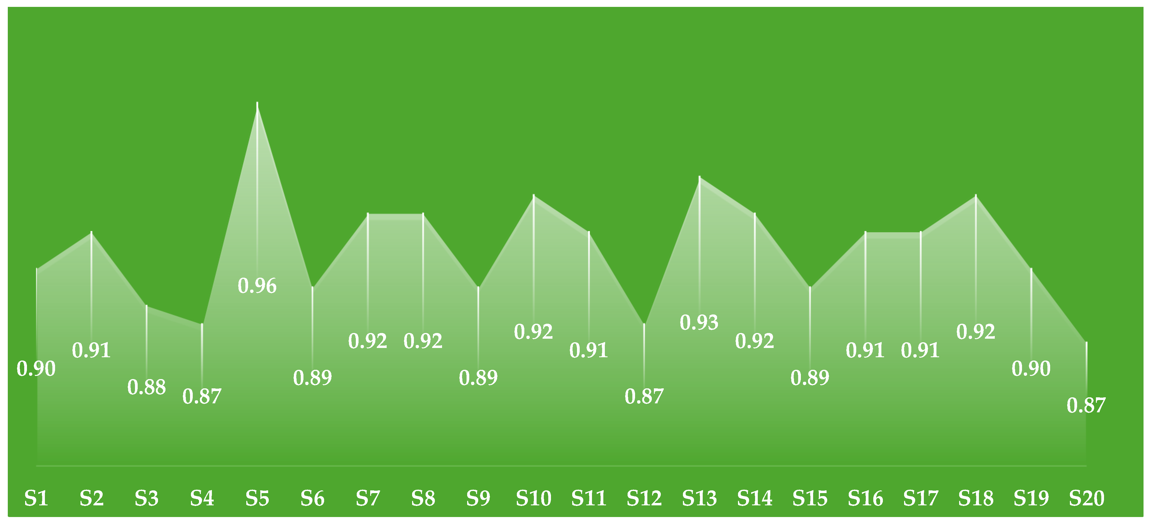
Results in Figure 4 clearly indicate that the alternative rankings do not change significantly across scenarios, with the best alternative retaining the first position in all scenarios, while the alternatives ranked in the next three positions remain the same in 18 out of 20 scenarios. The Spearman rank correlation coefficient between the initial ranking list and the ranking lists in the aforementioned 20 scenarios averaged 0.90, ranging from 0.87 to 0.96 (Figure 5).

4. Discussion

Growers and the processing industry face new demands every year for production quantities, quality, safety, and marketability. Product quality is as crucial as yield for all production sectors. Quality standard checks often decline during lettuce shortages—such as those caused by extreme disease and pest outbreaks or adverse environmental conditions—while they are carefully examined during surpluses [69].
ANOVA results showed statistically significant effects of cultivar on quantity, quality, and sensory criteria (Table 5). Optimal fresh weight plays a pivotal role in marketability and processing efficiency, directly influencing quality and profitability. However, findings on biofertilisers’ impact on plant productivity remain inconsistent—some studies report positive effects, such as increased fresh weight in lettuce, while others observe limited or no benefits. For instance, combining humic biostimulants with microbial inocula improved lettuce fresh weight compared to the control [70]. Similarly, plant growth-promoting rhizobacteria increased lettuce head fresh weight and leaf number under field conditions [26]. Applications of Trichoderma asperellum strains (TaMFP1, TaMFP2) and Trichoderma harzianum also boosted lettuce fresh leaf weight [71]. These outcomes likely stem from microorganisms producing hormones, vitamins, enzymes, and plant growth-promoting compounds that enhance nutrient availability, uptake, and overall plant growth. Yet, their efficacy varies by plant species, soil type, soil fertility, application method, and frequency. Likewise, Trichoderma performance depends on cultivar, the strain’s root colonisation ability, and application method [72]. Like plants, microorganisms have specific environmental demands and limitations tied to production methods [73].
Leaf number is influenced by agrotechnical practices and environmental factors; for example, high temperatures can accelerate the vegetative phase, causing premature flowering and a reduced number of leaves [74]. A similar trend appears in butterhead lettuce, where positive correlations existed between plant fresh weight and other morphological parameters under varying photoperiods and light intensities [75]. Longer internal stem length was linked to inferior quality in crisphead lettuce [76], which is consistent with our moderate negative correlation between core ratio and total soluble solids (Table 6). Nitrogen accumulation varies by lettuce type and cultivar, with seasonality significantly affecting nitrate levels—particularly during short days and low light when nitrate reductase activity decreases [77]. Fresh weight and nitrate content showed no significant correlation with application of nanohydroxyapatite/hydrogel/N-fertilisers [78]. In contrast, our study found positive correlations between yield and nitrate levels (Table 6), with higher yields linked to higher nitrate content.
The literature highlights clear distinctions between green and red lettuce cultivars: green types typically exhibit higher head weight, while red show greater antioxidant capacity [79,80]. Application of a bacterial–algal preparation in romaine lettuce increased total antioxidant capacity 2.5-fold during the summer season compared to controls [81]. Along with genotype, environmental factors—such as suboptimal conditions—can enhance TAC to counter oxidative stress in lettuce [82]. Although fertilisers did not affect chlorogenic acid content, interaction between cultivar and biofertiliser had significant effect in lettuce [32], aligning with our findings (Table 5). Apart from genotype, polyphenol content in lettuce is influenced by growing treatments that alter nutrient availability; for example, a quarter-strength reduced-nutrient solution increased polyphenol accumulation compared to a full-strength solution [83]. Abiotic stress conditions activate the phenylpropanoid biosynthetic pathway, boosting various phenolic compounds that improve plant performance under stress.
Taste is a key trait for breeders, producers, and consumers. Lettuce taste depends on sugars (sweetness) versus organic acids, phenolics, and sesquiterpene lactones (bitterness). Overall taste showed negative correlations with AOX and chlorogenic acid (Table 6), indicating that higher levels of these compounds—particularly chlorogenic acid—likely contribute to bitterness or astringency, thereby reducing taste palatability.
Cultivar and biofertiliser effects create complex trade-offs across yield, taste, nitrate content, AOX, and production costs, complicating decisions about optimal cultivar–biofertiliser combinations for farmers, processors, and consumers. Contrasting correlation coefficients between yield and nitrate, AOX and overall taste, and chlorogenic acid and overall taste—along with significant cultivar × treatment interactions for core ratio, AOX, chlorogenic acid, overall taste, and yield—demonstrate that our fuzzy MCDM framework provides the optimal solution for selecting the best cultivar–biofertiliser combinations in lettuce production.
Beyond market pressures, costs for land, labour, fuel, nutrient inputs, packaging, safety, and transport are escalating. This requires global cost reductions in lettuce production. Our study showed that seedling costs represent the largest share of material costs, which dominate total variable costs for all cultivars, followed by packaging, while other costs have the smallest share (Table 7). Variable costs account for 73.96% of total production costs in lettuce greenhouse production, as shown in a Turkish case study [84]. Similarly, seeds and growing media represent the highest variable costs in hydroponic lettuce production [85].
To address heating—one of the major costs—growers avoid energy use for heating, employ alternative coverings for frost protection, or favour frost-tolerant crops like lettuce during cold periods [86]. Still, surging energy prices have made greenhouse lettuce too costly [87]. For example, in regions with water scarcity, rising fertiliser costs are prompting farmers to adopt new practices for better resource efficiency and improved crop productivity [88]. Unheated greenhouses are a good option for lettuce in continental climates, avoiding additional heating costs and allowing for other material costs to dominate. Individual growers and food processing companies must consider not only agronomic factors, but also overall production costs and returns. Beyond infrastructure, production costs primarily arise from inputs, enabling effective reductions through simple changes in cultivation management [89]. The literature data show that vegetable production in unheated greenhouses is economically viable under different investment models [90].
Research on lettuce and escarole production in Spain showed that higher greenhouse yields did not justify the environmental impact, recommending nitrogen fertiliser optimisation as the most effective path to cleaner production [91]. There has been a global shift toward organic production, with consumers prioritising sustainability over large sizes and ideal shape [92]. The conversion to integrated farming considers lower inputs of fertilisers, pesticides, and improved soil management practices that can address economic and ecological challenges [93]. In recent years, the focus has been on developing new technologies to improve lettuce production through greater efficiency, lower costs, and enhanced sustainability [94]. Thus, biofertilisers justify their application in lettuce production due to the possible harmful effects of large quantities of mineral fertilisers and pesticides, as well as their negative impact on the nitrate content and overall quality of produce.
The application of MCDM methods is essential for solving different problems in agriculture, as ANOVA suits only single criteria, while fuzzy approaches better capture human reasoning and qualitative data, such as sensory traits. In this context linguistic terms thus provide a more suitable representation of these traits.
The fuzzy MARCOS method offers several advantages: it considers fuzzy reference points (ideal and anti-ideal solutions) from the outset of model formation; it enables more precise utility degree determination; it introduces novel ways to define and aggregate utility functions; and it handles large sets of criteria and alternatives [61]. These authors confirmed its suitability for uncertain environments, yielding stable results in dynamic, data-rich environments. For these reasons, we selected fuzzy MARCOS to address unpredictable conditions in an unheated greenhouse, including interactions between lettuce cultivars and effective microorganisms. A similar rationale guided optimal rapeseed variety selection using fuzzy logic, fuzzy PIPRECIA–fuzzy MABAC model to account for unforeseen climatic conditions [95]. The weighting coefficients of the criteria, determined using the fuzzy PIPRECIA method, showed that the weight values obtained by the fuzzy PIPRECIA and inverse fuzzy PIPRECIA methods had correlation coefficients above 0.80, indicating a high degree of ranking consistency [96].
The fuzzy MARCOS method has been widely employed across agriculture: Puška et al. [97] used it for selecting sustainable suppliers based on economic, social, and environmental criteria; Maksimović et al. [98] for choosing plum varieties for new orchards; Abualkishik et al. [99] for evaluating smart agricultural production efficiency; Puška et al. [100] for enhancing sustainable agro-touristic offerings; Puška et al. [101] for ranking affordable drones suited to small and medium-sized farms; and Mondal et al. [102] for assessing sustainable forest resource management models using the Pythagorean fuzzy MEREC-MARCOS approach.
MCDM methods have primarily addressed fruit production challenges [41,103,104,105]. In contrast, vegetable production requires more intensive timing management: annual crops like lettuce provide multiple cycles per year, with vegetation periods ranging from 55 to 70 or 70 to 100 days [106] depending on the production system, lettuce type, and environmental conditions. Vegetable production creates faster revenue for producers compared to fruit production, making it logical to use MCDM methods for fast and reliable decision-making on optimal production solutions.
Rank reversal, a phenomenon in various MCDM methods, occurs when alternative rankings change upon adding/removing an uninformative alternative—yet methods prone to it remain widely used [107]. Results from the Rank reversal test indicate that, out of 10 analysed scenarios, the only change occurred in the third scenario. This involved a swap in the rank positions of alternatives A2 and A4 (ranked eighth and ninth), resulting in their rotation (Figure 2).
No significant changes were observed in the alternative ranking when applying different MCDM methods (Figure 3). We validated and compared these results using the fuzzy WASPAS, fuzzy SAW, fuzzy MABAC, fuzzy ARAS, and fuzzy TOPSIS. Each method has its own specifics and, therefore, was used to confirm the results obtained by the fuzzy MARCOS method. Due to these differences, it is necessary to examine the results from these methods and check whether they agree with those from the fuzzy MARCOS method. The best-ranked alternative (A11, Aguino—EM Aktiv + Vital Tricho) retained its position across all methods, while the lowest-ranked alternative (A10, Gaugin—EM Aktiv + Vital Tricho) remained stable, consistently placed last or second-to-last. Alternatives A6 and A7 maintained identical ranks (second and third) under fuzzy WASPAS, fuzzy MABAC, and fuzzy SAW, though they swapped positions under fuzzy ARAS and fuzzy TOPSIS. These greater oscillations in certain alternatives stem from their highly similar characteristics, as well as differences in normalisation procedures and the mathematical foundations of the methods. The fuzzy MARCOS method’s suitability is confirmed by similar results in plum variety selection using the same methods [98]. This analysis does not question the value of the results obtained with the fuzzy MARCOS method, which are confirmed by those from other methods. In this way, its application is justified because the results obtained by this method do not deviate from the results of similar methods.
Additionally, Spearman’s correlation coefficient between the fuzzy MARCOS and other MCDM approaches ranges from 0.85 to 0.99, indicating a high degree of ranking agreement. The strongest similarity was with fuzzy WASPAS (r = 0.99), and the weakest with fuzzy ARAS (r = 0.85). All values above 0.80 confirm the stable and reliable performance of fuzzy MARCOS relative to diverse MCDM methods, underscoring the model’s good robustness and limited sensitivity to changes in mathematical frameworks.
Similar conclusions emerge from the sensitivity analysis, which examined the impact of 20 scenarios involving ±30% changes in weight coefficients on ranking results. These variations caused no major deviations in alternative rankings. Alternative A11 retained the highest position across all scenarios (Figure 4). Alternatives A6, A7, and A12—ranked second, third, and fourth—held their positions in 90% of scenarios. In all scenarios, A3 and A10 ranked last or second-to-last. These findings highlight the method’s high stability and robustness, showing that selecting the most favourable alternatives remains independent of individual weight changes. In addition, the task of sensitivity analysis is not only to consider the impact of different criteria on the change in the value of alternatives, but also the impact of these changes on the overall ranking of alternatives [108]. Confirming our results, through sensitivity analysis, it has been shown that other fuzzy methods can be used, not only the fuzzy MARCOS method, similarly for apple selection using fuzzy methods [109].
Thus, the results from all three phases of the sensitivity analysis consistently demonstrate the high stability and robustness of the fuzzy MARCOS model. First, the Rank reversal test showed near-complete rank stability: across ten scenarios of alternative removal, only one rotation was recorded, with all other positions unchanged. Second, comparing fuzzy MARCOS with five other fuzzy MCDM methods revealed a high degree of agreement, with the best- and lowest-ranked alternatives remaining stable across all methods. Spearman’s coefficients between fuzzy MARCOS and the other approaches ranged from 0.85 to 0.99, confirming rank stability despite differences in normalisation and mathematical structures. The third phase—varying ten criteria by ±30% across 20 scenarios—further illustrates the model’s resilience to weight changes. Spearman’s rank correlation coefficients between the original ranking and those in the scenarios ranged from 0.87 to 0.96 (average 0.90) (Figure 5), indicating that weight variations did not disrupt the rank structure. Combined, the results of the Rank reversal test, method comparisons, and weight variation analysis confirm that the proposed fuzzy PIPRECIA–fuzzy MARCOS model exhibits high robustness, with key recommendations (especially selecting the most favourable alternative A11) that are stable and reliable across a wide range of decision conditions. Studies on lettuce show that combining bacterial and fungal genera improves agronomic traits [24,110,111], as confirmed in this study for the best-ranked alternative.
The complex interaction of various production factors, particularly in non-controlled agricultural environments, requires a comprehensive methodology for analysing factors jointly within a decision-making framework. In this context, the conjoint application of MCDM methods can provide a completely new insight into decision analysis by enabling the search for an optimal solution that simultaneously considers multiple criteria and ranks the best-performing alternatives. The evaluation of a limited number of cultivar-fertiliser combinations over a single growing season, alongside the Serbian market’s availability of over 20 cultivars and a similar number of microbial fertilisers (mostly imported from various seed and fertiliser companies), constitutes a study limitation.


5. Conclusions

MCDM methods showed clear differences in performance among the cultivar–fertiliser alternatives. Fuzzy PIPRECIA and fuzzy MARCOS identified alternative A11 (‘Aquino’ with combined biofertilisers) as the best choice. Sensitivity analysis over 20 scenarios using five additional methods validates ranking stability. The consistency across fuzzy MCDM methods confirms the reliability of the fuzzy PIPRECIA–fuzzy MARCOS framework for optimising sustainable agricultural practices.
Economic analysis indicates that optimising input costs, primarily seedling costs, is key to the model’s sustainability. These MCDM tools help select the optimal solutions to maintain crop performance and economic returns. On soils rich in organic matter and macronutrients, the framework supports an easy shift to sustainable practices by potentially decreasing mineral fertiliser use. This study extends fuzzy MARCOS applications to vegetable production planning.
Future research should examine more lettuce cultivars and biofertiliser combinations over multiple seasons to capture seasonal variability and develop robust guidelines. Farmer questionnaires can reveal key needs—such as disease resistance, yield stability, input costs, quality, safety, and market demands—linking research directly to practice. Advanced fuzzy MCDM methods with interval fuzzy sets or hesitant fuzzy linguistic terms could include these alongside sensory factors like taste and texture, making fuzzy MARCOS even more relevant to actual production and market dynamics.

Supplementary Materials

The following supporting information can be downloaded at: https://www.mdpi.com/article/10.3390/horticulturae12030368/s1, Table S1: Initial criteria comparison matrices for fuzzy PIPRECIA and inverse fuzzy PIPRECIA method; Table S2: Fuzzy weights of the criteria; Table S3: Fuzzy weighted normalised decision matrix.

Author Contributions

Conceptualisation, R.B. and M.S.; methodology, R.B., V.M. Đ.M., S.S. and M.S.; software, R.B.; M.M., V.M. and M.S.; validation, R.B., V.M., Đ.M., Z.J. and S.S.; formal analysis, R.B., M.M., V.M., S.S. and M.S.; investigation, R.B., Đ.M., Z.J., S.S. and M.S.; resources, R.B., V.M., Đ.M., Z.J. and M.S.; data curation, R.B., M.M., V.M. and M.S.; writing—original draft preparation, R.B. and M.S.; writing—review and editing, R.B., V.M., Đ.M., Z.J., S.S. and M.S.; visualisation, R.B. and M.S.; supervision, R.B. and Đ.M.; project administration, R.B., Đ.M., Z.J., S.S. and M.S.; funding acquisition, R.B., V.M., Đ.M., Z.J., S.S. and M.S. All authors have read and agreed to the published version of the manuscript.

Funding

This research was funded by the Ministry of Science, Technological Development, and Innovation of the Republic of Serbia under Contract No. 451-03-33/2026-03/200053, 451-03-33/2026-03/200010, and 451-03-34/2026-03/200116.

Data Availability Statement

The original contributions presented in this study are included in the article. Further inquiries can be directed to the corresponding authors.

Conflicts of Interest

The authors declare no conflicts of interest.

Abbreviations

The following abbreviations are used in this manuscript:
MCDMMulti-Criteria Decision-Making
PIPRECIAPIvot Pairwise RElative Criteria Importance Assessment
MARCOSMeasurement Alternatives and Ranking according to COmpromise Solution
FAOFood and Agriculture Organization of the United Nations
AOXTotal Antioxidant Capacity
AHPAnalytic Hierarchy Process
TOPSISTechnique for Order Performance by Similarity to Ideal Solution
ELECTREElimination and Choice Translating Reality
TFNTriangular Fuzzy Number
WASPASWeighted Aggregated Sum Product Assessment
MABACMulti-Attributive Border Approximation Area Comparison
ARASAdditive Ratio Assessment
SAWSimple Additive Weighting
UV-VISUltraviolet–Visible spectroscopy
HPLCHigh-Performance Liquid Chromatography
ESIElectrospray Ionisation
LC/MSLiquid Chromatography/Mass Spectrometry
EUREuro

References

  1. Pinotti, L.; Manoni, M.; Fumagalli, F.; Rovere, N.; Luciano, A.; Ottoboni, M.; Ferrari, L.; Cheli, F.; Djuragic, O. Reduce, Reuse, Recycle for Food Waste: A Second Life for Fresh-Cut Leafy Salad Crops in Animal Diets. Animals 2020, 10, 1082. [Google Scholar] [CrossRef] [PubMed]
  2. Rodrigues, J.P.B.; da Silveira, T.F.F.; Rodrigues, D.B.; Domínguez, L.; Morales, P.; Pires, T.C.S.P.; Oliveira, M.B.P.P.; Fernandes, Â.; Barros, L. Lactuca sativa L. Losses and Wastes as a Source of Biobased Ingredients. J. Sci. Food Agric. 2026, 106, 3577–3591. [Google Scholar] [CrossRef] [PubMed]
  3. Muttiah, R.S.; Thai, C.N.; Prussia, S.E.; Shewfelt, R.L.; Jordan, J.L. An Expert System for Lettuce Handling at a Retail Store. Trans. ASAE 1991, 31, 622–628. [Google Scholar] [CrossRef]
  4. Yang, X.A.-O.; Gil, M.A.-O.; Yang, Q.A.-O.; Tomás-Barberán, F.A.-O. Bioactive Compounds in Lettuce: Highlighting the Benefits to Human Health and Impacts of Preharvest and Postharvest Practices. Compr. Rev. Food Sci. Food Saf. 2022, 21, 4–45. [Google Scholar] [CrossRef] [PubMed]
  5. FAOSTAT. Food and Agriculture Organization of the United Nations Statistics Division. Available online: https://www.fao.org/faostat/en/#data/QCL (accessed on 19 January 2026).
  6. Živanović, M.; Mihajlović, M.; Jovanović, A.; Hrustić, J.; Vojvodić, M.; Pešić, B.; Bulajić, A. Sclerotinia Species Causing Lettuce Drop Disease in Serbia. Microorganisms 2026, 14, 189. [Google Scholar] [CrossRef]
  7. Aloryi, K.D.; Sandoya, G.V.; Begcy, K. Genome Landscape of the Universal Stress Protein Gene Family in Lettuce and Expression Profile in Response to Heat Stress. BMC Plant Biol. 2025, 25, 1636. [Google Scholar] [CrossRef]
  8. Petropoulou, A.S.; van Marrewijk, B.; de Zwart, F.; Elings, A.; Bijlaard, M.; van Daalen, T.; Jansen, G.; Hemming, S. Lettuce Production in Intelligent Greenhouses-3D Imaging and Computer Vision for Plant Spacing Decisions. Sensors 2023, 23, 2929. [Google Scholar] [CrossRef]
  9. Stanghellini, C. Horticultural production in greenhouses: Efficient use of water. Acta Hortic. 2014, 1034, 25–32. [Google Scholar] [CrossRef]
  10. Çerez, N.E.; Şahin, M. Effects of Irrigation Water Levels on Lettuce Yield and Water Use Efficiencies Under Unheated Greenhouse Conditions. Gesunde Pflanz. 2023, 75, 1315–1324. [Google Scholar] [CrossRef]
  11. Buyukcangaz, H. Deficit Irrigation Effects on Cabbage (Brassicaceae oleracea Var. capitata L. Grandslam F1) Yield in Unheated Greenhouse Condition. TURJAF 2018, 6, 1251–1257. [Google Scholar] [CrossRef][Green Version]
  12. Fajdetić, N.R.; Božić Ostojić, L.; Benković, R.; Zima, D.; Blažinkov, M.; Mirosavljević, K.; Popović, B.; Benković-Lačić, T. Effects of Three Organic Fertilizers and Biostimulants on the Morphological Traits and Secondary Metabolite Content of Lettuce. Horticulturae 2025, 11, 1288. [Google Scholar] [CrossRef]
  13. Li, X.; Shah, I.H.; Gong, X.; Azam, M.; Jinhui, W.; Li, P.; Zhang, Y.; Niu, Q.; Chang, L. Research on High-Accuracy, Lightweight, Superfast Model for Nitrogen Diagnosis and Plant Growth in Lettuce (Lactuca sativa L.). Horticulturae 2025, 11, 451. [Google Scholar] [CrossRef]
  14. Aydinsakir, K.; Karaca, C.; Ozkan, C.F.; Dinc, N.; Buyuktas, D.; Isik, M. Excess Nitrogen Exceeds the European Standards in Lettuce Grown under Greenhouse Conditions. Agron. J. 2019, 111, 764–769. [Google Scholar] [CrossRef]
  15. Zhang, X.; Zhang, L.; Liu, J.; Shen, Z.; Liu, Z.; Gu, H.; Hu, X.; Yu, Z.; Li, Y.; Jin, J.; et al. Biofertilizers Enhance Soil Fertility and Crop Yields through Microbial Community Modulation. Agronomy 2025, 15, 1572. [Google Scholar] [CrossRef]
  16. Le, T.Y.; Lee, J.; Shim, S.-Y.; Jung, J.; Kim, S.-R.; Hong, S.-H.; Lee, M.-G.; Hwang, S.-G. Effects of Liquid Bio-Fertilizer on Plant Growth, Antioxidant Activity, and Soil Bacterial Community During Cultivation of Chinese Cabbage (Brassica rapa L. ssp. pekinensis). Microorganisms 2025, 13, 1036. [Google Scholar] [CrossRef] [PubMed]
  17. Kudpeng, K.; Khoiri, A.N.; Duangfoo, T.; Cheevadhanarak, S.; Jirakkakul, J. Microbial–Organic Inputs with Glycine Supplementation Enhance Growth and Heat Stress Tolerance in Lettuce. Horticulturae 2025, 11, 935. [Google Scholar] [CrossRef]
  18. Di Mola, I.; Ottaiano, L.; Cozzolino, E.; Senatore, M.; Sacco, A.; El-Nakhel, C.; Rouphael, Y.; Mori, M. Trichoderma spp. And Mulching Films Differentially Boost Qualitative and Quantitative Aspects of Greenhouse Lettuce Under Diverse N Conditions. Horticulturae 2020, 6, 55. [Google Scholar] [CrossRef]
  19. Daniel, A.I.; Fadaka, A.O.; Gokul, A.; Bakare, O.O.; Aina, O.; Fisher, S.; Burt, A.F.; Mavumengwana, V.; Keyster, M.; Klein, A. Biofertilizer: The Future of Food Security and Food Safety. Microorganisms 2022, 10, 1220. [Google Scholar] [CrossRef]
  20. Abdullah, N.S.; Doni, F.; Mispan, M.S.; Saiman, M.Z.; Yusuf, Y.M.; Oke, M.A.; Suhaimi, N.S. Harnessing Trichoderma in Agriculture for Productivity and Sustainability. Agronomy 2021, 11, 2559. [Google Scholar] [CrossRef]
  21. Alzyoud, L.; Othman, Y.A.; Alananbeh, K.M.; Ayad, J.; Al-Amir, F.M. Influence of Trichoderma harzianum on Growth, Yield and Quality of Lettuce (Lactuca sativa) Grown under a Hydroponic System. Not. Bot. Horti Agrobot. 2025, 53, 14516. [Google Scholar] [CrossRef]
  22. Rouphael, Y.; Carillo, P.; Colla, G.; Fiorentino, N.; Sabatino, L.; El-Nakhel, C.; Giordano, M.; Pannico, A.; Cirillo, V.; Shabani, E.; et al. Appraisal of Combined Applications of Trichoderma Virens and a Biopolymer-Based Biostimulant on Lettuce Agronomical, Physiological, and Qualitative Properties under Variable N Regimes. Agronomy 2020, 10, 196. [Google Scholar] [CrossRef]
  23. Topolovec-Pintarić, S.; Stvorić, M.; Benko, B.; Slunjski, S.; Matočec, N.; Kušan, I. Assessing the Impact of a Novel Trichoderma sp. Strain Stp8 on Lettuce Yield and Mineral Content. J. Fungi 2025, 11, 743. [Google Scholar] [CrossRef]
  24. Moreira, V.d.A.; Oliveira, C.E.d.S.; Jalal, A.; Gato, I.M.B.; Oliveira, T.J.S.S.; Boleta, G.H.M.; Giolo, V.M.; Vitória, L.S.; Tamburi, K.V.; Filho, M.C.M.T. Inoculation with Trichoderma harzianum and Azospirillum brasilense Increases Nutrition and Yield of Hydroponic Lettuce. Arch. Microbiol. 2022, 204, 440. [Google Scholar] [CrossRef] [PubMed]
  25. Cuchca Ramos, S.; García, L.; Barboza, J.I.; Bustamante, D.E.; Calderon, M.S. Effects of Seaweed-Based Biostimulants on the Morphophysiological Profile of Lettuce (Lactuca sativa L.). Cogent Food Agric. 2025, 11, 2448594. [Google Scholar] [CrossRef]
  26. Tahiri, A.-i.; Raklami, A.; Bechtaoui, N.; Anli, M.; Boutasknit, A.; Oufdou, K.; Meddich, A. Beneficial Effects of Plant Growth Promoting Rhizobacteria, Arbuscular Mycorrhizal Fungi and Compost on Lettuce (Lactuca sativa) Growth under Field Conditions. Gesunde Pflanz. 2022, 74, 219–235. [Google Scholar] [CrossRef]
  27. Viacava, G.E.; Goyeneche, R.; Goñi, M.G.; Roura, S.I.; Agüero, M.V. Natural Elicitors as Preharvest Treatments to Improve Postharvest Quality of Butterhead Lettuce. Sci. Hortic. 2018, 228, 145–152. [Google Scholar] [CrossRef]
  28. Graciano, P.; Jacinto, A.; Silveira, A.; Castoldi, R.; Lima, T.; Charlo, H.; Silva, I.; Marin, M. Agronomic Biofortification with Zinc in Curly Lettuce Cultivars. Rev. Bras. Ciênc. Agrár. 2020, 15, 1–9. [Google Scholar] [CrossRef]
  29. Maboko, M.; Du Plooy, C. Evaluation of Crisphead Lettuce (Lactuca sativa L.) for Winter Production in a Soilless Production System. Afr. J. Plant Sci. 2008, 2, 113–117. [Google Scholar]
  30. Yahya, M.H.; Chadwick, M.; Wagstaff, C. Supplementary Light Intensity and Harvest Date Affect Midrib Oxidative Pinking and Related Metabolites in Two Romaine Lettuce Cultivars with Contrasting Discolouration Sensitivities. Horticulturae 2026, 12, 57. [Google Scholar] [CrossRef]
  31. Jiao, Y.; Yuan, X.; Ji, Y.; Xu, J.; Zhu, B.; Cui, J.; Cui, W.; Chen, Q.; Liang, B.; Zhou, W. Foliar Astaxanthin Application Effectively Reduces Nitrate Accumulation and Enhances Functional Traits in Hydroponically Grown Lettuce. Sci. Hortic. 2025, 339, 113881. [Google Scholar] [CrossRef]
  32. Stojanović, M.; Milosavljević, D.; Delcourt, A.; Hilbert, J.-L.; Hance, P.; Maksimović, V.; Dragišić Maksimović, J. Phytochemical Composition and Overall Taste Modulation in Lettuce: Combination of Cultivar and Biofertiliser. Plants 2025, 14, 3864. [Google Scholar] [CrossRef]
  33. Miao, M.; Xiang, L. Chapter Three–Pharmacological Action and Potential Targets of Chlorogenic Acid. In Advances in Pharmacology; Du, G., Ed.; Academic Press: Cambridge, MA, USA, 2020; Volume 87, pp. 71–88. [Google Scholar]
  34. Vargas-Arcila, M.; Cartagena-Valenzuela, J.R.; Franco, G.; Correa-Londoño, G.A.; Quintero-Vásquez, L.M.; Gaviria-Montoya, C.A. Changes in the Physico-Chemical Properties of Four Lettuce (Lactuca sativa L.) Varieties During Storage. Cienc. Tecnol. Agropecuaria 2017, 18, 257–273. [Google Scholar]
  35. Díaz-Pérez, M.; Cantón Ramos, J.M.; Velázquez Martí, B.; Callejón-Ferre, Á.-J. Commercial Quality of ‘Little Gem’ Lettuce Hearts. J. Agric. Food Res. 2024, 16, 101168. [Google Scholar] [CrossRef]
  36. Holmes, S.C.; Wells, D.E.; Pickens, J.M.; Kemble, J.M. Selection of Heat Tolerant Lettuce (Lactuca sativa L.) Cultivars Grown in Deep Water Culture and Their Marketability. Horticulturae 2019, 5, 50. [Google Scholar] [CrossRef]
  37. Zavadskas, E.K.; Turskis, Z. A New Additive Ratio Assessment (ARAS) Method in Multicriteria Decision-Making. Technol. Econ. Dev. Econ. 2010, 16, 159–172. [Google Scholar] [CrossRef]
  38. Taherdoost, H.; Madanchian, M. Multi-Criteria Decision Making (MCDM) Methods and Concepts. Encyclopedia 2023, 3, 77–87. [Google Scholar] [CrossRef]
  39. Cicciù, B.; Schramm, F.; Schramm, V.B. Multi-Criteria Decision Making/Aid Methods for Assessing Agricultural Sustainability: A Literature Review. Environ. Sci. Policy 2022, 138, 85–96. [Google Scholar] [CrossRef]
  40. Kumar, R. A Comprehensive Review of MCDM Methods, Applications, and Emerging Trends. Decis. Mak. Adv. 2024, 3, 185–199. [Google Scholar] [CrossRef]
  41. Nedeljković, M.; Puška, A.; Suzić, R.; Maksimović, A. Multicriteria Model of Support for the Selection of Pear Varieties in Raising Orchards in the Semberija Region (Bosnia and Herzegovina). Sustainability 2022, 14, 1584. [Google Scholar] [CrossRef]
  42. Erdoğdu, A.; Dayi, F.; Yildiz, F.; Yanik, A.; Ganji, F. Combining Fuzzy Logic and Genetic Algorithms to Optimize Cost, Time and Quality in Modern Agriculture. Sustainability 2025, 17, 2829. [Google Scholar] [CrossRef]
  43. Puška, A.; Kozarevic, S.; Stević, Ž.; Stovrag, J. A New Way of Applying Interval Fuzzy Logic in Group Decision Making for Supplier Selection. ECECSR 2018, 52, 217–234. [Google Scholar]
  44. Ferrari Putti, F.; Cremasco, C.P.; Neto, A.B.; Barbosa, A.C.; Júnior, J.F.; Reis, A.R.; Góes, B.C.; Arruda, B.; Filho, L.R. Fuzzy Modeling Development for Lettuce Plants Irrigated with Magnetically Treated Water. Plants 2023, 12, 3811. [Google Scholar] [CrossRef]
  45. Aisyah, P.Y.; Zarkasih, I.; Kurnia, M. Smart and Sustainable Hydroponics: Fuzzy Logic-Based Environmental Control for Optimized Indoor Crop Growth. Green Technol. Sustain. 2026, 4, 100311. [Google Scholar] [CrossRef]
  46. SRPS EN ISO 10390: 2022; Soil, Treated Biowaste and Sludge—Determination of pH. Institute for Standardisation of Republic of Serbia: Belgrade, Serbia, 2022. Available online: https://iss.rs/en/project/show/iss:proj:71952 (accessed on 26 February 2026).
  47. SRPS ISO 10694: 2005; Soil Quality—Determination of Organic and Total Carbon After Dry Combustion (Elementary Analysis). Institute for Standardisation of Republic of Serbia: Belgrade, Serbia, 2005. Available online: https://iss.rs/sr_Cyrl/project/show/iss:proj:17014 (accessed on 26 February 2026).
  48. SRPS ISO 13878: 2005; Soil Quality—Determination of Total Nitrogen Content by Dry Combustion (“Elemental Analysis”). Institute for Standardisation of Republic of Serbia: Belgrade, Serbia, 2005. Available online: https://iss.rs/sr_Cyrl/project/show/iss:proj:17429 (accessed on 26 February 2026).
  49. Latkovic, D.; Maksimovic, J.; Dinic, Z.; Pivic, R.; Stanojkovic, A.; Stanojkovic-Sebic, A. Case Study Upon Foliar Application of Biofertilizers Affecting Microbial Biomass and Enzyme Activity in Soil and Yield Related Properties of Maize and Wheat Grains. Biology 2020, 9, 452. [Google Scholar] [CrossRef]
  50. SRPS EN ISO 10693: 2005; Soil Quality—Determination of Carbonate Content—Volumetric Method. Institute for Standardisation of Republic of Serbia: Belgrade, Serbia, 2005. Available online: https://iss.rs/en/project/show/iss:proj:17363 (accessed on 26 February 2026).
  51. Nelson, D.W.; Sommers, L.E. Total Carbon, Organic Carbon, and Organic Matter. In Methods of Soil Analysis, Part 2, 2nd ed.; Page, A.L., Ed.; John Wiley & Sons: Madison, WI, USA, 1996; Volume 14, pp. 961–1010. [Google Scholar]
  52. Cataldo, D.A.; Maroon, M.; Schrader, L.E.; Youngs, V.L. Rapid Colorimetric Determination of Nitrate in Plant Tissue by Nitration of Salicylic Acid. Commun. Soil Sci. Plant Anal. 1975, 6, 71–80. [Google Scholar] [CrossRef]
  53. Jana, J.; Moktan, P. Nitrate Concentration of Leafy Vegetables: A Survey of Nitrite Concentrations in Retail Fresh Leafy Vegetables from Daily Markets of Different Locations. ISABB J. Food and Agric. Sci. 2013, 3, 1–5. [Google Scholar]
  54. Miller, N.J.; Sampson, J.; Candeias, L.P.; Bramley, P.M.; Rice-Evans, C.A. Antioxidant Activities of Carotenes and Xanthophylls. FEBS Lett. 1996, 384, 240–242. [Google Scholar] [CrossRef]
  55. Böhm, V.; Puspitasari-Nienaber, N.L.; Ferruzzi, M.G.; Schwartz, S.J. Trolox Equivalent Antioxidant Capacity of Different Geometrical Isomers of A-Carotene, Β-Carotene, Lycopene, and Zeaxanthin. J. Agric. Food Chem. 2002, 50, 221–226. [Google Scholar] [CrossRef]
  56. Ntsoane, L.L.M.; Soundy, P.; Jifon, J.; Sivakumar, D. Variety-Specific Responses of Lettuce Grown Under the Different-Coloured Shade Nets on Phytochemical Quality After Postharvest Storage. J. Hortic. Sci. Biotechnol. 2016, 91, 520–528. [Google Scholar] [CrossRef]
  57. ISO 8586:2023; Sensory Analysis—Selection and Training of Sensory Assessors. International Organization for Standardization: Geneva, Switzerland, 2023.
  58. Ponce, A.G.; Roura, S.; Moreira, M.D.R. Essential Oils as Biopreservatives: Different Methods for the Technological Application in Lettuce Leaves. J. Food Sci. 2011, 76, M34–M40. [Google Scholar] [CrossRef] [PubMed]
  59. Ansorena, M.R.; Goñi, M.G.; Aguëro, M.V.; Roura, S.I.; Di Scala, K.C. Application of the General Stability Index Method to Assess the Quality of Butter Lettuce During Postharvest Storage Using a Multi-Quality Indices Analysis. J. Food Eng. 2009, 92, 317–323. [Google Scholar] [CrossRef]
  60. Stević, Ž.; Stjepanović, Ž.; Božičković, Z.; Das, D.K.; Stanujkić, D. Assessment of Conditions for Implementing Information Technology in a Warehouse System: A Novel Fuzzy PIPRECIA Method. Symmetry 2018, 10, 586. [Google Scholar] [CrossRef]
  61. Stanković, M.; Stević, Ž.; Das, D.K.; Subotić, M.; Pamučar, D. A New Fuzzy MARCOS Method for Road Traffic Risk Analysis. Mathematics 2020, 8, 457. [Google Scholar] [CrossRef]
  62. Bakır, M.; Atalık, O. Application of Fuzzy AHP and Fuzzy MARCOS Approach for the Evaluation of E-Service Quality in the Airline Industry. Decis. Mak. Appl. Manag. Eng. 2021, 4, 127–152. [Google Scholar] [CrossRef]
  63. Yazdani, M.; Chatterjee, P.; Pamucar, D.; Abad, M.D. A Risk-Based Integrated Decision-Making Model for Green Supplier Selection: A Case Study of a Construction Company in Spain. Kybernetes 2019, 49, 1229–1252. [Google Scholar] [CrossRef]
  64. Turskis, Z.; Zavadskas, E.K.; Antuchevičienė, J.; Kosareva, N.J.I.J.C.C.C. A Hybrid Model Based on Fuzzy AHP and Fuzzy WASPAS for Construction Site Selection. Int. J. Comput. Commun. Control. 2015, 10, 113–128. [Google Scholar] [CrossRef]
  65. Bozanic, D.; Tešić, D.; Milićević, J. A Hybrid Fuzzy AHP-MABAC Model: Application in the Serbian Army—The Selection of the Location for Deep Wading as a Technique of Crossing the River by Tanks. Decis. Mak. Appl. Manag. Eng. 2018, 1, 143–164. [Google Scholar] [CrossRef]
  66. Nguyen, H.-T.; Md Dawal, S.Z.; Nukman, Y.; Rifai, P.A.; Aoyama, H. An Integrated MCDM Model for Conveyor Equipment Evaluation and Selection in an FMC Based on a Fuzzy AHP and Fuzzy ARAS in the Presence of Vagueness. PLoS ONE 2016, 11, e0153222. [Google Scholar] [CrossRef] [PubMed]
  67. Kabassi, K.; Karydis, C.; Botonis, A. AHP, Fuzzy SAW, and Fuzzy WPM for the Evaluation of Cultural Websites. Multimodal Technol. Interact. 2020, 4, 5. [Google Scholar] [CrossRef]
  68. Sun, C.-C. A Performance Evaluation Model by Integrating Fuzzy AHP and Fuzzy TOPSIS Methods. Expert Syst. Appl. 2010, 37, 7745–7754. [Google Scholar] [CrossRef]
  69. Simko, I.; Hayes, R.J.; Mou, B.; McCreight, J.D. Lettuce and Spinach. In Yield Gains in Major U.S. Field Crops; Smith, S., Diers, B., Specht, J., Carver, B., Eds.; CSSA Special Publications 33; Crop Science Society of America: Madison, WI, USA, 2014; pp. 53–85. [Google Scholar]
  70. Savarese, C.; Cozzolino, V.; Verrillo, M.; Vinci, G.; De Martino, A.; Scopa, A.; Piccolo, A. Combination of Humic Biostimulants with a Microbial Inoculum Improves Lettuce Productivity, Nutrient Uptake, and Primary and Secondary Metabolism. Plant Soil 2022, 481, 285–314. [Google Scholar] [CrossRef]
  71. Gutiérrez-Chávez, A.; Robles-Hernández, L.; Guerrero, B.I.; González-Franco, A.C.; Medina-Pérez, G.; Acevedo-Barrera, A.A.; Hernández-Huerta, J. Potential of Trichoderma asperellum as a Growth Promoter in Hydroponic Lettuce Cultivated in a Floating-Root System. Plants 2025, 14, 382. [Google Scholar] [CrossRef] [PubMed]
  72. López-Bucio, J.; Pelagio-Flores, R.; Herrera-Estrella, A. Trichoderma as Biostimulant: Exploiting the Multilevel Properties of a Plant Beneficial Fungus. Sci. Hortic. 2015, 196, 109–123. [Google Scholar] [CrossRef]
  73. Szczech, M.; Szafirowska, A.; Kowalczyk, W.; Szwejda-Grzybowska, J.; Włodarek, A.; Maciorowski, R. The Effect of Plant Growth Promoting Bacteria on Transplants Growth and Lettuce Yield in Organic Production. J. Hortic. Res. 2016, 24, 101–107. [Google Scholar] [CrossRef]
  74. Tobar-Tosse, D.E.; dos Santos Candido, W.; da Silva Santos, L.; Castoldi, R.; Costa Silva, E.H.; Trevisan Braz, L. Identifying Crisphead Lettuce Genotypes for a Wider Range of Environments. Cienc. Tecnol. Agropecu. 2022, 23, e1964. [Google Scholar] [CrossRef]
  75. Iqbal, Z.; Munir, M.; Sattar, M.N. Morphological, Biochemical, and Physiological Response of Butterhead Lettuce to Photo-Thermal Environments. Horticulturae 2022, 8, 515. [Google Scholar] [CrossRef]
  76. Maboko, M.M.; Ncayiyana, M.; Du Plooy, C.P. Evaluation of Butterhead Lettuce Cultivars for Winter Production under a Shadenet Structure. Acta Agric. Scand. Sect. B—Soil Plant Sci. 2015, 65, 177–181. [Google Scholar] [CrossRef]
  77. Govedarica-Lučić, A.; Perković, G. Effect of Variety and Production Methods on Nitrate Content in Lettuce. Agric. For. 2013, 14, 541–547. [Google Scholar] [CrossRef]
  78. Zyadeh, M.; Kasrawi, M.; Hamadneh, I.; Jaradat, S. The Effects of Novel Nanohydroxyapatite/Hydrogel/N-Fertilizers on the Growth and Quality of Lettuce. J. Saudi Soc. Agric. Sci. 2025, 24, 14. [Google Scholar] [CrossRef]
  79. Barickman, T.C.; Sublett, W.L.; Miles, C.A.; Crow, D.; Scheenstra, E. Lettuce Biomass Accumulation and Phytonutrient Concentrations Are Influenced by Genotype, N Application Rate and Location. Horticulturae 2018, 4, 12. [Google Scholar] [CrossRef]
  80. Liu, X.; Ardo, S.; Bunning, M.; Parry, J.; Zhou, K.; Stushnoff, C.; Stoniker, F.; Yu, L.; Kendall, P. Total Phenolic Content and Dpph Radical Scavenging Activity of Lettuce (Lactuca sativa L.) Grown in Colorado. LWT-Food Sci. Technol. 2007, 40, 552–557. [Google Scholar] [CrossRef]
  81. Kopta, T.; Pavlikova, M.; Sękara, A.; Pokluda, R.; Maršálek, B. Effect of Bacterial-Algal Biostimulant on the Yield and Internal Quality of Lettuce (Lactuca sativa L.) Produced for Spring and Summer Crop. Not. Bot. Horti Agrobot. 2018, 46, 615–621. [Google Scholar] [CrossRef]
  82. Pérez-López, U.; Miranda-Apodaca, J.; Muñoz-Rueda, A.; Mena-Petite, A. Interacting Effects of High Light and Elevated CO2 on the Nutraceutical Quality of Two Differently Pigmented Lactuca sativa Cultivars (Blonde of Paris Batavia and Oak Leaf). Sci. Hortic. 2015, 191, 38–48. [Google Scholar] [CrossRef]
  83. Senizza, B.; Zhang, L.; Miras-Moreno, B.; Righetti, L.; Zengin, G.; Ak, G.; Bruni, R.; Lucini, L.; Sifola, M.I.; El-Nakhel, C.; et al. The Strength of the Nutrient Solution Modulates the Functional Profile of Hydroponically Grown Lettuce in a Genotype-Dependent Manner. Foods 2020, 9, 1156. [Google Scholar] [CrossRef]
  84. Engindeniz, D.Y. Economic Analysis of Lettuce Growing in Greenhouse: A Case Study from Türkiye. J. Glob. Agric. Ecol. 2025, 17, 1–8. [Google Scholar] [CrossRef]
  85. Tarr, S.T.; Valle de Souza, S.; Lopez, R.G. Influence of Day and Night Temperature and Radiation Intensity on Growth, Quality, and Economics of Indoor Green Butterhead and Red Oakleaf Lettuce Production. Sustainability 2023, 15, 829. [Google Scholar] [CrossRef]
  86. Arin, L.; Şalk, A.; Deveci, M.; Polat, S. Kohlrabi Growing under Unheated Glasshouse Conditions in Turkey. Acta Agric. Scand. Sect. B Soil Plant Sci. 2003, 53, 38–41. [Google Scholar]
  87. Saget, S.; Styles, D.; Williams, M. Comparative Life Cycle Assessment of Alternative Winter Salad Value Chains Supplying the United Kingdom. Sci. Total Environ. 2024, 952, 175870. [Google Scholar] [CrossRef]
  88. Montazar, A.; Geisseler, D.; Cahn, M.D. Assessing Water and Nitrogen Management Practices in Drip-Irrigated Desert Lettuce. Horticulturae 2025, 11, 1507. [Google Scholar] [CrossRef]
  89. Vendruscolo, E.P.; Rodrigues, A.H.A.; Correia, S.R.; Oliveira, P.R.; Campos, L.F.C.; Seleguini, A. Economic Analysis of Crisp Lettuce Production in Different Planting Spacing and Soil Cover. Adv. Hortic. Sci. 2019, 33, 449–455. [Google Scholar]
  90. Bodiroga, R.; Sredojevic, Z.; Vico, G.; Govedarica-Lucic, A. Influence of Different Production Methods on Economic Results of Greenhouse Vegetable Production. Custos Agronegocio 2022, 18, 44–62. [Google Scholar]
  91. Romero-Gámez, M.; Audsley, E.; Suárez-Rey, E.M. Life Cycle Assessment of Cultivating Lettuce and Escarole in Spain. J. Clean. Prod. 2014, 73, 193–203. [Google Scholar] [CrossRef]
  92. Guzmán-Guzmán, P.; Kumar, A.; de los Santos-Villalobos, S.; Parra-Cota, F.I.; Orozco-Mosqueda, M.D.; Fadiji, A.E.; Hyder, S.; Babalola, O.O.; Santoyo, G. Trichoderma Species: Our Best Fungal Allies in the Biocontrol of Plant Diseases—A Review. Plants 2023, 12, 432. [Google Scholar] [CrossRef]
  93. Edwards, C.A. The Importance of Integration in Sustainable Agricultural Systems. Agr. Ecosyst. Environ. 1989, 27, 25–35. [Google Scholar] [CrossRef]
  94. Zaidi, A.; Ahmad, E.; Khan, M.; Saif, S.; Rizvi, A. Role of Plant Growth Promoting Rhizobacteria in Sustainable Production of Vegetables: Current Perspective. Sci. Hortic. 2015, 193, 231–239. [Google Scholar] [CrossRef]
  95. Nedeljković, M.; Puška, A.; Doljanica, S.; Virijević Jovanović, S.; Brzaković, P.; Stević, Ž.; Marinkovic, D. Evaluation of Rapeseed Varieties Using Novel Integrated Fuzzy PIPRECIA–Fuzzy MABAC Model. PLoS ONE 2021, 16, e0246857. [Google Scholar] [CrossRef] [PubMed]
  96. Bakır, M.; Akan, Ş.; Özdemir, E. Regional Aircraft Selection with Fuzzy PIPRECIA and Fuzzy MARCOS: A Case Study of the Turkish Airline Industry. Facta Univ. Ser. Mech. Eng. 2021, 19, 423. [Google Scholar] [CrossRef]
  97. Puška, A.; Stević, Ž.; Stojanović, I. Selection of Sustainable Suppliers Using the Fuzzy MARCOS Method. Curr. Chin. Sci. 2021, 1, 218–229. [Google Scholar] [CrossRef]
  98. Maksimović, A.; Puška, A.; Šakić Bobić, B.; Grgić, Z. A Model for Supporting the Decision of Plum Variety Selection Based on Fuzzy Logic. J. Cent. Eur. Agric. 2021, 22, 450–461. [Google Scholar] [CrossRef]
  99. Abualkishik, A.; Al-majed, R.; Thompson, W. Evaluating Smart Agricultural Production Efficiency Using Fuzzy MARCOS Method. J. Neutrosophic Fuzzy Syst. 2022, 3, 8–18. [Google Scholar] [CrossRef]
  100. Puška, A.; Nedeljkovic, M.; Jelocnik, M.; Subic, J.; Nancu, D.; Jean, A. An Assessment of Improving the Sustainable Agro-Touristic Offer in an Emerging Country Using the Integrative Approach Based on Fuzzy Logic. Front. Environ. Sci. 2022, 10, 894811. [Google Scholar] [CrossRef]
  101. Puška, A.; Nedeljković, M.; Štilić, A.; Božanić, D. Evaluation of Affordable Agricultural Drones for Small and Medium Farms. Eng 2024, 5, 3161–3173. [Google Scholar] [CrossRef]
  102. Mondal, M.K.; Mahapatra, B.S.; Bera, M.B.; Mahapatra, G.S. Sustainable Forest Resources Management Model through Pythagorean Fuzzy MEREC–MARCOS Approach. Environ. Dev. Sustain. 2024, 1–32. [Google Scholar] [CrossRef]
  103. Berk, P.; Stajnko, D.; Hočevar, M.; Malneršič, A.; Jejčič, V.; Belšak, A. Plant Protection Product Dose Rate Estimation in Apple Orchards Using a Fuzzy Logic System. PLoS ONE 2019, 14, e0214315. [Google Scholar] [CrossRef]
  104. Kin, T.; Abu Hasan, S.; Suraiya, S.S.d. Automated Mango Fruit Grading System Using Fuzzy Logic. J. Agric. Sci. 2013, 6, 41–47. [Google Scholar]
  105. Magalhães, B.; Gaspar, P.D.; Corceiro, A.; João, L.; Bumba, C. Fuzzy Logic Decision Support System to Predict Peaches Marketable Period at Highest Quality. Climate 2022, 10, 29. [Google Scholar] [CrossRef]
  106. Tudela, J.A.; Hernández, N.; Pérez-Vicente, A.; Gil, M.I. Growing Season Climates Affect Quality of Fresh-Cut Lettuce. Postharvest Biol. Technol. 2017, 123, 60–68. [Google Scholar] [CrossRef]
  107. Li, B.; Abbas, A. A Trend Analysis of Rank Reversal in Widely Used Decision-Making Methods. J. Multi-Criteria Decis. Anal. 2026, 33, e70027. [Google Scholar] [CrossRef]
  108. Puška, A.; Stojanović, I.; Maksimović, A. Evaluation of Sustainable Rural Tourism Potential in Brcko District of Bosnia and Herzegovina Using Multi-Criteria Analysis. Oper. Res. Eng. Sci. Theor. Appl. 2019, 2, 40–54. [Google Scholar] [CrossRef]
  109. Nedeljković, M.; Puška, A.; Maksimović, A.; Suzić, R. Selection of the Optimal Apple Variety for Raising Orchards Using the Methods of Multi-Criteria Analysis. Erwerbs-Obstbau 2023, 65, 201–214. [Google Scholar] [CrossRef]
  110. Rasouli, F.; Amini, T.; Asadi, M.; Hassanpouraghdam, M.B.; Aazami, M.A.; Ercisli, S.; Skrovankova, S.; Mlcek, J. Growth and Antioxidant Responses of Lettuce (Lactuca sativa L.) to Arbuscular Mycorrhiza Inoculation and Seaweed Extract Foliar Application. Agronomy 2022, 12, 401. [Google Scholar] [CrossRef]
  111. Oliveira, C.E.d.S.; Sena Oliveira, T.J.S.; Jalal, A.; Fernandes, G.C.; Bastos, A.d.C.; da Silva, M.R.; Sant’Ana, G.R.; Aguilar, J.V.; de Camargos, L.S.; Zoz, T.; et al. Inoculation and Co-Inoculation of Lettuce and Arugula Hydroponically Influence Nitrogen Metabolism, Plant Growth, Nutrient Acquisition and Photosynthesis. Front. Plant Sci. 2025, 16, 1547821. [Google Scholar] [CrossRef] [PubMed]
Figure 1. Structure of the multi-criteria decision-making process in choosing optimal lettuce production model.
Horticulturae 12 00368 g001
Figure 2. Rank reversal test. Alternatives abbreviations are provided under Table 1. S1: original ranking with worst alternative A10 removed; S2: S1 ranking with new worst A3 removed; S3–S10: iteratively remove each subsequent worst-ranked alternative from prior scenario.
Horticulturae 12 00368 g002
Figure 3. Ranking of alternatives using various fuzzy MCDM methods. Alternatives abbreviations are provided under Table 1.
Horticulturae 12 00368 g003
Figure 4. Impact of weight coefficient changes on MARCOS-F method ranking results. Alternatives abbreviations are provided under Table 1. Scenarios (S1–S20): S1–S10, each criterion assigned +30% importance (others unchanged); S11–S20, each criterion reduced −30% importance (others unchanged).
Horticulturae 12 00368 g004
Figure 5. Spearman rank correlation coefficient through different scenarios. Scenario (S1–S20) abbreviations are provided under Figure 4.
Horticulturae 12 00368 g005
Table 1. Lettuce production models.
Combination Cultivar–FertiliserModel (Alternative)
Aguino-controlAlternative 1 (A1)
Carmesi-controlAlternative 2 (A2)
Gaugin-controlAlternative 3 (A3)
Gaugin-EM AktivAlternative 4 (A4)
Aguino-EM AktivAlternative 5 (A5)
Carmesi-EM AktivAlternative 6 (A6)
Aguino-Vital TrichoAlternative 7 (A7)
Carmesi-Vital TrichoAlternative 8 (A8)
Gaugin-Vital TrichoAlternative 9 (A9)
Gaugin–EM Aktiv + Vital TrichoAlternative 10 (A10)
Aguino–EM Aktiv + Vital TrichoAlternative 11 (A11)
Carmesi–EM Aktiv + Vital TrichoAlternative 12 (A12)
Table 2. Criteria analysed in the study.
Criteria LabelCriteria Type
Quantitative criteria
C1Core ratio
C2Number of leaves
Qualitative criteria
C3Nitrate content
C4Total antioxidant capacity
C5Total soluble solids
C6Chlorogenic acid
Sensory criteria
C7Overall taste
C8Overall quality
Economic criteria
C9Total variable costs
C10Total income
Table 3. Scale for the assessment of criteria.
DFVlmuLinguistic Scale
1.0081.0001.0001.050Almost equal value
1.1501.1001.1501.200Slightly more significant
1.2921.2001.3001.350Moderately more significant
1.4331.3001.4501.500More significant
1.5751.4001.6001.650Much more significant
1.7171.5001.7501.800Dominantly more significant
1.8581.6001.9001.950Absolutely more significant
0.9440.6671.0001.000Weakly less significant
0.6940.5000.6671.000Moderately less significant
0.5110.4000.5000.667Less significant
0.4060.3330.4000.500Really less significant
0.3370.2860.3330.400Much less significant
0.2880.2500.2860.333Dominantly less significant
0.2510.2220.2500.286Absolutely less significant
1.0001.0001.0001.000Equal value
Source: Stević et al. [60]. Abbreviation: DFV: defuzzified value.
Table 4. A linguistic scale for evaluating alternatives.
Linguistic TermMarkTFN
Extremely poorEP111
Very poorVP113
PoorP133
Medium poorMP335
MediumM355
Medium goodMG557
GoodG577
Very goodVG779
Extremely goodEG799
Source: Stanković et al. [61].
Table 5. Two-way ANOVA of cultivar and biofertiliser effects on quantity, quality, and sensory criteria.
NLCRAOXTSSNITCGAOTOQY
FactorsF-ValueSig.F-ValueSig.F-ValueSig.F-ValueSig.F-ValueSig.F-ValueSig.F-ValueSig.F-ValueSig.F-ValueSig.
Cultivar (C)49.9***27.7***40.0***36.8***30.8***63.3***13.9***4.6*160.5***
Treatment (T)0.57ns1.7ns5.6**0.3ns0.1ns2.5ns1.2ns11.2***20.8***
C × T0.67ns4.8**3.7**1.0ns2.4ns2.6*4.1**0.6ns2.5*
Asterisks indicate significant differences at * p ≤ 0.05; ** p ≤ 0.01; *** p ≤ 0.001; ns: non-significant. Abbreviations: Sig.: significance; NL: number of leaves; CR: core ratio; AOX: total antioxidant capacity; TSS: total soluble solids; NIT: nitrate content; CGA: chlorogenic acid; OT: overall taste; OQ: overall quality; Y: yield.
Table 6. Pearson correlation coefficients among quantity, quality, and sensory criteria.
NLCRAOXTSSNITCGAOTOQY
NL1
CR0.53 **1
AOX−0.030.271
TSS0.11−0.53 **−0.67 **1
NIT0.81 **0.28−0.050.34 *1
CGA0.040.50 **0.86 **−0.77 **0.011
OT0.23−0.06−0.49 **0.43 **0.19−0.48 **1
OQ0.45 **0.100.35 *−0.020.290.220.081
Y0.72 **0.02−0.20.40 *0.63 **−0.280.33 *0.62 **1
** Correlation is significant at the 0.01 level (2-tailed). * Correlation is significant at the 0.05 level (2-tailed). Abbreviations: NL: number of leaves; CR: core ratio; AOX: total antioxidant capacity; TSS: total soluble solids; NIT: nitrate content; CGA: chlorogenic acid; OT: overall taste; OQ: overall quality; Y: yield.
Table 7. Variable costs structure in different lettuce cultivars.
No.Indicator (Cost Type)Cultivar (EUR per m2)
AguinoCarmesiGaugin
1.Material costs1.040–1.3760.902–1.2391.046–1.382
-Seedlings0.8100.6730.816
-Microbiological fertilisers0.000–0.3370.000–0.3370.000–0.337
-Agrochemicals0.0090.0090.009
-Black mulch film0.0520.0520.052
-Sprinklers for irrigation0.1680.1680.168
2.Costs of energy (fuel + electricity)0.0240.0240.024
3.Labour costs0.089–0.1150.089–0.1150.089–0.115
4.Cost of sales (packaging)0.3710.3710.371
5.Other costs0.0030.0030.003
6.Total variable costs1.526–1.8891.389–1.7521.532–1.895
Table 8. Initial criteria comparison matrices for fuzzy PIPRECIA and inverse fuzzy PIPRECIA method.
PIPRC1C2C3C4C5C10
DM1 (0.400,0.500,0.667)(1.400,1.600,1.650)(1.000,1.000,1.000)(0.667,1.000,1.000)(1.300,1.450,1.500)
DM2 (1.100,1.150,1.200)(1.500,1.750,1.800)(1.300,1.450,1.500)(0.400,0.500,0.667)(1.100,1.150,1.200)
DM3 (1.000,1.000,1.000)(1.400,1.600,1.650)(1.000,1.000,1.000)(0.400,0.500,0.667)(1.000,1.000,1.000)
DM4 (0.400,0.500,0.667)(1.500,1.750,1.800)(1.000,1.000,1.000)(0.667,1.000,1.000)(1.100,1.150,1.200)
PIPR-IC10C9C8C7C6C1
DM1 (0.333,0.400,0.500)(1.100,1.150,1.200)(1.000,1.000,1.000)(0.333,0.400,0.500)(1.200,1.300,1.350)
DM2 (0.667,1.000,1.000)(1.000,1.000,1.000)(1.000,1.000,1.000)(0.667,1.000,1.000)(0.667,1.000,1.000)
DM3 (1.000,1.000,1.000)(1.000,1.000,1.000)(1.000,1.000,1.000)(1.000,1.000,1.000)(1.000,1.000,1.000)
DM4 (0.667,1.000,1.000)(1.000,1.000,1.000)(1.000,1.000,1.000)(0.333,0.400,0.500)(1.200,1.300,1.350)
Criteria abbreviations are provided under Table 2. PIPR: fuzzy PIPRECIA; PIPR-I: inverse fuzzy PIPRECIA; DM: decision-maker response.
Table 9. Procedure for calculating relative criterion weights.
PIPRECIA s j ¯ k j ¯ q j ¯ w j ¯ DF
C1 1.0001.0001.0001.0001.0001.0000.0320.0500.1030.056
C20.6480.7320.8551.1451.2681.3520.7390.7890.8730.0240.0390.0900.045
C31.4491.6731.7230.2770.3270.5511.3422.4153.1570.0440.1200.3260.142
C41.0681.0971.1070.8930.9030.9321.4402.6753.5340.0470.1330.3650.157
C50.5170.7070.8171.1831.2931.4830.9712.0692.9860.0320.1030.3080.125
C60.7070.8290.9741.0261.1711.2930.7511.7662.9110.0240.0880.3000.113
C71.1401.2041.2400.7600.7960.8600.8732.2193.8290.0280.1110.3950.144
C81.0001.0001.0001.0001.0001.0000.8732.2193.8290.0280.1110.3950.144
C90.9041.0001.0001.0001.0001.0960.7962.2193.8290.0260.1110.3950.144
C101.1201.1771.2120.7880.8230.8800.9052.6964.8620.0290.1340.5020.178
Sum 9.69120.06730.810
PIPRECIA-I s j ¯ k j ¯ q j ¯ w j ¯ DF
C10.9901.1401.1620.8380.8601.0100.1910.3380.4870.0260.0530.0930.055
C20.2670.3090.3651.6351.6911.7330.1930.2900.4080.0260.0450.0780.048
C30.7600.7950.8411.1591.2051.2400.3350.4910.6680.0460.0770.1280.080
C41.0951.1401.1910.8090.8600.9050.4150.5910.7740.0570.0920.1480.096
C50.6620.7620.8831.1171.2381.3380.3750.5090.6270.0510.0790.1200.082
C60.5210.6320.7071.2931.3681.4790.5020.6290.7000.0680.0980.1340.099
C71.0001.0001.0001.0001.0001.0000.7430.8610.9050.1010.1340.1730.135
C81.0241.0361.0470.9530.9640.9760.7430.8610.9050.1010.1340.1730.135
C90.6200.7950.8411.1591.2051.3800.7250.8300.8630.0990.1300.1650.130
C10 1.0001.0001.0001.0001.0001.0000.1360.1560.1910.159
Sum 5.2226.4007.337
Abbreviations: s j ¯ : mean value of decision-makers’ response; k j ¯ : coefficient; q j ¯ : fuzzy weights; w j ¯ : relative criterion weights; DF: defuzzified crisp value. Criteria abbreviations are provided under Table 2.
Table 10. Final defuzzified weighting coefficient values.
Criteria LabelC1C2C3C4C5C6C7C8C9C10
Weight coefficient (Wi)0.0550.0460.1110.1270.1030.1060.1400.1400.1370.168
Abbreviations: Wi: weight coefficient. Criteria abbreviations are provided under Table 2.
Table 11. Initial decision matrix—linguistic ratings.
Alternative LabelLinguistic Values of Criteria
C1C2C3C4C5C6C7C8C9C10
A1PPVGMPVGEPMPMPPP
A2EPEPMPMPMGEPPPEPEP
A3MPVPMPMPVPVPPMGPEP
A4MPMMEPVPMGMPVP
A5PMPGPGEPMPVGMPMP
A6VPEPMPPVGEPMMGVPEP
A7PMPGPVGEPMGVGVGM
A8VPEPMPMPGEPMGMGMGEP
A9PPMGVGEPPEPEGVGVP
A10PPMGGMPVPEPVGVGVP
A11PMGPVGEPGEGVGMG
A12VPEPMPMPVGEPMVGMGVP
Alternatives abbreviations are provided under Table 1. Criteria abbreviations are provided under Table 2. Linguistic values of criteria abbreviations: EP: extremely poor; VP: very poor; P: poor; MP: medium poor; M: medium; MG: medium good; G: good; VG: very good; EG: extremely good.
Table 12. Extended initial fuzzy matrix.
AC1C2C3C4C5C6C7C8C9C10
AAI(3,5,5)(1,1,1)(7,7,9)(1,3,3)(1,1,1)(1,1,1)(1,1,1)(1,3,3)(7,7,9)(1,1,1)
A1(1,3,3)(1,3,3)(7,7,9)(3,3,5)(7,7,9)(1,1,1)(3,3,5)(3,3,5)(1,3,3)(1,3,3)
A2(1,1,1)(1,1,1)(3,3,5)(3,3,5)(5,5,7)(1,1,1)(1,3,3)(1,3,3)(1,1,1)(1,1,1)
A3(3,3,5)(1,1,3)(3,3,5)(3,3,5)(1,1,3)(1,1,3)(1,3,3)(5,5,7)(1,3,3)(1,1,1)
A4(3,5,5)(1,3,3)(3,5,5)(3,5,5)(1,1,1)(1,1,3)(3,5,5)(5,7,7)(3,3,5)(1,1,3)
A5(1,3,3)(3,3,5)(5,7,7)(1,3,3)(5,7,7)(1,1,1)(3,3,5)(7,7,9)(3,3,5)(3,3,5)
A6(1,1,3)(1,1,1)(3,3,5)(1,3,3)(7,7,9)(1,1,1)(3,5,5)(5,5,7)(1,1,3)(1,1,1)
A7(1,3,3)(3,3,5)(5,7,7)(1,3,3)(7,7,9)(1,1,1)(5,5,7)(7,7,9)(7,7,9)(3,5,5)
A8(1,1,3)(1,1,1)(3,3,5)(3,3,5)(5,7,7)(1,1,1)(5,5,7)(5,5,7)(5,5,7)(1,1,1)
A9(1,3,3)(1,3,3)(5,5,7)(7,7,9)(1,1,1)(1,3,3)(1,1,1)(7,9,9)(7,7,9)(1,1,3)
A10(1,3,3)(1,3,3)(5,5,7)(5,7,7)(3,3,5)(1,1,3)(1,1,1)(7,7,9)(7,7,9)(1,1,3)
A11(1,3,3)(3,5,5)(5,7,7)(1,3,3)(7,7,9)(1,1,1)(5,7,7)(7,9,9)(7,7,9)(5,5,7)
A12(1,1,3)(1,1,1)(3,3,5)(3,3,5)(7,7,9)(1,1,1)(3,5,5)(7,7,9)(5,5,7)(1,1,3)
AI(1,1,1)(3,5,5)(3,3,5)(7,7,9)(7,7,9)(1,3,3)(5,7,7)(7,9,9)(1,1,1)(5,5,7)
Abbreviations: AI: ideal alternatives; AAI: anti-ideal alternatives. Criteria abbreviations provided under Table 2. Alternatives abbreviations are provided under Table 1.
Table 13. Fuzzy weights of the criteria.
CC1C2C3C4C10
wi(0.029,0.051,0.098)(0.025,0.042,0.084)(0.045,0.099,0.227)(0.052,0.113,0.256)(0.083,0.145,0.347)
Abbreviations: wi: fuzzy weights. Criteria abbreviations are provided under Table 2.
Table 14. Fuzzy weighted normalised decision matrix.
AC1C2C3C4C5C10
AAI(0.006,0.010,0.033)(0.005,0.008,0.017)(0.015,0.042,0.097)(0.006,0.038,0.085)(0.005,0.010,0.024)(0.012,0.021,0.050)
A1(0.010,0.017,0.098)(0.005,0.025,0.050)(0.015,0.042,0.097)(0.017,0.038,0.142)(0.032,0.071,0.214)(0.012,0.062,0.149)
A2(0.029,0.051,0.098)(0.005,0.008,0.017)(0.027,0.099,0.227)(0.017,0.038,0.142)(0.023,0.051,0.166)(0.012,0.021,0.050)
A3(0.006,0.017,0.033)(0.005,0.008,0.050)(0.027,0.099,0.227)(0.017,0.038,0.142)(0.005,0.010,0.071)(0.012,0.021,0.050)
A4(0.006,0.010,0.033)(0.005,0.025,0.050)(0.027,0.059,0.227)(0.017,0.063,0.142)(0.005,0.010,0.024)(0.012,0.021,0.149)
A5(0.010,0.017,0.098)(0.015,0.025,0.084)(0.019,0.042,0.136)(0.006,0.038,0.085)(0.023,0.071,0.166)(0.035,0.062,0.248)
A6(0.010,0.051,0.098)(0.005,0.008,0.017)(0.027,0.099,0.227)(0.006,0.038,0.085)(0.032,0.071,0.214)(0.012,0.021,0.050)
A7(0.010,0.017,0.098)(0.015,0.025,0.084)(0.019,0.042,0.136)(0.006,0.038,0.085)(0.032,0.071,0.214)(0.035,0.104,0.248)
A8(0.010,0.051,0.098)(0.005,0.008,0.017)(0.027,0.099,0.227)(0.017,0.038,0.142)(0.023,0.071,0.166)(0.012,0.021,0.050)
A9(0.010,0.017,0.098)(0.005,0.025,0.050)(0.019,0.059,0.136)(0.040,0.088,0.256)(0.005,0.010,0.024)(0.012,0.021,0.149)
A10(0.010,0.017,0.098)(0.005,0.025,0.050)(0.019,0.059,0.136)(0.029,0.088,0.199)(0.014,0.030,0.119)(0.012,0.021,0.149)
A11(0.010,0.017,0.098)(0.015,0.042,0.084)(0.019,0.042,0.136)(0.006,0.038,0.085)(0.032,0.071,0.214)(0.059,0.104,0.347)
A12(0.010,0.051,0.098)(0.005,0.008,0.017)(0.027,0.099,0.227)(0.017,0.038,0.142)(0.032,0.071,0.214)(0.012,0.021,0.149)
AI(0.029,0.051,0.098)(0.015,0.042,0.084)(0.027,0.099,0.227)(0.040,0.088,0.256)(0.032,0.071,0.214)(0.059,0.104,0.347)
Abbreviations under Table 12.
Table 15. Calculation of steps 5–7 through the fuzzy MARCOS application.
A S ~ i K ~ i K ~ i + T ~ i D ~ i
AAI(0.087,0.236,0.555)(0.156,1.000,6.395)(0.038,0.259,1.471) (0.582,3.238,23.355)
A1(0.176,0.420,1.466)(0.318,1.780,16.900)(0.077,0.460,3.888)(0.395,2.240,20.789)
A2(0.207,0.512,1.271)(0.374,2.169,14.652)(0.090,0.561,3.371)(0.464,2.729,18.023)
A3(0.153,0.384,1.418)(0.275,1.628,16.344)(0.067,0.421,3.760)(0.342,2.049,20.104)
A4(0.163,0.442,1.363)(0.294,1.874,15.719)(0.071,0.484,3.617)(0.365,2.358,19.336)
A5(0.214,0.475,1.472)(0.386,2.010,16.976)(0.093,0.520,3.906)(0.479,2.530,20.882)
A6(0.191,0.594,1.469)(0.345,2.518,16.936)(0.083,0.651,3.897)(0.428,3.170,20.833)
A7(0.236,0.528,1.548)(0.426,2.238,17.845)(0.103,0.578,4.106)(0.529,2.816,21.951)
A8(0.200,0.498,1.335)(0.361,2.111,15.396)(0.087,0.546,3.542)(0.448,2.657,18.939)
A9(0.173,0.471,1.300)(0.311,1.994,14.983)(0.075,0.515,3.447)(0.386,2.509,18.430)
A10(0.170,0.402,1.338)(0.307,1.701,15.423)(0.074,0.440,3.549)(0.381,2.141,18.972)
A11(0.260,0.607,1.647)(0.469,2.573,18.987)(0.113,0.665,4.369)(0.582,3.238,23.355)
A12(0.205,0.526,1.464)(0.370,2.227,16.879)(0.089,0.576,3.883)(0.459,2.802,20.762) d f c r i s p
AI(0.377,0.913,2.296)(0.680,3.868,26.472)(0.164,1.000,6.091) 6.148
Abbreviations: S ~ i : sums of the weighted values; K ~ i : degrees of utility of the alternatives relative to the anti-ideal; K ~ i + : degrees of utility of the alternatives relative to the ideal alternatives; T ~ i : fuzzy matrix; D ~ i : fuzzy number; d f c r i s p : defuzzified crisp value. Alternatives abbreviations are provided under Table 1.
Table 16. Determination of utility functions and ranking of alternatives.
A f K ~ i f K ~ i + K i K i + f K i f K i + f K i Rank
A1(0.012,0.075,0.632)(0.052,0.289,2.749)4.0560.9680.1570.6600.7316
A2(0.015,0.091,0.548)(0.061,0.353,2.383)3.9500.9510.1550.6420.6988
A3(0.011,0.068,0.612)(0.045,0.265,2.658)3.8550.9180.1490.6270.65511
A4(0.012,0.079,0.588)(0.048,0.305,2.557)3.9180.9380.1520.6370.6819
A5(0.015,0.085,0.635)(0.063,0.327,2.761)4.2341.0130.1650.6890.8055
A6(0.014,0.106,0.634)(0.056,0.410,2.755)4.5591.0970.1780.7420.9502
A7(0.017,0.094,0.668)(0.069,0.364,2.902)4.5371.0870.1770.7380.9363
A8(0.014,0.089,0.576)(0.059,0.343,2.504)4.0340.9690.1580.6560.7287
A9(0.012,0.084,0.561)(0.051,0.324,2.437)3.8780.9310.1510.6310.66910
A10(0.012,0.072,0.577)(0.050,0.277,2.508)3.7560.8970.1460.6110.62112
A11(0.018,0.108,0.711)(0.076,0.418,3.088)4.9581.1900.1940.8061.1381
A12(0.015,0.094,0.632)(0.060,0.362,2.745)4.3591.0460.1700.7090.8594
Abbreviations: K ~ i : degrees of utility of the alternatives relative to the anti-ideal; K ~ i + : degrees of utility of the alternatives relative to the ideal alternatives; f K ~ i f K ~ i + : utility functions of the alternatives relative to the ideal and anti-ideal solutions. Alternatives abbreviations are provided under Table 1.
Disclaimer/Publisher’s Note: The statements, opinions and data contained in all publications are solely those of the individual author(s) and contributor(s) and not of MDPI and/or the editor(s). MDPI and/or the editor(s) disclaim responsibility for any injury to people or property resulting from any ideas, methods, instructions or products referred to in the content.