Applying AI Tools for Modeling, Predicting and Managing the White Wine Fermentation Process

Abstract

This paper reveals two of the challenges faced by Romania and proposes a sustainable and simple solution for its wine industry. First, substantial areas with vineyards that may produce qualitative wine, and second, the very low digitalization rate of industrial sectors. More precisely, this work proposes a solution for digitalizing the fermentation process of white wine, allowing it to be adapted for other control techniques (i.e., knowledge-based systems, intelligent control). Our method consists of implementing a pre-trained multi-layer perceptron neural network, using genetic algorithms capable of predicting the concentration of alcohol and the amount of substrate at a certain point in time that starts from the initial configuration of the fermentation process. The purpose of predicting these process features is to obtain information about status variables so that the process can be automatically driven. The main advantage of our application is to help experts reduce the time needed for making the relevant measurements and to increase the lifecycles of sensors in bioreactors. After comprehensive simulations using experimental data obtained from previous fermentation processes, we concluded that a configuration that is close to the optimal one, for which the prediction accuracy is high, is a neural network (NN) having an input layer with neurons for temperature, time, initial substrate concentration, and the biomass concentration, a hidden layer with 10 neurons, and an output layer with 2 neurons representing the alcohol and substrate concentration, respectively. The best results were obtained with a pre-trained NN, using a genetic algorithm (GA) with a population of 50 individuals for 20 generations, a crossover probability of 0.9, and a probability of mutation of 0.5 that uniformly decreases depending on the generations, based on a beta coefficient of 0.3 and an elitist selection method. In the case of a data set with a larger number of variables, which also contains data regarding pH and CO₂, the prediction accuracy is even higher, leading to the conclusion that a larger data set positively influences the performance of the neural network. Furthermore, methods based on artificial intelligence applications like neural networks, along with various heuristic optimization methods such as genetic algorithms, are essential if hardware sensors cannot be used, or if direct measurements cannot be made.

1. Introduction

Romania is in the last position on the 2021 Digital Economy and Society Index (DESI) [1] classification, with many areas of its economy lagging behind, such as human talent, public administration, and the adoption of digitalization in the business environment. Digitalization must penetrate all economic sectors, especially the food industry, in order to automate, monitor and control processes, thereby responding to two UNESCO goals, namely, “Implementing sustainable food production systems to obtain zero hunger” and “Increasing investment in scientific research, innovation, and infrastructure, to reduce the digital gap between countries and promote sustainable development in industry and agriculture”, respectively.

One of the foundations of world civilization, and one that, for thousands of years, has had numerous economic and cultural impacts, is the drink of the gods known as wine. With more than 8 million hectares of vineyards across the world, the grape and its industrialization add significant value to the economy, especially in most wine-producing countries such as Romania [2].

To increase the profit margin for industrial winemaking, companies need to reduce their production costs by automation to monitor and control processes, while maintaining the quality at the same time. The application of mathematical modeling, and the use of artificial intelligence (AI) tools like artificial neural networks (ANNs), is more and more common in this industry [3,4]. Their utilization has been found to be successful in terms of safety and quality checks, and for resolving many real-world problems in the field of food processing.

Considering these real-world issues, the wine manufacturing industry needs to respond to challenges by increasing the sustainability of its processes and products [2,5]. The winemaking companies must find their proper and effective place in the mitigation of and adaptation to climate change on a global scale, using sustainable practices for the long term.

The winemaking process is a complex transformation of small amounts of hundreds of biological, chemical, and physical compounds that define most of the final organoleptic characteristics of the wine. The most important process of wine production, and the one that will directly impact the quality of the final product, is grape must fermentation [6]. To optimize the fermentation process and quickly respond to deviations from the optimum, data collection concerning process conditions should be rapid and include an advanced process control (i.e., one based on neural network (NN) learning techniques) that is to be completed in a timely manner [7,8].

During the past few years, many types of food items, such as fruits, vegetables, wine-based products, dairy products, and bakery products have been undergoing processing using several types of neural networks. A detailed presentation of the usage levels regarding food processing with NNs is illustrated in a previous study [9]. Various applications of NNs have been developed for understanding many characteristics in the food industry but in the winemaking industry, there have only been a few of such applications (i.e., in the determination of the pH and anthocyanin contents of wine grapes [10], in precision viticulture [11], for the recognition of non-linear patterns in wine production [12], computing an assessment of quality [13], and bioprocess optimization [14]).

The fermentation process in winemaking is more challenging to control, due to: (1) non-linearity and non-stationarity which make modeling and parameter estimation particularly difficult and the scarcity of online measurements of the component concentrations (essential substrates, biomass, and products of interest); (2) a deficiency in reliable and cost-effective online measuring tools. This paper’s aim is to realize a cost-effective and useful tool for obtaining indirect information about the state variables of the alcoholic fermentation process of white wine, in monitoring the fermentation process from a distance, and in controlling it without the need for online sensors, a very appropriate solution in the post-COVID-19 era, when teleworking is in a period of transition, which is also linked with the digitalization of industrial sectors. The need for a software solution to this problem is in response to the high cost and unreliability of certain hardware sensors, as well as the obvious disadvantages of the normal procedure involving direct measurements. Furthermore, the competition to satisfy the demand for alcoholic beverages on the market is quite high, so an uncontrolled production process is not possible without losing the qualitative attributes of the product. Considering the existing technologies, we propose a scenario that offers numerous opportunities to explore and improve the white wine fermentation process. The research work consisted of creating a flexible tool based on NN that could be pre-trained, using genetic algorithms (GA) and data from the alcoholic fermentation process, in such a way that it could predict the output variables as accurately as possible. The main phases of the alcoholic fermentation process were latent, the exponential growth phase and the decay phase. The developed application uses genetic algorithms, on the one hand, to determine the optimal structure of the neural network configuration (for which the prediction accuracy is high) and, on the other hand, to dynamically pre-train the neural network. The performance of neural networks is very sensitive to the initial weights that are chosen. The initialization of these weights aims to stabilize the training process. The weights determined after pre-training are reused as the initial weights in the prediction process. Genetic algorithms have been used frequently for optimizing the control parameters of complex systems. In our work, we use GA for pre-training the weights of the NN. Genetic algorithms are based on the idea that crossing over and mutating the weights of two good neural networks would result in a more performant neural network.

The novelty of this paper comprises the development of a web-based software application, one that is flexible and parameterizable, which offers the possibility to test a wide range of configurations and allows remote monitoring of the fermentation process. The application’s flexibility is gained by the use of a great number of input parameters, and the comparative presentation of the results is obtained via the various architectures of NNs, having different layers and configurations, a different initialization mechanism for the weights (random vs. trained), different activation functions, or various learning rates. By using AI tools like neural networks and genetic algorithms, this application allows for an automatic exploration of the design space, in order to automate the modeling and management of the accelerated process of white wine fermentation. Pre-training the NN using GA to increase the accuracy of the control mechanism of the fermentation process is also an innovative idea in the current work.

The rest of the paper is organized into four sections. Section 2 describes the proposed approach—the materials and methods—for modeling the alcoholic fermentation process when making white wines, the application’s architecture and design, the methods of measurement and data processing, and the implementation of the prediction tool. Section 3 presents the simulation’s prerequisites and analyzes the experimental results obtained, providing some interpretations and possible guidelines. Finally, Section 4 highlights the paper’s conclusions and suggests further research directions.

2. Materials and Methods

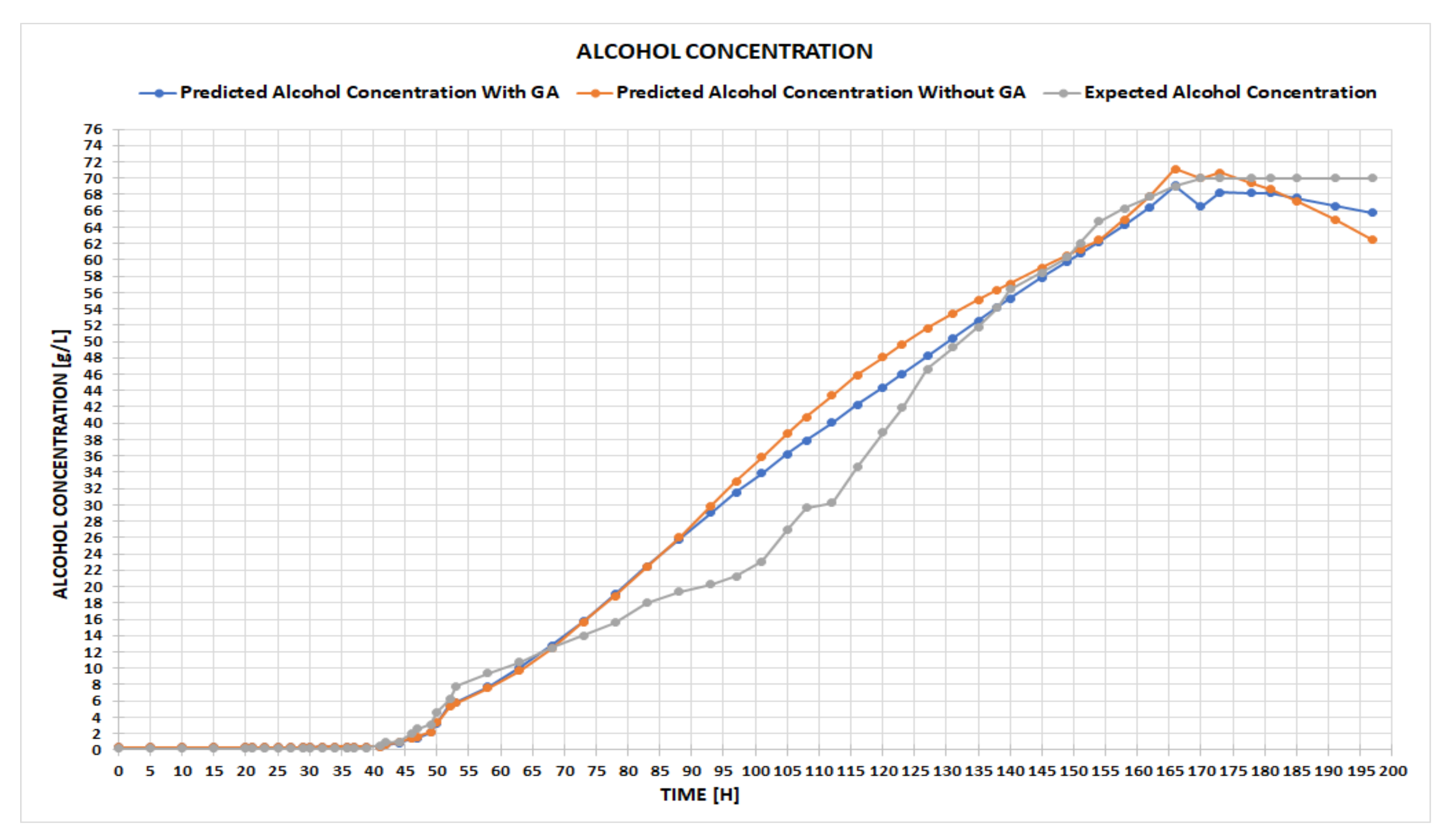
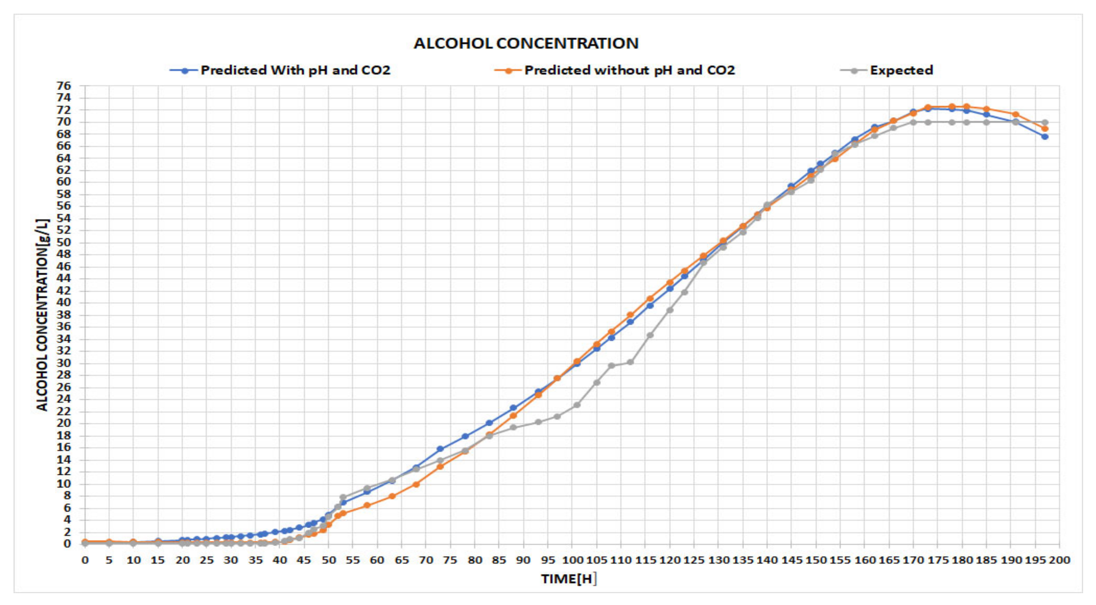
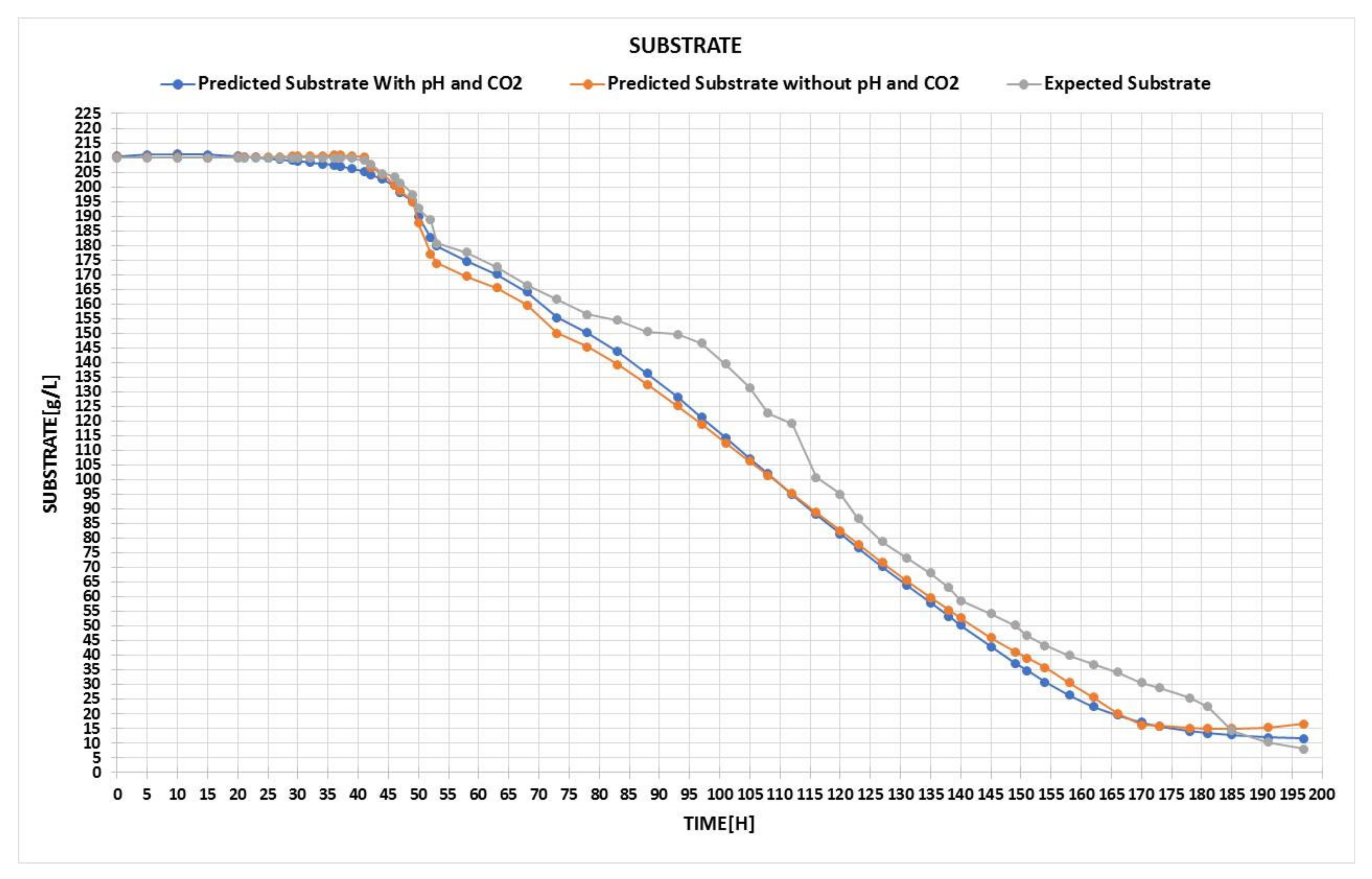
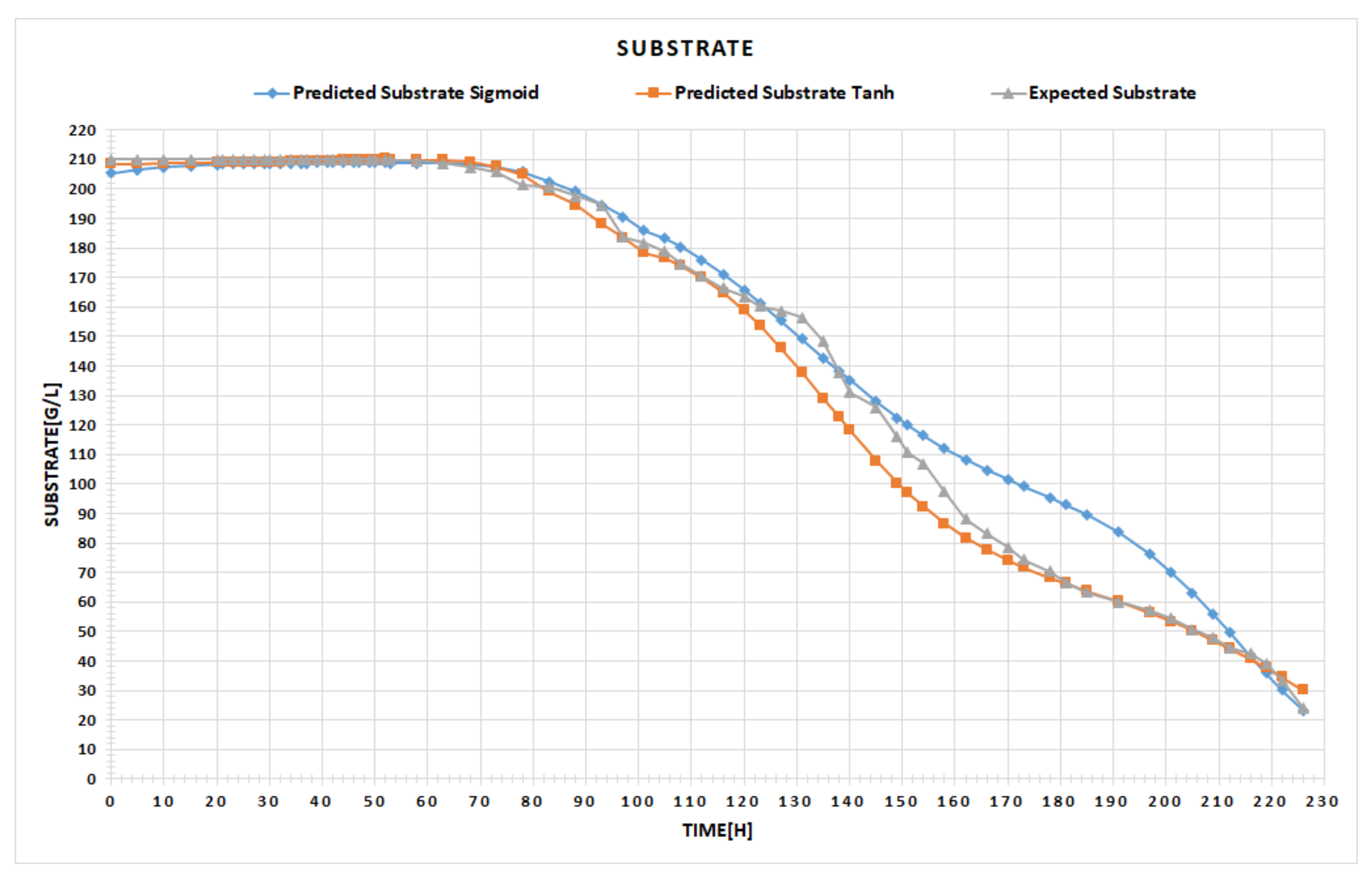
For this study, the alcoholic fermentation experimental processes have been conducted in a bioreactor (EVO, 10 L, software NEPTUNE, Pierre Guerin, France) in the research laboratory and have been divided into four distinct control situations. These concern the initial concentration of the substrate (210 and 180 g/L), the initial concentration of the biomass (0.1 and 0.2 g/L), the temperature values (20, 22, 24, and 26 °C), and the fermentation medium characteristics: mash malted, mash malt enriched with B1 vitamin (thiamine), white grape juice (Sauvignon Blanc must) and white grape must (Sauvignon Blanc must) enriched with a B1 vitamin (thiamine). For the experiments, the wine yeasts Saccharomyces oviformis and Saccharomyces ellipsoideus were used, these being seeded on a culture medium [15]. During the process’s evolution, the cell concentration has been calculated on the basis of three different measurements: optical density, dry substance, and the total number of cells. The ethanol concentration has been determined using HPLC-MS (Agilent, USA, Agilrom, Bucharest, Romania) equipment and the substrate concentration has been determined with a spectrophotometric technique.

The bioreactor has been equipped with sensors and analyzers to monitor pH, temperature, level and stirred speed control, dissolved O₂, and the released CO₂ and O₂. From the obtained experimental data, based on the domain knowledge of the authors, 30 “representative” sets were used, considering the following contexts obtained from a combination of variables: 210 and 180 g/L as the initial concentration of the substrate, 0.1 g/L as the initial concentration of the biomass, the four mediums, and the four temperatures.

To be able to predict the process parameters, we followed the steps presented in Figure 1 algorithmically. The proposed solution was to create a tool based on a neural network that could be trained by using data from the bioreactor, in such a way that it could predict the output variables as accurately as possible.

Although neural networks have previously been successfully applied in control processes [16], from our experience, we can say that there is no single solution (in terms of NN configuration) to suit all problems. For this reason, we believe that cross-fertilizing ideas belonging to evolutionary computing (such as automatic design space exploration, based on genetic algorithms) with artificial intelligence (neural networks) can lead to better results. Thus, we tried to improve and enrich the current solution by replacing the manual design -space exploration for the architecture of the NN with a basic, automatic design space exploration based on a genetic algorithm. The idea started from the fact that several parameters of the NN are chosen randomly at the beginning of the process, such as the weights, the number of hidden layers, the number of neurons on a hidden layer, and the learning rate. More precisely, the aim is to replace the initial random weights of the NN with some that are generated by the genetic algorithm, run for between 30 and 50 generations, in order to increase prediction accuracy. To achieve this goal, an NN has been developed in Visual Studio C# and trained using the experimental data for an alcoholic fermentation process from white winemaking; then, based on this NN, we have been predicted the desired variables of the process.

The application development stages consisted of:

• The back-end component implements the functionality of the application—the configuration of the neural network and its prediction. After compiling this application, a dynamic library file is obtained that will be included later in the graphical interface.
• The front-end component contains all the design and presentation features of the application. It was created with the help of dynamic ASP.NET pages, which were developed using the structure and elements typical of the HTML 5.0 language and including controls such as buttons, tags, and text boxes, specific to the ASP.NET standard. To stylize and place these elements on the page, we used CSS and JavaScript. Through this implementation mode, the application is available remotely, facilitating its operation without the need to be near the bioreactor.

The neural network was trained using experimental data obtained from the bioreactor wherein the fermentation occurred. The data were collected either by samples acquisition and analysis or from the transductors. Different datasets were used in the training and testing steps, which contain some or all of the following process variables:

• Temperature;
• Biomass concentration;
• Time;
• Initial substrate concentration (glucose);
• Substrate concentration at time t;
• CO₂ concentration;
• Evolved oxygen concentration;
• pH.

Based on the input, two different configurations were outlined: the first one used only 4 parameters, such as temperature, biomass, time, and initial substrate, while the second one used 2 additional inputs of CO₂ concentration and pH.

2.1. User Guide and System Requirements

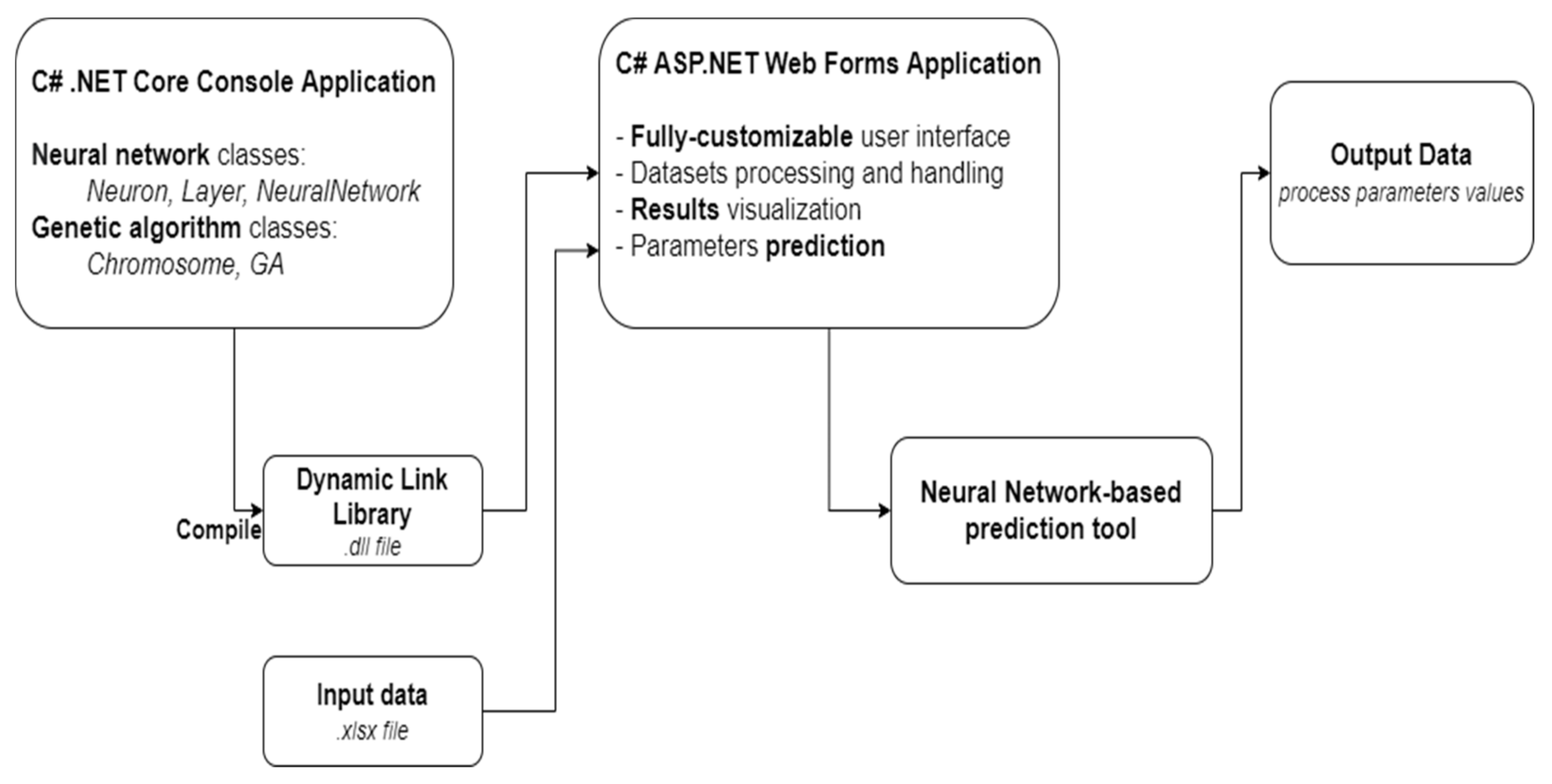
The software application was developed in Visual Studio IDE with C# in 2 different phases: the so-called “back-end” implementation, wherein the architecture of the overall project was designed, and the “front-end” implementation, wherein a user-friendly interface (UI) was created based on an ASP.NET Web Forms Application in order to remotely monitor the fermentation process. This way, we could ensure that the software solution that is proposed is easily portable and platform-independent; thus, migrating it to a Linux/Android/iOS machine would require only a new UI, instead of having to create everything from scratch.

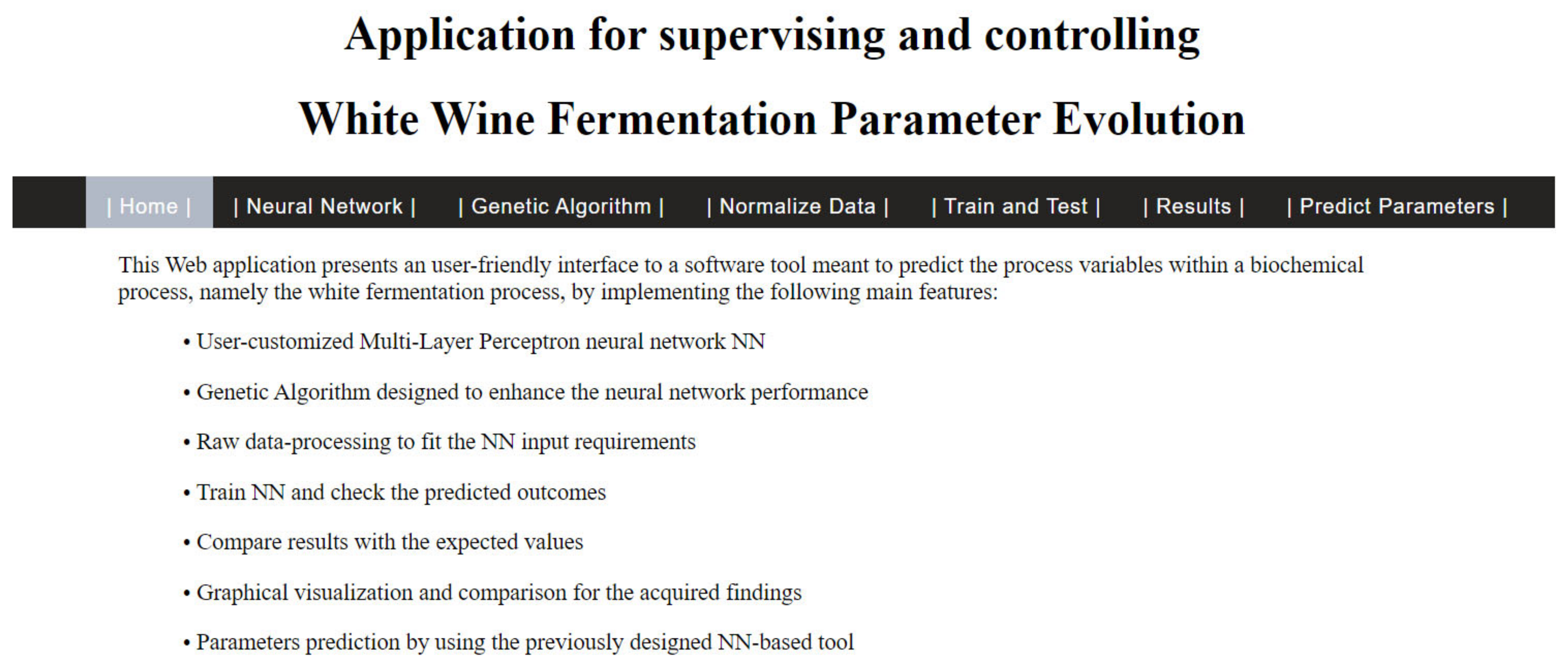
The graphical interface, or the front end, was developed as a website, with one menu bar and several dedicated web pages so that it could facilitate remote access by an expert. The menu bar allows the end-user to easily navigate throughout the different stages of the prediction process, as can be seen in Figure 2.

Through this software application, the user can accomplish the following tasks:

• Choose an Excel (*.xlsx) file in which the training data of the network are structured.
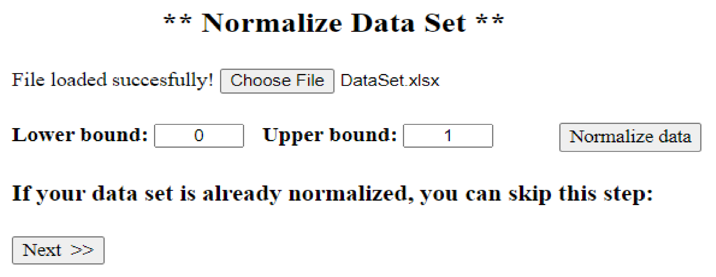
• Choose an Excel (*.xlsx) file for generating a normalized data set.
• Choose the type of network to predict the variables.
• Set up the iteration number that the network will execute in the training process.
• Set up the neuron number for the hidden layer of the network.
• Set up the number of hidden layers of the network.
• Comparatively visualize the graphics of the desired output of the network and the real output.
• Predict the desired variable functions of several variables, defined as the input network.

From a hardware point of view, to run properly, the application needs systems with quad-core processors, 8 GB RAM, and a minimum of 850 MB up to 20 GB of HDD available space, depending on the Visual Studio features installed. We created an archive using the sources of the applications, which can be accessed at the following web address (http://webspace.ulbsibiu.ro/adrian.florea/html/simulatoare/WineFermentationPrediction.zip (accessed on 20 February 2022)) and downloaded to local computers by any interested parties. We recommend using Windows 10 or a later version. Further details about the software’s use are provided by the README.txt file in the archive. This software application was developed using the full Visual Studio license provided for academic use, free of charge, by the Lucian Blaga University of Sibiu, with the full support of the Hasso Plattner Foundation in Germany. For this reason, those who use our source must do so only for educational purposes. Besides it being free and easy to use, our tool provides the following advantages: flexibility, extensibility, interactivity, and performance.

2.2. Architecture and Design

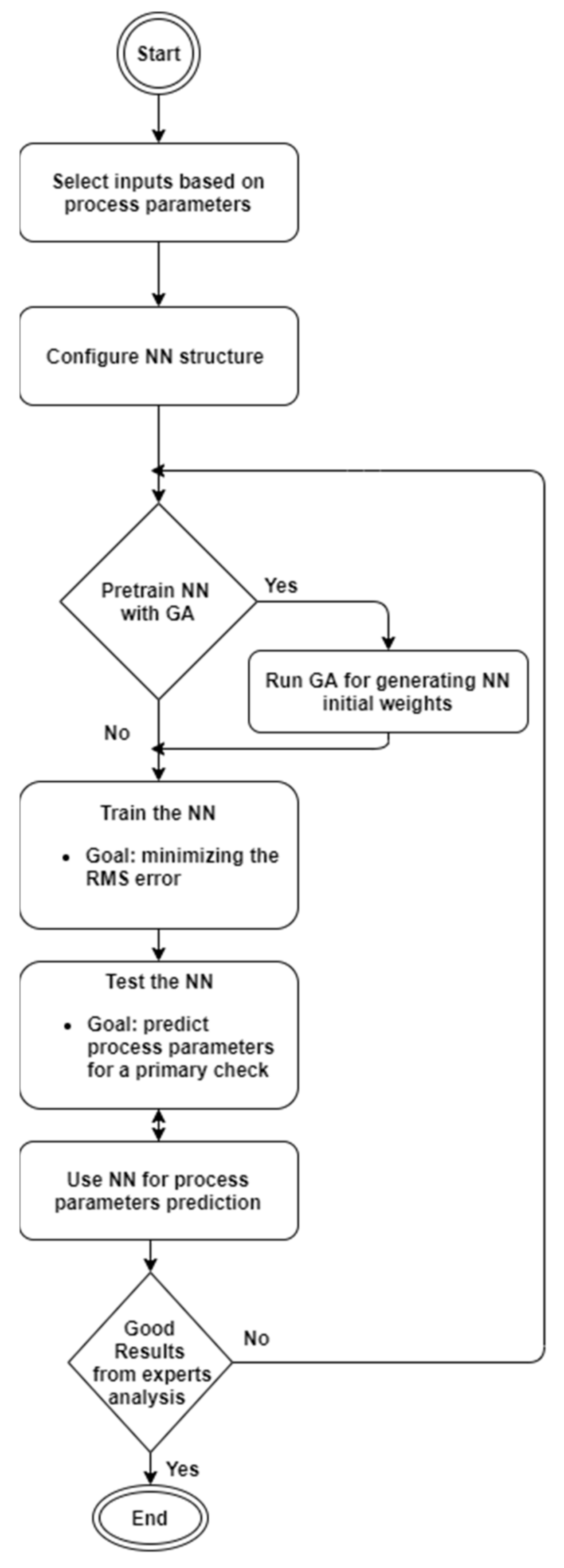
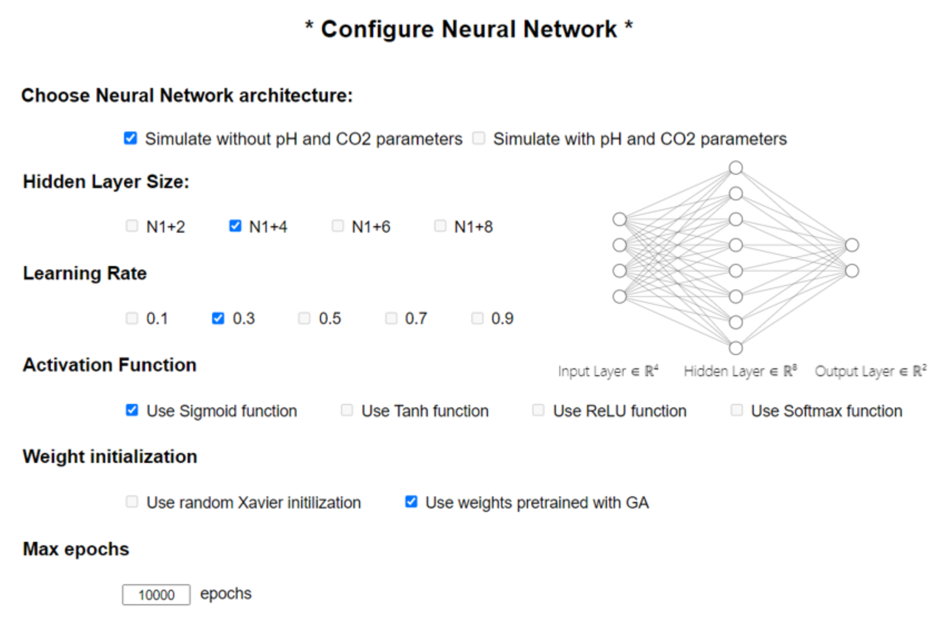
The menu bar displays all the steps required for the prediction process in a logical and chronological order, as shown in the diagram in Figure 1. The first step was to configure the neural network that fits the input dataset. We could perform this intuitively and easily from the graphical interface by using checkboxes and text boxes, as highlighted in Figure A1 in Appendix A. The user interface (UI) allows the user to select the type of data they want to use for the simulation from between the two possible choices previously outlined in Section 2. Their selection would influence the entire network architecture by changing the number of neurons on the input layer, denoted henceforth as N1. The application simulates a feed-forward multi-layer perceptron (MLP) network with a backpropagation (BP) algorithm. The backpropagation learning model is a learning algorithm used in feed-forward networks. BP comprises two steps: the first step (forward) is where information is passed from input to output, followed by a step from output to input. The forward step propagates the input vector to the first level of the network; the outputs of this level produce a new vector that will be the input for the next level until it reaches the last level, where the outputs are the network outputs. The second step backward (backward) is similar to the forward step, except that errors are propagated backward through the network to cause the weights to adjust. Based on gradient descent for weight adjustment, the BP algorithm uses the chain rule to compute the gradient of the error for each unit with respect to its weights. There are several other parameters that must be customized, such as: the number of neurons in the hidden layer, the learning rate, which in the literature is usually given the notation β, the activation function, the weights initialization, and the maximum number of epochs for which the network has to be trained.

For the activation functions, four of the most well-known functions in feed-forward neural networks were taken into consideration. Each one has its own advantages and disadvantages; it is up to the user to choose the function that best suits the input data. Although the sigmoid (Equation (1)) and hyperbolic tangent (Equation (2)) are two of the most widely used functions, they both face the problem of vanishing gradients. As an alternative, there is the ReLU function (Equation (3)), which stands for the rectified linear unit; this is meant to activate only those neurons that have a significant output (higher than 0). Another option to the well-known sigmoid function would be SoftMax (Equation (4)).

$$f\left(x\right)=\frac{1}{1+e^{-x}}$$

(1)

$$f\left(x\right)=\frac{e^x-e^{-x}}{e^x+e^{-x}}$$

(2)

$$f\left(x\right)=\max \left(0,x\right)$$

(3)

$$softmax\left(z_i\right)=\frac{\exp \left(z_i\right)}{{{\displaystyle \sum }}_j{z}_j}$$

(4)

For the weight initialization step, there are two different approaches we considered that best suited our dataset. The first approach is a pseudo-random initialization that generates sub-unitary values, called the Xavier initialization [17]. Instead of generating completely random weights in the (0, 1) domain, this initialization chooses values from a random uniform distribution, bounded by the following interval:

$$\left[-\frac{\sqrt{6}}{\sqrt{n_i+n_{i+1}} },+\frac{\sqrt{6}}{\sqrt{n_i+n_{i+1}}}\right]$$

(5)

where $n_i$ is the number of incomings in terms of network connections and $n_{i+1}$ is the number of outgoing network connections from that layer. Assuming that the configuration selected for the neural network in Figure A1 represents a 3-layer MLP neural network (Input–Hidden–Output), for the hidden layer, the value of $n_i$ would be the number of the neurons on the input layer and $n_{i+1}$ the number of neurons on the output layer.

The other approach is the one that brings innovation to our application, i.e., finding the initial weighting configuration that yields the best results by using a heuristic algorithm, such as a genetic algorithm. The original premise was that finding an optimal layout for our network can be narrowed down to a searching problem within an infinite space of solutions. It has previously been established that an exhaustive search would be time-consuming and pointless, which is what led us to use heuristic methods, among which the best-known one is the genetic algorithm.

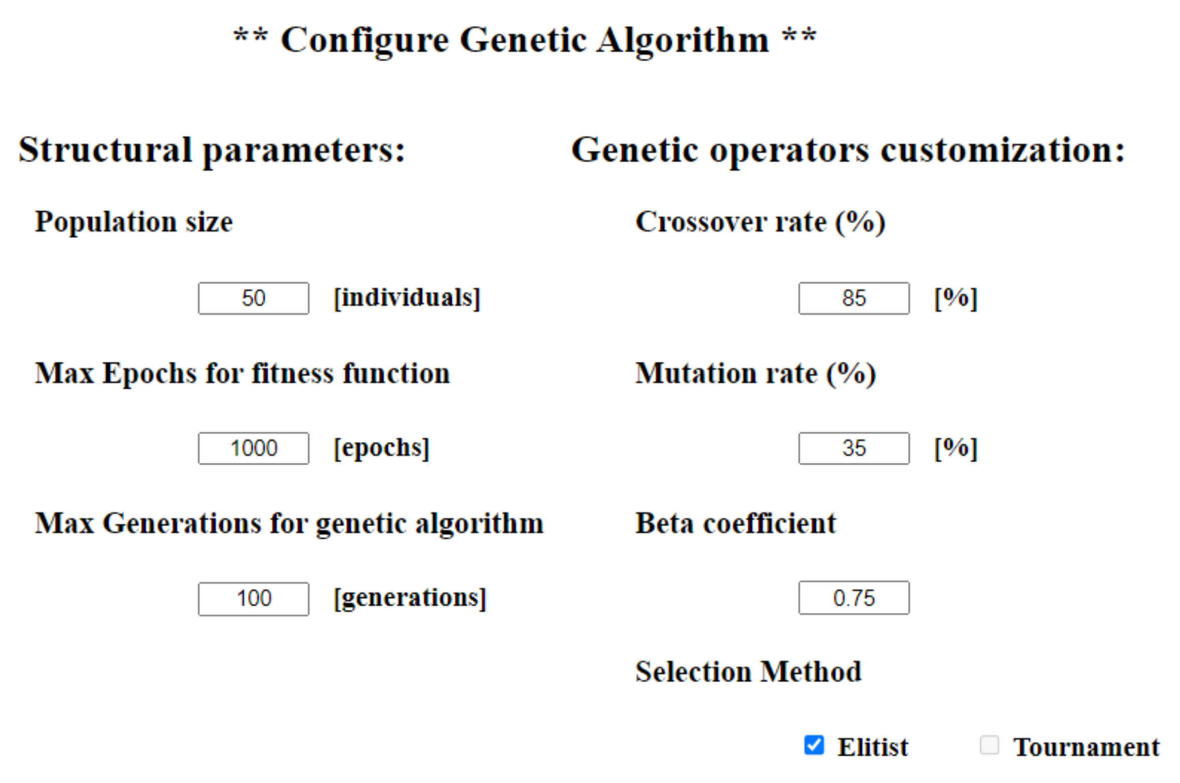
For this to be possible, we had to exclude the easy and intuitive approach of using the neural network libraries proposed by MATLAB (also used by us in a previous work [16]) and create our own user-customizable solution, with the help of C# and the ASP.NET framework. Akin to implementation for the neural network design, the expert user is given the opportunity to fully customize the genetic algorithm operators using the controls offered by the ASP web pages, such as text boxes and checkboxes (Figure A2).

The process starts with a population of randomly generated individuals. In our approach, each individual represents a different neural network, with its own generated weights. To narrow it down to a simple approach, the individual can be represented as a linear matrix of weights, as follows:

Here, each weight is generated with the above-mentioned Xavier initialization. In Figure 3, we are using the NN selected in Figure A1 (from Appendix A), wherein we set 4 neurons on the input layer, 1 single hidden layer with 8 neurons, and 2 neurons on the output layer. The fitness function used to evaluate each individual is the backpropagation algorithm itself, while the fitness score is the output of this algorithm, i.e., the network error that resulted after training the network for the specific number of epochs selected by the user. The number of individuals selected for the initial population and the maximum number of generations is again selected by the user; this must be a trade-off between having an optimal solution and a proper execution time.

Each individual has a finite number of genes, which in our case are represented by the linear matrix of weights, where one weight corresponds to one gene. Each string of genes, also called the chromosome, is a possible solution to the search problem. In order to find the optimal configuration, we applied the three genetic operators to the initial population. As previously mentioned, the application is fully customizable, as this is its main purpose and, although there are many proposals for this type of crossover, mutation, or selection, we implemented only the ones that best suited our dataset and that provided acceptable results. Hence, as a parent selection method, either the elitist method, which chooses the two individuals with the best fitness score, or the tournament method, which selects the two best-evaluated individuals among several n of randomly selected individuals, can be chosen. The latter choice follows the principle that it is not always the first, best, 2 parents that generate the best offspring, giving the chance for weaker evaluated individuals to participate in the crossover process.

As for the crossover process, there are several well-known methods, such as the k-point crossover, uniform crossover, or order-based crossover. For our solution, we opted for a probability-based uniform crossover.

Here, W¹_i,j and W²_i,j are the genes of the parents, arising from the selection process. More precisely, for each gene of the selected chromosome, a random probability P is generated; if the generated P is less than the crossover probability, denoted as P_crossover in Figure 4, or the crossover rate in Figure A2 (in Appendix A), the value of this gene is exchanged with the value of the corresponding gene of the second selected chromosome. It is advisable that in all cases, no matter the data set used, the crossover rate needs to be high enough to ensure that the future generation is somehow distinct and can bring improvements compared with the previous generation.

After crossover, the mutation operator will be used in order to bring diversity to the population with its best-known types: bit-string mutation, flip bit, boundary, uniform, or Gaussian. Conversely to the high rate of the crossover, the mutation probability must be low enough not to generate completely new random offspring while still bringing diversity to the population. We have chosen a probability-based uniform mutation (Figure 5), but it is dynamically handled this time; we started with a user-defined mutation probability and adjusted it with each generation, as follows:

$$P_{mutation\_new}=P_{mutation\_old}\times e^{\left(1-generatio{n}_{no}\right)\times Beta}$$

(6)

where Beta is a sub-unitary coefficient selected by the expert user in the configuration box (Figure A2).

After applying these operators, we have a group of individuals comprising the initial population and the newly generated offspring. The latter are evaluated using the same fitness function and, based on the fitness score, we replace the worst-evaluated individuals with the two derived descendants if they perform better than these individuals. Consequently, the survival of the individuals in the new generation is based on an elitist approach.

These operators are applied repeatedly to the group of individuals until the population converges, meaning that it does not produce significantly better-scored offspring, or until the maximum number of generations has been reached. In the end, the outcome is an individual representing the best or at least the optimal configuration of initial weights for our neural network.

2.3. Data-Processing

At the beginning of Section 2, the structure of the input data sets is detailed: we are using real values, determined by laboratory measurements of temperature, substrate, biomass, time, CO₂ concentration, or pH. There is a clear discrepancy between the high values for these parameters and the values returned by our activation functions—thus, the need for normalization.

Based on the lower and upper bounds selected by the user, each value is recomputed using the following formula:

$$x^{\prime }=mi{n}_{new}+\frac{\left(x-mi{n}_{old}\right) \times \left(ma{x}_{new}-mi{n}_{new}\right)}{ma{x}_{old}-mi{n}_{old}}$$

(7)

where $mi{n}_{new}$ and $ma{x}_{new}$ represent the lower values, respectively, from the upper bound selected in the textboxes in Figure A3 in Appendix A, and $mi{n}_{old}$ and $ma{x}_{old}$ represent the minimum and the maximum values, respectively, of the raw parameters from the input data. By $x$ we denote the current value that we want to process, and by $x$’, the resulted value after normalization. Each value from the original data set from the ith row and jth column will be saved in the new spreadsheet in the corresponding cell.

If the user already has the processed data set that fits the network’s inputs, this step can be skipped, either by going directly to the Train and Test section with the aid of the navigation bar or by pressing the “Next” button in the interface.

2.4. Prediction Tool

The neural network architecture selection is now complete, ready for training, and, finally, for testing. In order to do that, the spreadsheet format datasets will be used for both training and testing, as follows: the user must select the sets used for training by checking the corresponding boxes in the application. In our experiments, the training/testing ratio is 75/25 because we used 3 data sets for training and one for testing (see the configuration from Figure A4 in Appendix A). However, if we vary the number of sets on which we perform, the practice test, we also change the training/testing ratio of 75/25. Our application is flexible and allows having many configurations (for example, 50/50, or even 25/75. Considering n ($n\ge 2)$ benchmarks (data sets) and that we use k benchmarks ($n>\mathrm{k}\ge 1)$ for training, we must have at least one set for training and the rest for testing, with at least one set for testing, although it is recommended for better results that more than 50% of the data is reserved for training. The total number of configurations that can be simulated is:

$$C_n^k·\left(C_{n-k}^1+C_{n-k}^2+\dots +C_{n-k}^{n-k}\right)=C_n^k·\left(2^{n-k}-1\right)$$

(8)

For example, selecting only one benchmark for training the total number of configurations that can be simulated is $C_n^1·\left(C_{n-1}^1+C_{n-1}^2+\dots +C_{n-1}^{n-1}\right)=n·\left(2^{n-1}-1\right)$, because we may select anyone from all n benchmarks for training, and for testing, one from all n − 1 remaining data sets or select two from all n − 1 for testing, etc. Taking all these into consideration, we consider that the training/testing sets are representative of all combinations of the experimental conditions.

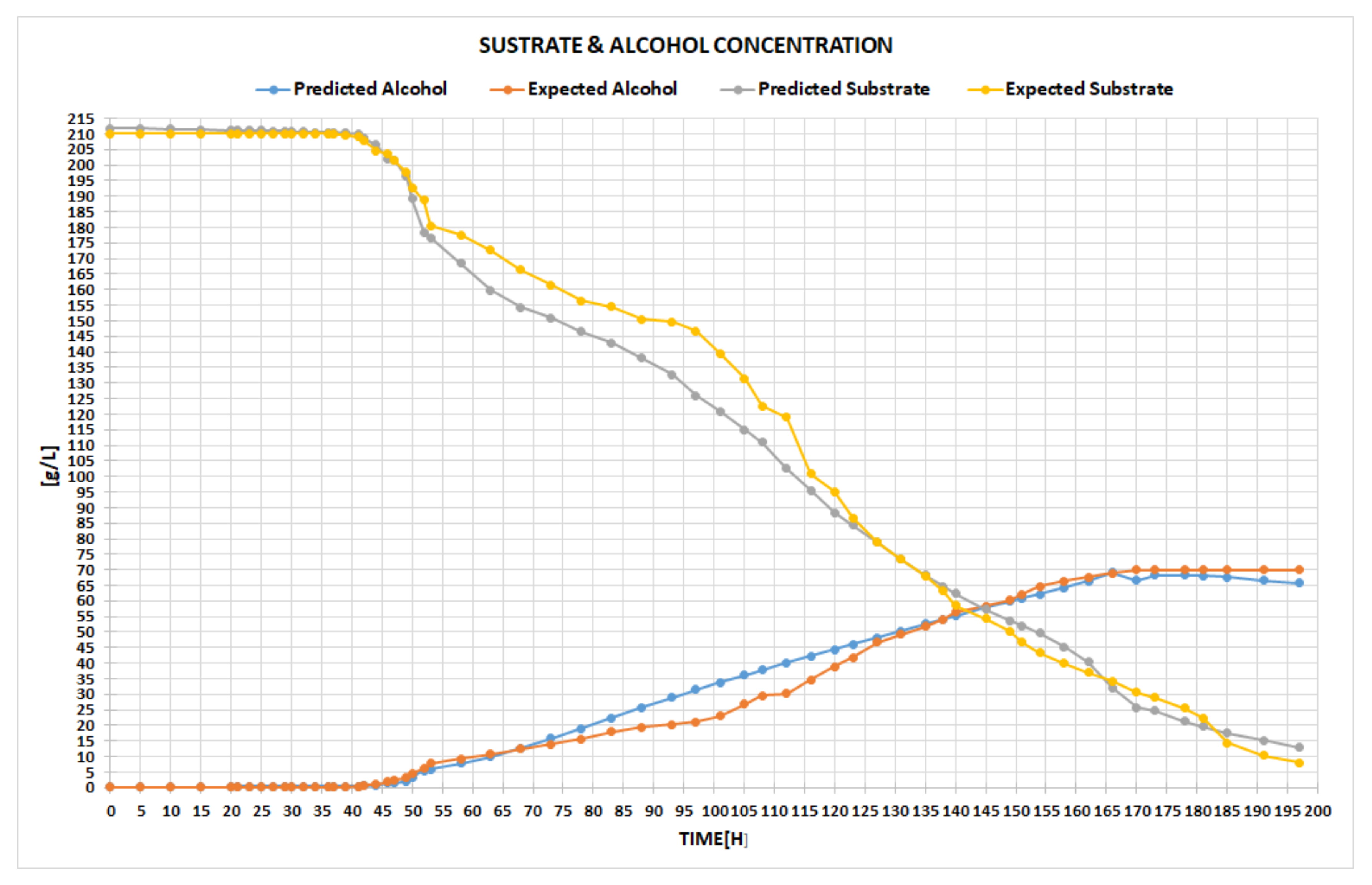
The expected output can be checked in the results section (Figure 6), designed to accelerate the interpretation process by laying out both numerical and graphical results. The training and testing errors give important values for a first evaluation; there are situations where the training error is very low but the testing error is still high, so that we can safely conclude immediately that we are dealing with an overfitting problem (the model learns the detail and noise in the training data, to the extent that it negatively impacts the performance of the model with new data). Still, for a deeper evaluation, the graphics containing the results from the test are more meaningful.

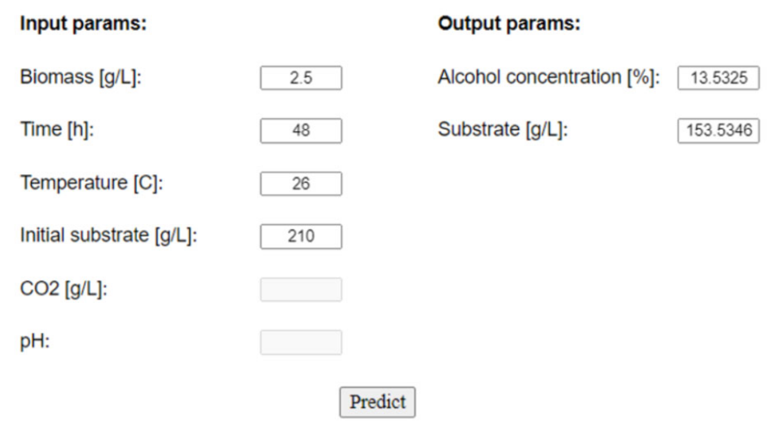
The left-hand chart in Figure 6 highlights the expected ascending curve of alcohol generation, versus the one predicted by our network in the testing phase. The right-hand chart displays the expected quantity of the consumed substrate in time, compared to the one attained within the testing period. The user can switch between different chart types, for instance, by point, line, bar, column, or area, the main idea being to select the particular type of chart that better emphasizes the visual differences between the data. With all these facts being given, the expert can now conclude whether the results are satisfactory or not. If yes, the final step is to use the obtained tool for the prediction process of the fermentation parameters, as the example in Figure 7 indicates.

In the left-hand input section, the user is required to fill in the boxes with the values of the process parameters, meaning the quantity of biomass and initial substrate at a certain time and temperature. Temperature is very important because even the slightest fluctuation can alter the oxidation of the wine and, therefore, significantly affect the quality. Additionally, information about CO₂ and pH can be used if the neural network architecture is designed and trained with this information from the beginning. This example outlines the usage of the tool for the neural network built in Figure A1, with only 4 input parameters; thus, the last two boxes are disabled.

When pressing the “Predict” button in the output section, the numerical values for the output parameters can be read and further interpreted by the wine technology expert. Thus, the NN is able to determine the fermentation stage (providing real-time information regarding the fermentation process without reading the sensors) or predict wine quality based on the process variables. This can directly affect the productivity of the winery by saving time and money.

2.5. Core Application

As the overview in Section 2.1 highlights, the application was developed in two stages, i.e., the front-end part, which was described in depth in the previous sections, and the back-end part, which contains the core of the application with all its classes, members, and methods (see Figure 8). The latter component is the one that is meant to be portable; thus, it was developed as a separate entity from the user interface (UI) by using the .NET core framework. In order to finally integrate it into the UI, the whole code project was compiled into a dynamic link library, in other words, a .dll extension file, which was later included in the front-end ASP.NET Web Forms application project.

3. Results and Discussion

The final results presented in this chapter reflect the best performances that the tool could achieve, using the architecture and the design that are presented above. Besides presenting simulation results that are very close to the real measurements, the purpose of this tool is not only to demonstrate that we were able to design a perfectly working AI tool but also to show the advantages that an AI hybrid tool comprising an NN and a GA could bring compared to a basic NN tool.

3.1. Datasets

The simulations were performed repeatedly with different configurations for the neural network on 2 main types of data sets, as described in

Table 1. Data sets used for training and testing the NN (in and out parameters).

	DATASET 1	DATASET 2	SIGNIFICANCE
INPUT	T	T	Temperature (°C)
	t	t	time (h)
	S0	S0	Initial substrate concentration (g/L)
	X	X	Biomass concentration (g/L)
		pH	pH
		CO2	CO2 concentration released (percentage volume)
OUTPUT	P	P	Alcohol concentration (g/L)
	S	S	Substrate concentration (g/L)

.

The input data were previously obtained from experimental measurements and stored in spreadsheet files, wherein each column would contain the values of the input parameters at a specific moment in time t. Data were stored separately, depending on the value of the temperature at which the fermentation took place.

3.2. Simulation Prerequisites

The first simulations were performed as a test, in order to find the range wherein the parameters could vary, thus determining the configurations that could possibly lead to the best or the optimum solution. Although the final architecture of the prediction tool is subject to the discretion of the user, we had to narrow down an infinite number of possible parameters into only a few. The final solution was described in Section 2, along with all the possibilities and variations.

Furthermore, different simulations were performed with several NN configurations, with or without the GA. Some of the best results provided by our prediction tool, along with their interpretations, are provided in Section 3.3.

3.3. Graphical Results and Interpretations

3.3.1. Predicted vs. Expected Results

Different types of graphical data were built, in order to best evaluate our developed tool. In Figure 9, the output for the alcohol concentration and the one for the substrate are merged in the same graph.

For this simulation, the biomass (X), the initial substrate (S₀), the temperature (T), and the time (t) were used as the input parameters to the following NN:

• Input layer N1 = 4 neurons, one for each input parameter;
• Hidden layer N2 = N1 + 6 neurons, where N1 is the number of neurons on the input layer;
• Output layer N3 = 2, one for the alcohol concentration (P) and one for the substrate (S)
• Maximum number of epochs = 200,000;
• Training sets: sets with T = 26, 24 and 20 °C;
• Testing set: T = 22 °C;
• Weight initialization: weights that are pre-trained with the GA:
  • Population size = 50 individuals;
  • Crossover probability P_crossover = 0.9;
  • Mutation probability P_mutation = 0.5;
  • Mutation beta coefficient = 0.3;
  • Selection method: elitist;
  • Maximum number of generations = 50;
• Activation function: the sigmoid function;
• Learning rate = 0.7.

A few points can be extrapolated from this graphical representation, the first one being the fact that the ascending slope of the expected alcohol concentration (the orange line) and the descending slope of the substrate concentration (the yellow line) are not smooth at all, this being the result of the fact that the input data were raw and were not processed in any way. Still, both the expected and the predicted results are according to the real process: the alcohol concentration slope is ascending, a result that we expect from the fermentation process, based on the consumption of the substrate (the yeast produces alcohol with the consumption of the sugar). The higher the concentration of alcohol, the lower the substrate, until, at some point in time, the lines cross each other. Very importantly, the accuracy is also limited by the size of the data set, more precisely by the number of pairs in the training data presented to the neural network. With a maximum of 200 input-output pairs, the smallest training error obtained was about 3 × 10⁻³ for the sigmoid activation function, a hidden layer with 10 neurons, and pre-training the weights with the genetic algorithm.

On the same figure, we can distinguish the three fermentation phases:

• Lag phase: the first phase of the process, shown in Figure 9, wherein both the alcohol concentration of alcohol and the substrate stagnate;
• Exponential phase: starting with t = 50 h, where significant growth in the alcohol content can be noted, based on the substrate consumption;
• Stationary phase: starting from t = 150 h, the output parameters do not undergo major changes.

Thus, we can conclude that our results comply with the real-world process. Although there are small differences between the expected and the predicted results, the graphic of the results generated by the neural network tool cannot reach the spikes of the real experimental data.

3.3.2. Random Initialization vs. Genetic Algorithm Initialization

The initialization of the weights has a major influence on the performance of the neural network; therefore, we opted for the implementation of a heuristic optimization method like the genetic algorithm, in order to obtain a solution close to the optimal configuration. Comparisons between the best results that were achieved with a pseudo-random Xavier initialization and the ones that were achieved with GA initialization can be checked in Figure 10 for the alcohol concentration and in Figure 11 for the substrate quantity.

We achieved better results with the neural network pre-trained with the genetic algorithm, with a testing error of 0.03 compared to 0.045 in the case of the pseudo-random Xavier initialization. The previously mentioned error is the mean root square error used for an evaluation of the performance of the backpropagation algorithm. Although the integration of a genetic algorithm is time-consuming, the possibility of parallelization exists, the evaluation of each chromosome being independent one from the other. Thus, for higher performance and a decreased simulation time, each performance evaluation, meaning each backpropagation algorithm, could run on a different software thread on multicore processors in LAN or HPC systems. With this approach, the evaluation time drops significantly; thus, this approach is achievable. To reduce the simulation time, there are a number of free resources available from major software developers, such as Google and Microsoft. Among these resources, we find virtual machines, storage, databases, tools for developers, etc. These resources are not permanently free; it is only for a limited number of months. For this work, we used Windows Virtual Machines; these resources were provided by Microsoft Azure for students of the Lucian Blaga University of Sibiu (ULBS), free for 12 months, based on authentication with a valid Gmail (ULBS) account.

3.3.3. Data Sets Comparison

There was an increase in the prediction accuracy once the additional information about the pH and the released carbon dioxide was incorporated, leading to the conclusion that a larger amount of data positively influences the performance of the neural network (Figure 12 and Figure 13).

Following analysis of the simulations in Figure 14, we concluded that a large number of epochs does not guarantee a higher prediction accuracy; on the contrary, for very high values, the performance decreases because the network error has exceeded the minimum possible value overall. Our study shows us that in some cases, the hyperbolic tangent function is more efficient than that of the sigmoid in terms of predictive accuracy. For both activation functions, the results given by the neural network follow the graph of the expected function, the alcohol concentration increases over time, and the amount of substrate decreases. In conclusion, network training with a very large number of epochs is useless in terms of performance, backpropagation being a slow learning algorithm, based on the principle of error correction, which initially changes significantly; later, the difference becomes smaller. Thus, the gain is too small compared to the computing power consumption required for a large number of epochs.

In terms of activation function, the sigmoid and hyperbolic tangent (tanh) functions performed similarly but demonstrated different learning rates. The sigmoid function performs better for higher learning rates, while the hyperbolic tangent function performs better for lower learning rates (as Figure 15 reveals). For each pair of output values—expected value, for each time moment, t, we calculated the difference between the two values. In the case of alcohol concentration, the largest difference was 11.02 g/L, at the time t = 212 h, for sigmoid function, and 12.76 g/L at time t = 219 h, for the tanh function. In the case of the substrate quantity, for tanh, the maximum error is 19.44, and for the sigmoid function, 26.36. In the case of the latter, the difference is significantly greater, and this can be seen in the graph of the function.

4. Conclusions and Further Work

This paper proves the possibility of integrating the field of artificial intelligence and machine learning into fermentation bioprocesses. This is a hybrid work combining two different fields, computer engineering and food engineering, showing the usefulness and necessity of digitalization in the development of processes in today’s industrial climate. The study consisted of the implementation of a software application that models the functionality of a fully configurable 3-layer feed-forward multilayer perceptron neural network, which based on previously obtained experimental data, can predict the evolution of the quantities characteristic of the alcoholic fermentation process of white wines. The main contribution of this work is that we show the superiority of an AI hybrid tool composed of a neural network and genetic algorithms, with the advantages it brings compared to a basic neural network, in predicting the process variables of wine fermentation.

After comprehensive simulations using experimental data obtained from previous fermentation processes, we concluded that the configuration that is closest to optimal, for which the prediction accuracy is high, is a neural network (NN) with an input layer having N (4 or 6) neurons, one hidden layer with N + 6 neurons, and 2 neurons on the output layer, running for 50,000 iterations and pre-trained with a genetic algorithm. With a larger number of neurons on the hidden layer, the training time increases, but this is not reflected in the NN performance and the difference in prediction accuracy is not significant. The optimal configuration of GA has a population of 50 individuals and runs for 20 generations, with a crossover probability of 0.9 and a probability of mutation of 0.5 that uniformly decreases depending on the number of generations, based on a beta coefficient of 0.3 and an elitist selection method. Although a larger number of individuals means the integration of more possible solutions in the search space, increasing this also means increasing the time and computing power consumed; in our case, this increase was not justified by the obtained results. Using pH and CO₂ as inputs of the NN, the prediction accuracy is higher, so we can conclude that a larger data set positively influences the performance of the artificial neural network.

The current work discusses one of a variety of research applications in the field of bioengineering, a field undergoing great development in which the need to find methods for the control and automatic monitoring of processes is growing. All these methods based on artificial intelligence and machine learning applications, such as neural networks, fuzzy logic, and support-vector machines, along with various heuristic optimization methods, such as genetic algorithms, ant colony model optimization, simulated annealing, etc., are essential if the hardware sensors cannot be used or if direct measurements cannot be made. For this reason, further research and development in this area are needed for both the food industry and other industries that require automatic process supervision. The importance of existing hardware methods is high, based on using them to obtain the experimental data needed to develop software solutions.

In further developments, we will consider the modification of the architecture of the neural network in terms of the number of hidden layers (using a deep neural network) and the activation function used, like SoftMax, ReLU, or Leaky ReLU. We intend to extend and model the software’s application so that it can be integrated into other fermentation processes for automatic management, as well as testing the alcoholic fermentation of red and rosé wines.