Transition to the Fluid Dynamic Limit: Mathematical Models and Simulation Results

Abstract

Numerical simulations of standard situations in the transition region from gas kinetics to fluid dynamics at small Mach numbers indicate a clear dependence of the simulation results on the underlying kinetic model (here: nonlinear and linearized Boltzmann collision operator vs. BGK relaxation model). We develop an improved mathematical framework (trace theory) to explain these differences. In particular we reveal certain deficiencies for the classical BKG system as well as for the standard Navier Stokes approach.

1. Introduction

Numerical simulations of flows in the transition from the gas kinetic (mesoscopic) to the fluid dynamic regime (macroscopic) represent a demanding task. On the mesoscopic side, the collision term operates on the six-dimensional phase space and is very complex. On the macroscopic side, including a collision term in the fluid dynamic equations makes the problem become numerically stiff and hard to resolve in time.

In this situation, simplifying models are en vogue. The most popular ones are systems of BGK type (Bhatnagar–Gross–Krook models, see [1]) which treat mesoscopic effects applying simple one- or more-parameter relaxation rules. Theoretical models try to find formulas from asymptotic analysis, taking into account the small mesoscopic perturbations as terms of an expansion with respect to some small parameter $ϵ$ (Hilbert, Chapman–Enskog expansion). From this, we find the Euler and the Navier Stokes equations as zeroth and first order approximations. Improved models, e.g., for a more detailed refinement of the pressure tensor are expected from higher order terms.

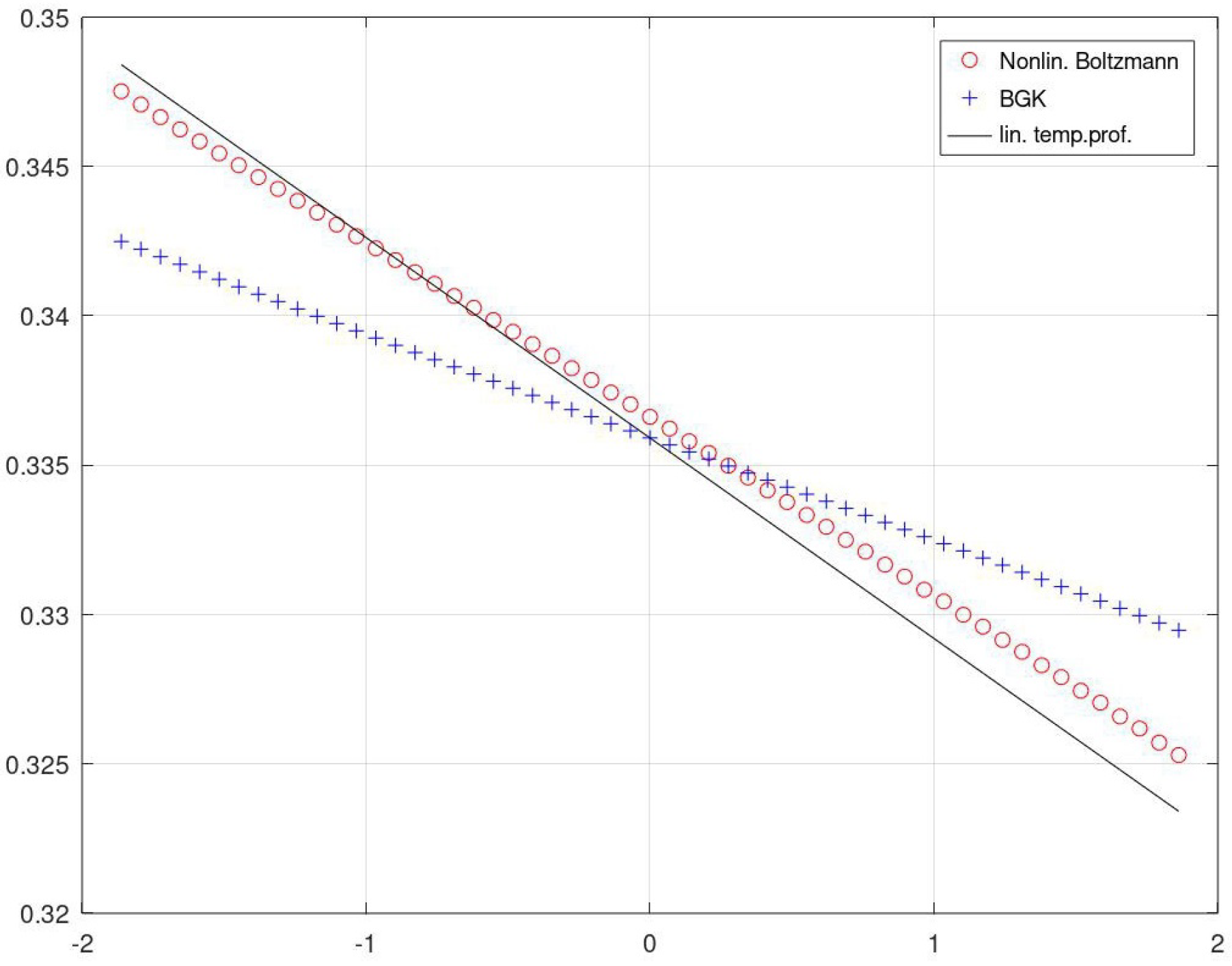
In the course of the present paper we demonstrate that all these models fail in certain practically relevant situations. E.g., the $ϵ$-expansion ansatz fails in some condensation-evaporation problems for a gas mixture (see Section 6.2), leading to some unphysical ghost effects. The BGK ansatz yields systematic errors even in simple heat layer problems (Section 6.1). In the following, we propose new ansatz (trace solutions) which works on the tangent space to the set of all Maxwellians (rather than the classical ansatz “solution = Maxwellian plus orthogonal perturbation”, supplemented with an exponential relaxation rule). As a motivation, we discuss the relaxation of a simple local perturbation problem (see Section 5.2). The crucial feature of the new approach is that (close to the fluid dynamic limit) the local macroscopic moments are not reflected by the local Maxwellian but by a specific moment perturbation.

The idea to construct intermediate states between arbitrary density functions and Maxwellians is not new. E.g., Shakhov [2] proposed such a system which is at present used for numerical simulations [3]. A comparable intention lies behind the idea of the extended BGK model with an additional relaxation parameter to match the correct Prandtl number, or related generalizations [4]. However, a better understanding of the transfer to fluid dynamics is not a question of parameter matching, and the above approaches do not yield a theoretical basis and a safe mathematical ground. Proposing a modified structure of kinetic solutions, the present paper claims to provide a new attempt to better understand the passage from the rarefied gas description to the macroscopic limit.

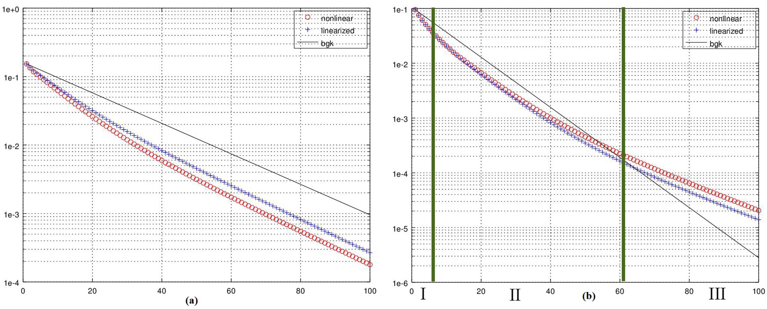
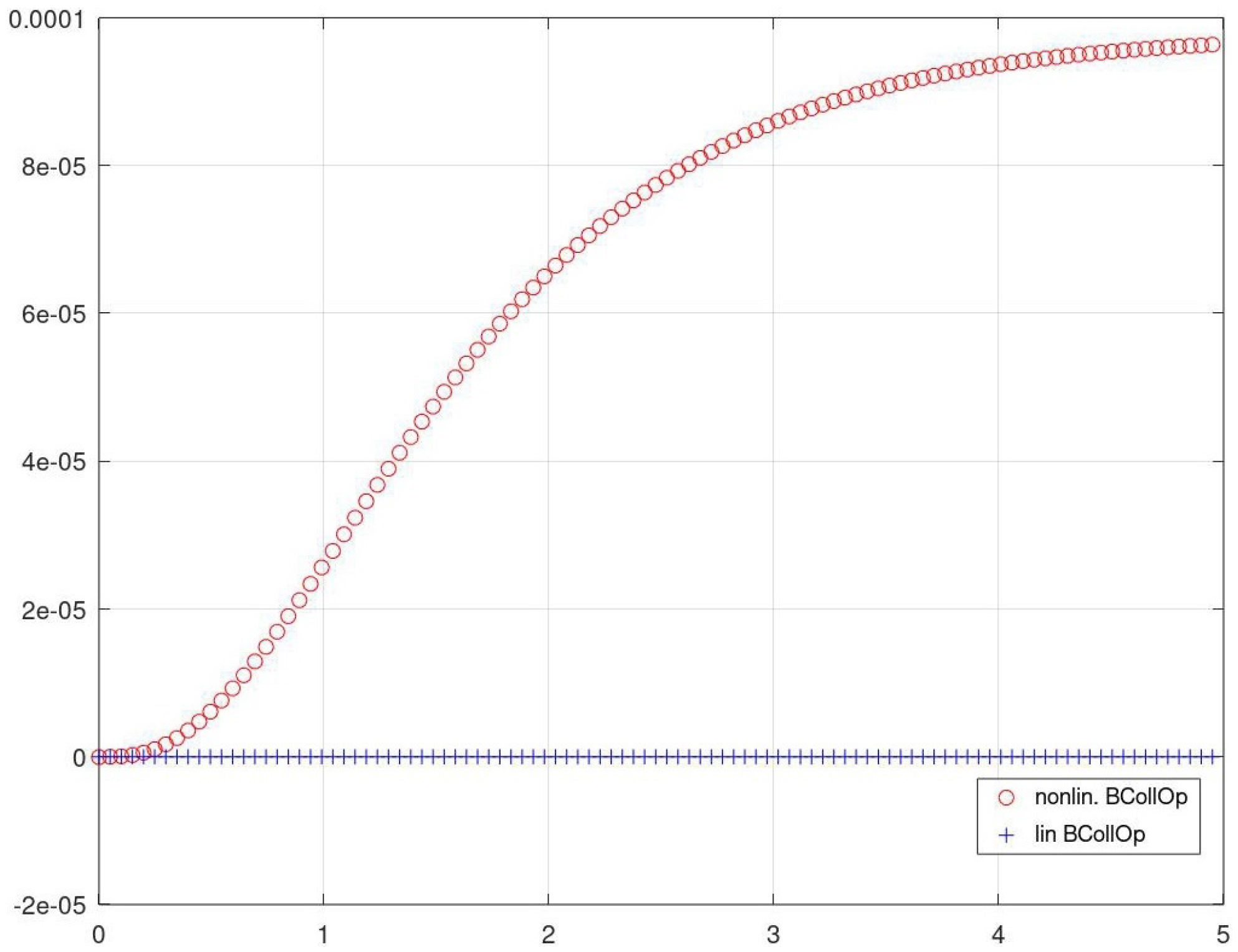
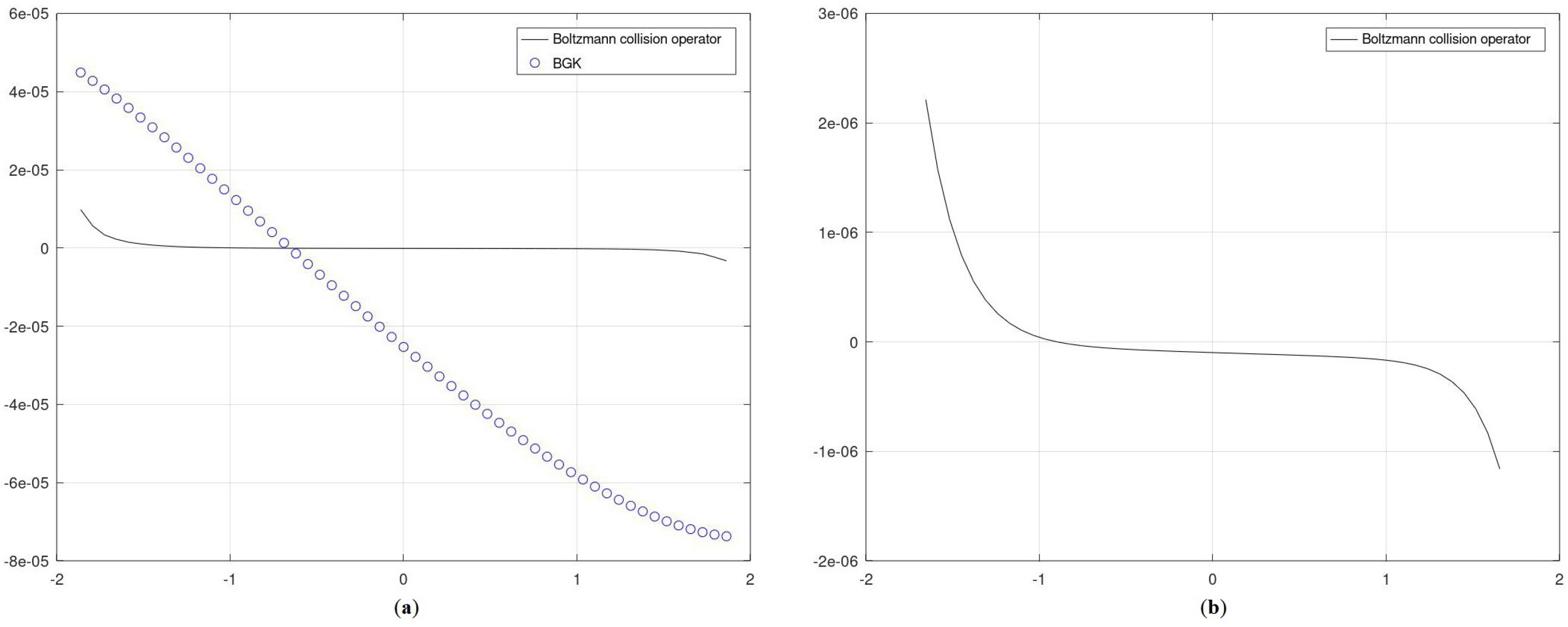
We derive closure relations which take the form of nonlinear first order (rather than second order) differential terms and thus are completely different from the parabolic second order terms of the Navier–Stokes system. The results allow one to interpret the differences in various kinetic models (here: nonlinear and linearized Boltzmann collision operators and the BGK relaxation operator) in the fluid dynamical limit. As particular results, we point at a purely nonlinear effect of the Boltzmann collision operator which is not reflected in the Navier–Stokes approach (Section 5.3), and we demonstrate that the BGK system produces systematic artificial effects which are non-local and which do not vanish in the fluid dynamical limit (Section 6.1).

The derivation of the trace ansatz requires some tedious mathematical arguments, which are necessary for a sufficient understanding of the mathematical framework. The technical part has been worked out in [5] (with Lea Bold as coauthor who has contributed the numerical results of Section 5.3 which are crucial for the justification of the trace ansatz [6]). In the present paper, we have tried to shift the focus from the technical part to the applications (in particular, Section 6.2), while keeping the paper self-contained.

Having derived the trace ansatz, we have performed numerical simulation studies for testing and comparing the various models mentioned above. As a numerical tool, we used discrete velocity models (in the version as described in [7]) on $5\times 5\times 5$- and $7\times 7\times 7$-velocity grids, respectively, which are sufficient in our cases. These are applicable in identical form for all of the discussed models. (To implement collision terms on grids in an efficient manner with valid flow parameters, the application of computer algebra tools is recommended, as demonstrated in [8].) These systems are well investigated, with systematic errors in numerical simulations being well understood and under control [9]. Grids of the above size are preferable mainly for small to moderate Mach numbers, creep flows, etc. The numerical results are in full agreement with the theoretical results.

The paper is organized as follows. Section 2 gives a short review of the above-mentioned kinetic models. Section 3 introduces the general (non-closed) moment system derived from gas kinetics and derives the Euler system. Section 4 reinterprets the steps of the first order Chapman–Enskog approach for the Navier–Stokes system. In this way, the central point of the procedure can be generalized and becomes applicable to the full nonlinear collision operator without recourse to a formal series expansion. A new concept of balanced states is introduced, which are elements of the tangent space to the manifold of the Maxwellians and which replace (respectively, supplement) the first order terms of the density function as provided by the Chapman–Enskog procedure. In Section 5, we introduce the concept of traces of kinetic solutions. Traces are comparable to projections of kinetic solutions onto the tangent spaces. The differential structure of the underlying dynamics provides a powerful tool to describe distributions in the neighborhood of Maxwellians. In order to keep the underlying ideas as concise and understandable as possible, we restrict theory and numerical example one-dimensional geometries. Section 6 applies the results to the heat layer problem and discusses an evaporation condensation problem for gas mixtures.

2. Kinetic Models

The most fundamental kinetic model equation for a density function $f=f(t,x,v)$ (x space-, $v={\left(v_{\xi }\right)}_{\xi =1}^d$ velocity parameter) of a single-species gas in phase space $\mathrm{l}{\mathrm{R}}^d\times \mathrm{l}{\mathrm{R}}^d$ ($d=2,3$) is the classical Boltzmann equation (see, e.g., [10,11])

$$\begin{array}{c}\hfill {\displaystyle ({\partial }_t+v{\nabla }_x)f=\frac{1}{ϵ}·C_{J}f}\end{array}$$

(1)

The Boltzmann collision operator $C_{J}f=J[f,f]$ is a bilinear operator integrating over all possible conservative two-particle collisions. It satisfies the conservation laws

$$\begin{array}{ccc}\hfill {\displaystyle ⟨\mathrm{l}1,C_{J}f⟩=0}& & (\mathrm{mass} \mathrm{conservation})\hfill \end{array}$$

(2)

$$\begin{array}{ccc}\hfill ⟨v,C_{J}f⟩=0& & (\mathrm{momentum} \mathrm{conservation})\hfill \end{array}$$

(3)

$$\begin{array}{ccc}\hfill ⟨v^2,C_{J}f⟩=0& & (\mathrm{energy} \mathrm{conservation})\hfill \end{array}$$

(4)

The Boltzmann collision operator is ruled by the H-Theorem stating that in a space homogeneous environment all densities converge for $t\nearrow \infty$ to equilibrium functions e (these are functions satisfying $C_{J}e=0$); all equilibrium functions are Maxwellians, i.e., functions of the form

$$\begin{array}{c}\hfill {\displaystyle e\left(v\right)=e[\rho ,\overline{v},T]\left(v\right)=\frac{\rho }{{\sqrt{2\pi T}}^d}·exp\left(-|v-\overline{v}{|}^2/2T\right)}\end{array}$$

(5)

uniquely determined by its macroscopic moments

$$\begin{array}{ccc}\hfill {\displaystyle \rho =⟨1,e⟩}& & \left(\mathrm{density}\right)\hfill \end{array}$$

(6)

$$\begin{array}{ccc}\hfill \rho \overline{v}=⟨v,e⟩& & \left(\mathrm{momentum}\right)\hfill \end{array}$$

(7)

$$\begin{array}{ccc}\hfill T=\frac{1}{d·\rho }·⟨{(v-\overline{v})}^2,e⟩& & \left(\mathrm{temperature}\right)\hfill \end{array}$$

(8)

In the following, we denote by

$$\begin{array}{ccc}\hfill {\displaystyle \mathcal{M}}& =& \mathrm{span}(1,v_{\xi }(\xi =1,\dots ,d),v^2)\hfill \end{array}$$

the space of collision invariants, and by ${\mathcal{M}}^{\perp }$ its orthogonal complement. We make use of the following.

(2.1) Decomposition Lemma: 

Given a nonnegative density f and a Maxwellian e, there exists a unique decomposition

$$\begin{array}{ccc}\hfill {\displaystyle f}& =& eM·r+f_{\perp },r={\left(r_i\right)}_{i=0}^{d+1},f_{\perp }\in {\mathcal{M}}^{\perp }\hfill \end{array}$$

(9)

with M defined as

$$\begin{array}{ccc}\hfill {\displaystyle M}& =& (1,v_{\xi }(\xi =1,\dots ,d),v^2)\hfill \end{array}$$

(10)

The decomposition takes the form

$$\begin{array}{ccc}\hfill {\displaystyle f}& =& e+f_{\perp }\hfill \end{array}$$

(11)

iff e has the same macroscopic moments as f.

($eM·r$ is a shorthand notation for an element in $e\mathcal{M}$, fully written as $e·(r_0+{\sum }_{\xi =1}^d{r}_{\xi }{v}_{\xi }+r_{d+1}{v}^2)$.)

Proof. 

r can be uniquely determined by calculating mass, momenta and temperature on both sides. □

The set of all Maxwellians is denoted by $\mathcal{E}$. Given $e=e[\rho ,\overline{v},T]\in \mathcal{E}$, the tangent space in e is defined by

$$\begin{array}{c}\hfill {\displaystyle \mathcal{T}\left[e\right]=\left\{e(1+\sum _{\xi =1}^d{r}_{\xi }{(v-\overline{v})}_{\xi }+r_{d+1}{(v-\overline{v})}^2),{\left(r_{\xi }\right)}_{\xi =1}^{d+1}\in \mathrm{l}{\mathrm{R}}^{d+1}\right\}\subset e\mathcal{M}}\end{array}$$

(12)

The full tangent space $\mathcal{TE}$ is the union

$$\begin{array}{ccc}\hfill {\displaystyle \mathcal{TE}}& =& \bigcup _{e\in \mathcal{E}}\mathcal{T}\left[e\right]\hfill \end{array}$$

(13)

Two simplified alternatives to the nonlinear Boltzmann collision operator are the linearized collision operator $C_L$ and the BGK relaxation model $C_{BGK}$. Both are based on decomposition (11). Given $f=e+f_{\perp }$, the Boltzmann collision operator is

$$\begin{array}{c}\hfill {\displaystyle J[f,f]=J[e,e]+J[e,f_{\perp }]+J[f_{\perp },e]+J[f_{\perp },f_{\perp }]=J[e,f_{\perp }]+J[f_{\perp },e]+J[f_{\perp },f_{\perp }]}\end{array}$$

Dropping the term which is quadratic in $f_{\perp }$, we end up with the linearization of $C_J$ around e,

$$\begin{array}{ccc}\hfill {\displaystyle C_{L}f=L_{e}f=L_e{f}_{\perp }}& =& J[e,f_{\perp }]+J[f_{\perp },e]\hfill \end{array}$$

(14)

$L_e$ transfers f exponentially in time to its equilibrium e. The well-known properties of $L_e$ are as follows.

(2.2) The linearized collision operator: 

Write $L_{e}f=:K\left(e^{-1}f\right)$. Then

(a)

$\ker \left(K\right)={\left(\mathrm{im}\left(K\right)\right)}^{\perp }=\mathcal{M}$

(b)

K is self-adjoint (e.g., in a weighted $L^2$ space) and negative semidefinite.

(c)

The restriction $K:{\mathcal{M}}^{\perp }\to {\mathcal{M}}^{\perp }$ has an inverse $K^{-1}$.

(d)

The linear system

$$\begin{array}{c}\hfill {\displaystyle L_e\psi =\varphi ·e}\end{array}$$

(15)

is solvable iff $\varphi ·e\in {\mathcal{M}}^{\perp }$. In this case, the solution is

$$\begin{array}{c}\hfill {\displaystyle \psi =L_e^{†}\varphi =e{K}^{-1}(\varphi ·e)}\end{array}$$

(16)

It satisfies

$$\begin{array}{c}\hfill {\displaystyle ⟨\varphi ,\psi ⟩=⟨\varphi ·e,K^{-1}(\varphi ·e)⟩<0}\end{array}$$

(17)

For a more thorough treatment of $L_e$, see, e.g., [10,12]. For corresponding results in the case of Discrete Velocity Models, see [7,13].

The simplest kind of exponential decay of f to its equilibrium e is given by the one-parameter BGK model

$$\begin{array}{ccc}\hfill {\displaystyle C_{BGK}f}& =& \lambda ·(e-f)\hfill \end{array}$$

(18)

The solution of the linear system corresponding to (18) follows immediately from calculation.

(2.3) Linear system for BGK: 

Suppose $\varphi ·e\in {\mathcal{M}}^{\perp }$. The unique solution of

$$\begin{array}{c}\hfill {\displaystyle C_{BGK}\psi =\varphi ·e}\end{array}$$

(19)

is

$$\begin{array}{c}\hfill {\displaystyle \psi =e·\left(1-\frac{1}{\lambda }·\varphi \right),\mathrm{with}⟨\varphi ,\psi ⟩=-\frac{1}{\lambda }·⟨\varphi ,\varphi ·e⟩<0}\end{array}$$

(20)

3. The Moment Hierarchy and the Euler System

Taking moments $⟨m,.⟩$ ($m\in \mathcal{M}$) of the Boltzmann equation or one of its models, and taking into account that $⟨m,Cf⟩=0$ for any of the above collision operators we end up with the following moment hierarchy.

(3.4) General moment system: 

$$\begin{array}{ccc}\hfill {\displaystyle {\partial }_t\rho +\nabla ·\left(\rho \overline{v}\right)}& =& 0\hfill \end{array}$$

(21)

$$\begin{array}{ccc}\hfill {\partial }_t\left(\rho {\overline{v}}_{\xi }\right)+\sum _{\eta }{\partial }_{\eta }(\rho {\overline{v}}_{\xi }{\overline{v}}_{\eta }+p_{\xi \eta })& =& 0\hfill \end{array}$$

(22)

$$\begin{array}{ccc}\hfill {\partial }_t\left(\rho ·|\overline{v}{|}^2+d·p\right)+\sum _{\xi }{\partial }_{\xi }\left[\rho {\overline{v}}_{\xi }{|\overline{v}|}^2+q_{\xi }+2{\left(P\overline{v}\right)}_{\xi }+d·p{\overline{v}}_{\xi }\right]& =& 0\hfill \end{array}$$

(23)

with the macroscopic moments density $\rho$, moment vector $\rho ·\overline{v}$ and (kinetic) energy E defined by

$$\begin{array}{ccc}\hfill {\displaystyle E}& =& {0.5⟨|v|}^2,f⟩=0.5·(\rho {\overline{v}}^2+d\rho T)\hfill \end{array}$$

(24)

(21) to (23) is not a closed system, since it contains the closure moments

$$\begin{array}{ccc}\hfill {\displaystyle P={\left(p_{\xi ,\nu }\right)}_{1\le \xi ,\nu \le d}}& =& {\left(⟨{\pi }_{\xi ,\nu },f⟩\right)}_{1\le \xi ,\nu \le d}(\mathrm{pressure} \mathrm{tensor})\hfill \end{array}$$

(25)

$$\begin{array}{ccc}\hfill q={\left(q_{\xi }\right)}_{\xi =1}^d& =& {\left(⟨{\sigma }_{\xi },f⟩\right)}_{\xi =1}^d(\mathrm{heat} \mathrm{flux})\hfill \end{array}$$

(26)

described by the centered moments

$$\begin{array}{ccc}\hfill {\displaystyle {\pi }_{\xi ,\nu }={\pi }_{\xi ,\nu }\left(\overline{v}\right)}& =& (v_{\xi }-{\overline{v}}_{\xi })(v_{\nu }-{\overline{v}}_{\nu })l\le \xi ,\nu \le d\hfill \end{array}$$

(27)

$$\begin{array}{ccc}\hfill {\sigma }_{\xi }={\sigma }_{\xi }\left(\overline{v}\right)& =& \frac{1}{2}(v_{\xi }-{\overline{v}}_{\xi }){|v-\overline{v}|}^2\hfill \end{array}$$

(28)

For given $e=e[\rho ,\overline{v},T]$, $\xi \ne \nu$, the function ${\pi }_{\xi ,\nu }e\in {\mathcal{M}}^{\perp }$. For the other centered moments, the projections onto ${\mathcal{M}}^{\perp }$ are given by

$$\begin{array}{ccc}\hfill {\displaystyle {\widehat{\pi }}_{\xi }}& =& {\pi }_{\xi \xi }-\frac{1}{d}\sum _{\nu }{\pi }_{\nu \nu }\hfill \end{array}$$

(29)

$$\begin{array}{ccc}\hfill {\widehat{\sigma }}_{\xi }={\widehat{\sigma }}_{\xi }(\overline{v},T)& =& {\sigma }_{\xi }-\frac{(d+2)·T}{2}·(v_{\xi }-{\overline{v}}_{\xi })\hfill \end{array}$$

(30)

Define pressure p by

$$\begin{array}{ccc}\hfill {\displaystyle p}& =& d^{-1}⟨|v-\overline{v}{|}^2,f⟩=\rho T\hfill \end{array}$$

(31)

The easiest way to close system (21) to (23) is to assume that f is in its local equilibrium which gives

$$\begin{array}{ccc}\hfill {\displaystyle P}& =& p·I=\rho T·I,q=0\hfill \end{array}$$

(32)

with the resulting moment system

(3.5) Euler equations: 

$$\begin{array}{ccc}\hfill {\displaystyle {\partial }_t\rho +\nabla ·\left(\rho \overline{v}\right)}& =& 0\hfill \end{array}$$

(33)

$$\begin{array}{ccc}\hfill {\partial }_t\left(\rho \overline{v}\right)+\nabla ·(\rho \overline{v}\otimes \overline{v})+\nabla \left(\rho T\right)& =& 0\hfill \end{array}$$

(34)

$$\begin{array}{ccc}\hfill {\partial }_t(\rho |\overline{v}{|}^2+d·\rho T)+\nabla ·(\rho \overline{v}|\overline{v}{|}^2)+(d+2)\nabla ·(\rho T·\overline{v})& =& 0\hfill \end{array}$$

(35)

4. Navier–Stokes Equations and Balanced States

A prominent role in the refinement of the Euler system is played by the solutions ${\psi }_{\xi ,\nu }$ ($\xi \ne \nu$), ${\widehat{\psi }}_{\xi }$ and ${\psi }_{\xi }^{\sigma }$ in ${\mathcal{M}}^{\perp }$ of the linear equations (with $L=L_e$)

$$\begin{array}{ccc}\hfill {\displaystyle L{\psi }_{\xi ,\nu }}& =& {\pi }_{\xi ,\nu }e\hfill \end{array}$$

(36)

$$\begin{array}{ccc}\hfill L{\widehat{\psi }}_{\xi }& =& {\widehat{\pi }}_{\xi ,\nu }e\hfill \end{array}$$

(37)

$$\begin{array}{ccc}\hfill L{\psi }_{\xi }^{\sigma }& =& {\widehat{\sigma }}_{\xi }e\hfill \end{array}$$

(38)

(For the solvability of the equations, see (2.2)(c).)

A convenient way to derive the Navier–Stokes system is the Chapman–Enskog expansion of first order. We plug the ansatz

$$\begin{array}{c}\hfill {\displaystyle f=f_0+ϵf_1}\end{array}$$

into the Boltzmann equation and set equal the terms of equal power of $ϵ$. For ${ϵ}^{-1}$, we find

$$\begin{array}{c}\hfill {\displaystyle J[f_0,f_0]=0}\end{array}$$

and thus $f_0=e\in \mathcal{E}$. For ${ϵ}^1$ we find

$$\begin{array}{c}\hfill {\displaystyle ({\partial }_t+v·{\nabla }_x)e=L_e{f}_1}\end{array}$$

(39)

For its solution, we perform decomposition (9) on the whole system. The part acting on ${\mathcal{M}}^{\perp }$ reads

$$\begin{array}{c}\hfill {\displaystyle {\left(({\partial }_t+v·{\nabla }_x)e\right)}_{\perp }=L_e{f}_1}\end{array}$$

(40)

with

$$\begin{array}{ccc}\hfill {\displaystyle {\left(({\partial }_t+v·{\nabla }_x)e\right)}_{\perp }}& =& {(v·{\nabla }_{x}e)}_{\perp }\hfill \\ & =& \rho ·\sum _{\xi }\sum _{\nu }{\partial }_{\xi }{\overline{v}}_{\nu }{\left(v_{\xi }{\partial }_{{\overline{v}}_{\nu }}e[1,\overline{v},T]\right)}_{\perp }+\rho ·\sum _{\xi }{\left(v_{\xi }{\partial }_{T}e[1,\overline{v},T]·{\partial }_{\xi }T\right)}_{\perp }\hfill \\ & =& \frac{\rho }{T}·\sum _{\xi }\sum _{\nu }{\partial }_{\xi }{\overline{v}}_{\nu }·{\pi }_{\xi ,\nu }e+\frac{\rho }{T^2}·\sum _{\xi }{\partial }_{\xi }T·{\widehat{\sigma }}_{\xi }e\hfill \end{array}$$

(41)

The solution of (40) is

$$\begin{array}{ccc}\hfill {\displaystyle f_1^{NS}}& =& \frac{1}{T}·\sum _{\xi }\left[\sum _{\nu \ne \xi }{\partial }_{\xi }{\overline{v}}_{\nu }·{\psi }_{\xi \nu }+{\partial }_{\xi }{\overline{v}}_{\xi }·{\widehat{\psi }}_{\xi }\right]·e+\frac{ϵ}{2T^2}·\sum _{\xi }{\partial }_{\xi }T·{\psi }_{\xi }^{\sigma }·e\hfill \end{array}$$

(42)

We now obtain the Navier–Stokes correction to the Euler equations by calculating moment system (3.4) of the function $f=e+ϵf^{\left(1\right)}$. Taking into account inequalities (17), we find the correction terms to the closure moments of the Euler system,

$$\begin{array}{ccc}\hfill {\displaystyle p_{\xi ,\xi }^{NS}}& =& -ϵ·{\mu }^{\left(1\right)}·\frac{d}{d-1}·\frac{1}{T}·\left({\partial }_{\xi }{\overline{v}}_{\xi }-\frac{1}{d}\nabla ·\overline{v}\right)\hfill \end{array}$$

(43)

$$\begin{array}{ccc}\hfill p_{\xi ,\nu }^{NS}& =& -ϵ{\mu }^{\left(2\right)}·\frac{1}{T}·\left({\partial }_{\xi }{\overline{v}}_{\nu }+{\partial }_{\nu }{\overline{v}}_{\xi }\right)(\xi \ne \nu )\hfill \end{array}$$

(44)

$$\begin{array}{ccc}\hfill q_{\xi }^{NS}& =& -ϵ·\lambda ·\frac{1}{2T^2}·{\partial }_{\xi }T\hfill \end{array}$$

(45)

with the positive viscosity and heat coefficients

$$\begin{array}{ccc}\hfill {\displaystyle {\mu }^{\left(1\right)}}& =& -⟨{\widehat{\pi }}_{\xi },{\widehat{\psi }}_{\xi }⟩\hfill \end{array}$$

(46)

$$\begin{array}{ccc}\hfill {\mu }^{\left(2\right)}& =& -⟨{\pi }_{\xi ,\nu },{\psi }_{\xi ,\nu }⟩\hfill \end{array}$$

(47)

$$\begin{array}{ccc}\hfill \lambda & =& -⟨{\widehat{\sigma }}_{\xi },{\psi }_{\xi }^{\sigma }⟩\hfill \end{array}$$

(48)

All the above results are classical and need no further explanation. Here, we find a way to reinterpret the Chapman–Enskog results and to generalize them, without making use of the series expansion.

(4.6) Lemma: 

Let $e=e(t_0,x_0)$ be a fixed Maxwellian and $s=s(t_0,x_0)=v·{\nabla }_{x}e$ the corresponding flow term. The expansion of first order $f_0+ϵ·f_1$ of Chapman–Enskog is the unique asymptotic solution ($\tau \nearrow \infty$) of the time-homogeneous initial value problem (IVP)

$$\begin{array}{ccc}\hfill {\displaystyle {\partial }_{\tau }f+ϵ·s_{\perp }}& =& L_{e}f,f\left(t_0\right)=e\hfill \end{array}$$

Proof. 

Decompose f uniquely into the form

$$\begin{array}{ccc}\hfill {\displaystyle f\left(\tau \right)}& =& f_{\parallel }\left(\tau \right)+f_{\perp }\left(\tau \right),f_{\parallel }\left(\tau \right)\in e·\mathcal{M},f_{\perp }\in {\mathcal{M}}^{\perp }\hfill \end{array}$$

Since $f_{\parallel }\left(\tau \right)\in \ker \left(L_e\right)$ and $s_{\perp }\in {\mathcal{M}}^{\perp }$, we find

$$\begin{array}{ccc}\hfill {\displaystyle f_{\parallel }\left(\tau \right)}& =& e\hfill \end{array}$$

and $f_{\perp }\left(\tau \right)$ solution of the IVP in ${\mathcal{M}}^{\perp }$,

$$\begin{array}{ccc}\hfill {\displaystyle {\partial }_{\tau }{f}_{\perp }+ϵ·s_{\perp }}& =& L_e{f}_{\perp },f_{\perp }\left(t_0\right)=0\hfill \end{array}$$

Since $L_e:{\mathcal{M}}^{\perp }\to {\mathcal{M}}^{\perp }$ is invertible and negative definite, the asymptotics

$$\begin{array}{c}\hfill {\displaystyle f_{\perp }^{\infty }=\underset{\tau \nearrow \infty }{lim}{f}_{\perp }\left(\tau \right)}\end{array}$$

exists and satisfies

$$\begin{array}{ccc}\hfill {\displaystyle ϵ·s_{\perp }}& =& L_e{f}_{\perp }^{\infty }\hfill \end{array}$$

Thus, $f_{\perp }^{\infty }=ϵ·f^{\left(1\right)}.$ □

Thus, the Chapman–Enskog procedure as sketched above may be seen as a special case of the following three-step procedure for the calculation of closure relations.

(4.7) Scheme for closure relations: 

(1) Let $(t_0,x_0)$ and $f=f(t_0,x_0)$ be given and fixed. Calculate a reduced description $\mathbf{f}$ of f containing all information concerning the relevant moments.

(2) For an appropriate approximation C of the Boltzmann collision operator, solve the IVP

$$\begin{array}{ccc}\hfill {\displaystyle {\partial }_{\tau }g+ϵ·{\left(v·{\nabla }_x\mathbf{f}\right)}_{\perp }}& =& Cg,g\left(0\right)=\mathbf{f}\hfill \end{array}$$

(49)

(3) Determine $g^{\infty }={lim}_{\tau \nearrow \infty }g\left(\tau \right)$ and calculate from this the closure relations for f.

(In the Chapman–Enskog case, $\mathbf{f}=e$ and $C=L_e$.) We can interpret (49) as a local solution to the kinetic equation: Introduce a microscopic time scale $\tau =(t-t_0)/ϵ$ and solve the kinetic system. In lowest order in $ϵ$, we freeze the source term ${\left(v·{\nabla }_x\mathbf{f}\right)}_{\perp }$ at $\tau =0$ and solve the system for $\tau \nearrow \infty$. In the following, we call the distributions $g^{\infty }$ balanced states, since they balance the trend to equilibrium given by the collision operator with the perturbing effects produced by the streaming term.

5. Traces in Tangent Space

5.1. Traces

Classical theory (linearized collision operator, Chapman–Enskog expansion, etc.) is usually based on the decomposition of the density function into a Maxwellian e and an orthogonal perturbation $f_{\perp }$ with no contribution to the macroscopic moments. In view of the balance equations described above with source term ${\left(v_x{\partial }_{x}e\right)}_{\perp }$, decomposition (9) of Lemma (2.1) is more appropriate. For simplicity, we restrict the following to spatially one-dimensional problems (with space variable x) and with bulk velocities $\overline{v}={({\overline{v}}_x,0)}^T$ and $\overline{v}={({\overline{v}}_x,0,0)}^T$, respectively.

Given a triple $[\overline{\rho },{\overline{v}}_x,\overline{T}]$ with corresponding Maxwellian $\overline{e}=e[\overline{\rho },{\overline{v}}_x,\overline{T}]$, the tangent space $\mathcal{T}\left[\overline{e}\right]$ of $\mathcal{E}$ in $\overline{e}$ is defined as the set of all elements in

$$\begin{array}{c}\hfill {\displaystyle \mathcal{EM}=\bigcup _{e\in \mathcal{E}}e·\mathcal{M}}\end{array}$$

with the same macroscopic moments $[\overline{\rho },{\overline{v}}_x,\overline{T}]$ as $\overline{e}$. It is a two-dimensional manifold in $\mathcal{EM}$ and takes the form

$$\begin{array}{ccc}\hfill {\displaystyle \mathcal{T}\left[\overline{e}\right]}& =& \{\widehat{e}+{\gamma }^{\left(1\right)}·{\widehat{e}}^{\left(1\right)}+{\gamma }^{\left(2\right)}·{\widehat{e}}^{\left(2\right)},\alpha ,\beta \in \mathrm{l}\mathrm{R}\}\hfill \end{array}$$

(50)

$$\begin{array}{ccc}\hfill \widehat{e}& =& e[\overline{\rho },{\widehat{v}}_x,\widehat{T}]\hfill \end{array}$$

(51)

$$\begin{array}{ccc}\hfill {\widehat{e}}^{\left(1\right)}& =& \frac{1}{\widehat{T}}·(v_x-{\widehat{v}}_x)·\widehat{e}\hfill \end{array}$$

(52)

$$\begin{array}{ccc}\hfill {\widehat{e}}^{\left(2\right)}& =& \frac{1}{2{\widehat{T}}^2}·\left(|v-\widehat{v}{|}^2-d·\widehat{T}\right)·\widehat{e}\hfill \end{array}$$

(53)

with $({\gamma }^{\left(1\right)},{\gamma }^{\left(2\right)})$ and $({\widehat{v}}_x,\widehat{T})$ connected to $({\overline{v}}_x,\overline{T})$ via

$$\begin{array}{ccc}\hfill {\displaystyle {\widehat{v}}_x}& =& {\overline{v}}_x-{\gamma }^{\left(1\right)}\hfill \end{array}$$

(54)

$$\begin{array}{ccc}\hfill \widehat{T}& =& \overline{T}+\frac{1}{d}·\left({\left({\gamma }^{\left(1\right)}\right)}^2-{\gamma }^{\left(2\right)}\right)\hfill \end{array}$$

(55)

Elements of $\mathcal{T}\left[\overline{e}\right]$ are addressed as

$$\begin{array}{ccc}\hfill {\displaystyle \mathbf{f}[{\gamma }^{\left(1\right)},{\gamma }^{\left(2\right)}]}& =& \widehat{e}+{\gamma }^{\left(1\right)}·{\widehat{e}}^{\left(1\right)}+{\gamma }^{\left(2\right)}·{\widehat{e}}^{\left(2\right)}\hfill \end{array}$$

The union of tangent spaces is denoted as

$$\begin{array}{ccc}\hfill {\displaystyle \mathcal{TE}}& =& \bigcup _{e\in \mathcal{E}}\mathcal{T}\left[e\right]\hfill \end{array}$$

(56)

In the following, the parameter ${\gamma }^{\left(2\right)}$ is not relevant in the case of the full Boltzmann collision operator, since it does not contribute to a change of the pressure tensor which is our main concern here. Thus, in order to simplify the setting, we set ${\gamma }^{\left(2\right)}=0$, ${\gamma }^{\left(1\right)}:=\gamma$ and define as the trace of $\overline{e}$ in $\mathcal{TE}$ the mapping

$$\begin{array}{c}\hfill {\displaystyle \gamma \to \mathbf{f}\left(\gamma \right)=\widehat{e}+\gamma ·{\widehat{e}}^{\left(1\right)}}\end{array}$$

(57)

$\mathbf{f}\left(\gamma \right)$ has the same macroscopic moments as $\overline{e}$; however, it contributes to the closure moments as follows.

(5.8) Closure relations for trace: 

The closure moments of the trace elements (in relation to the macroscopic moments ${\overline{v}}_x$, $\overline{T}$ of $\mathbf{f}\left(\gamma \right)$) are

$$\begin{array}{ccc}\hfill {\displaystyle ⟨{\widehat{\pi }}_x\left(\overline{v}\right),\mathbf{f}\left(\gamma \right)⟩}& =& -\frac{d-1}{d}·\rho {\gamma }^2\hfill \end{array}$$

(58)

$$\begin{array}{ccc}\hfill ⟨{\widehat{\sigma }}_x(\overline{v},\overline{T}),\mathbf{f}\left(\gamma \right)⟩& =& -\rho {\gamma }^3\hfill \end{array}$$

(59)

Proof. 

These formulas follow from

$$\begin{array}{ccc}\hfill {\displaystyle ⟨{\widehat{\pi }}_x\left(\overline{v}\right),\mathbf{f}\left(\gamma \right)⟩}& =& \frac{d-1}{d}·\rho ·\left({({\widehat{v}}_x-{\overline{v}}_x)}^2+2\gamma ·({\widehat{v}}_x-{\overline{v}}_x)\right)=-\frac{d-1}{d}·\rho ·{({\widehat{v}}_x-{\overline{v}}_x)}^2\hfill \end{array}$$

and

$$\begin{array}{ccc}\hfill {\displaystyle ⟨{\widehat{\sigma }}_x(\overline{v},\overline{T}),\mathbf{f}\left(\gamma \right)⟩}& =& -\rho ·\frac{{\widehat{v}}_x-{\overline{v}}_x}{2}·\left(\frac{d-2}{d}{({\widehat{v}}_x-{\overline{v}}_x)}^2+(d+2)·(\widehat{T}-\overline{T})\right)\hfill \end{array}$$

□

Given $\mathbf{f}\left(\gamma \right)$, we denote as $e\left(\gamma \right)$, ${\widehat{\pi }}_x\left(\gamma \right)$ and ${\widehat{\sigma }}_x\left(\gamma \right)$ the Maxwellian and the closure moments corresponding to the parameters ${\widehat{v}}_x=-\gamma$ and $\widehat{T}=\overline{T}+{\gamma }^2/d$. The normed vectors ${\mathbf{n}}_{\pi }$ and ${\mathbf{n}}_{\sigma }$ are for a given $\gamma$ to be interpreted according to the formulas

$$\begin{array}{ccc}\hfill {\displaystyle {\widehat{\pi }}_x\left(\gamma \right)·\widehat{e}\left(\gamma \right)}& =& \parallel {\widehat{\pi }}_x\left(\gamma \right)\widehat{e}\left(\gamma \right)\parallel ·{\mathbf{n}}_{\pi }\hfill \end{array}$$

(60)

$$\begin{array}{ccc}\hfill {\widehat{\sigma }}_x\left(\gamma \right)·\widehat{e}\left(\gamma \right)& =& \parallel {\widehat{\sigma }}_x\left(\gamma \right)\widehat{e}\left(\gamma \right)\parallel ·{\mathbf{n}}_{\sigma }\hfill \end{array}$$

(61)

Furthermore, we define as the local tangent plane the affine linear space

$$\begin{array}{c}\hfill {\displaystyle \mathbf{f}\left(\gamma \right)+\mathrm{span}({\mathbf{n}}_{\pi },{\mathbf{n}}_{\sigma })}\end{array}$$

(62)

Given $\mathbf{z}\in \mathrm{span}({\mathbf{n}}_{\pi },{\mathbf{n}}_{\sigma })$, the angle ${\Phi }_{\mathbf{z}}$ defined by

$$\begin{array}{c}\hfill {\displaystyle \mathbf{z}=cos\left({\Phi }_{\mathbf{z}}\right)·{\mathbf{n}}_{\pi }+sin\left({\Phi }_{\mathbf{z}}\right)·{\mathbf{n}}_{\sigma }}\end{array}$$

(63)

describes the position of $\mathbf{f}\left(\gamma \right)+\mathbf{z}$ in the local tangent plane.

We collect some results concerning the local structure of $\mathbf{f}\left(\gamma \right)$, which can be proved by straightforward calculations and by Taylor expansion.

(5.9) Differential structure of trace: 

(a) $\mathbf{f}$ is differentiable with derivative

$$\begin{array}{ccc}\hfill {\displaystyle {\partial }_{\gamma }\mathbf{f}=\parallel {\partial }_{\gamma }\mathbf{f}\parallel ·{\mathbf{n}}_{\partial \mathbf{f}}}& =& -\frac{\gamma }{{\widehat{T}}^2}·\parallel {\widehat{\pi }}_x(-{\widehat{v}}_x)·\widehat{e}\parallel ·{\mathbf{n}}_{\pi }+\frac{2{\gamma }^2}{d·{\widehat{T}}^3}·\parallel \widehat{\sigma }(-{\widehat{v}}_x,\widehat{T})·\widehat{e}\parallel ·{\mathbf{n}}_{\sigma }\hfill \end{array}$$

(64)

(b) The leading order approximation of $\mathbf{f}\left(\gamma \right)$ for $|\gamma |\ll 1$ in the local tangent plane $(\gamma =0)$ is

$$\begin{array}{ccc}\hfill {\displaystyle \mathbf{f}\left[\gamma \right]}& =& \overline{e}·\left(1-\frac{{\gamma }^2}{2·{\overline{T}}^2}·{\widehat{\pi }}_x\left(0\right)+\frac{2{\gamma }^3}{3d·{\overline{T}}^3}·{\widehat{\sigma }}_x(0,\overline{T})\right)\hfill \end{array}$$

(65)

(c) For $|\gamma |\ll 1$,

$$\begin{array}{ccc}\hfill {\displaystyle \tan \left({\varphi }_{\partial \mathbf{f}}\left(\gamma \right)\right)}& =& -\frac{2\gamma }{d·\widehat{T}}·\frac{\parallel {\widehat{\sigma }}_x\widehat{e}\parallel }{\parallel {\widehat{\pi }}_x\widehat{e}\parallel }=:-C_{\partial \mathbf{f}}·\gamma +\mathcal{O}\left({\gamma }^2\right)\hfill \end{array}$$

(66)

$$\begin{array}{ccc}\hfill {\Phi }_{\partial \mathbf{f}}& =& \left\{\begin{array}{ccc}-C_{\partial \mathbf{f}}·\gamma +\mathcal{O}\left({\gamma }^2\right)& \mathrm{for}& \gamma <0\\ \pi -C_{\partial \mathbf{f}}·\gamma +\mathcal{O}\left({\gamma }^2\right)& \mathrm{for}& \gamma >0\end{array}\right.\hfill \end{array}$$

(67)

Thus, at $\gamma =0$ the curve $\mathbf{f}\left(\gamma \right)$ is not differentiable and thus not a regular parametrization.

Proof. 

(a) follows from straightforward calculations (using the definition (57) of $\mathbf{f}\left(\gamma \right)$ and Equations (54) and (55) which yield

$$\begin{array}{ccc}\hfill {\displaystyle {\partial }_{\gamma }\widehat{e}}& =& \left(-\frac{\gamma }{\widehat{T}}-\frac{v_x-{\widehat{v}}_x}{\widehat{T}}+\frac{\gamma }{d·{\widehat{T}}^2}·{(v-\widehat{v})}^2\right)·\widehat{e}\hfill \end{array}$$

(68)

and

$$\begin{array}{ccc}\hfill {\displaystyle {\partial }_{\gamma }\left(\gamma ·\frac{v_x-{\widehat{v}}_x}{\widehat{T}}\right)}& =& \frac{\gamma }{\widehat{T}}+\left(\frac{1}{\widehat{T}}-\frac{2{\gamma }^2}{d·{\widehat{T}}^2}\right)·(v_x-{\widehat{v}}_x)\hfill \end{array}$$

(69)

(b) is obtained by integrating (64) and using $\mathbf{f}\left(0\right)=\overline{e}$ and ${\partial }_{\gamma }\mathbf{f}\left(0\right)=0.$ □

For the derivation of closure moments for the nonlinear collision operator, it is useful to follow the trace of $C_J$ along $\mathbf{f}\left(\gamma \right)$ which is defined as the projection of $C_J$ given by

$$\begin{array}{ccc}\hfill {\displaystyle {\mathbf{C}}_J\mathbf{f}\left(\gamma \right)}& =& ⟨C_J\mathbf{f}\left(\gamma \right),{\mathbf{n}}_{\partial \mathbf{f}}⟩·{\mathbf{n}}_{\partial \mathbf{f}}\hfill \\ & =& \cos \left({\varphi }_{\partial \mathbf{f}}\right)⟨C_J\mathbf{f}\left(\gamma \right),{\mathbf{n}}_{\pi }⟩·{\mathbf{n}}_{\partial \mathbf{f}}+\sin \left({\varphi }_{\partial \mathbf{f}}\right)·⟨C_J\mathbf{f}\left(\gamma \right),{\mathbf{n}}_{\sigma }⟩·{\mathbf{n}}_{\partial \mathbf{f}}\hfill \end{array}$$

(70)

(5.10) Trace of nonlinear operator: 

(a) With $a_{\pi ,\pi }^J=-⟨J[{\widehat{e}}^{\left(1\right)},{\widehat{e}}^{\left(1\right)}],{\mathbf{n}}_{\pi }⟩$,

$$\begin{array}{c}\hfill {\displaystyle {\mathbf{C}}_J\mathbf{f}\left(\gamma \right)=\mathrm{sign}\left(\gamma \right)·\cos \left({\varphi }_{\partial \mathbf{f}}\right)·{\gamma }^2·a_{\pi ,\pi }^J·{\mathbf{n}}_{\partial \mathbf{f}}}\end{array}$$

(71)

(b) Under the approximations of (5.9)(b),(c) for small $\gamma$,

$$\begin{array}{ccc}\hfill {\displaystyle {\mathbf{C}}_J\mathbf{f}\left(\gamma \right)}& =& -{\gamma }^2{a}_{\pi ,\pi }^J·{\mathbf{n}}_{\pi }+\mathcal{O}\left({\gamma }^3\right)\hfill \end{array}$$

and the solution $\mathbf{f}\left(\gamma \right(t\left)\right)$ of the homogeneous trace Boltzmann equation

$$\begin{array}{ccc}\hfill {\displaystyle {\partial }_t\mathbf{f}\left(\gamma \left(t\right)\right)}& =& {\mathbf{C}}_J\mathbf{f}\left(\gamma \left(t\right)\right)\hfill \end{array}$$

(72)

is in lowest order given by

$$\begin{array}{ccc}\hfill {\displaystyle {\partial }_t\gamma }& =& -\lambda \gamma ,\lambda =a_{\pi ,\pi }^J·{\overline{T}}^2·{\parallel {\widehat{\pi }}_x\overline{e}\parallel }^{-1}\hfill \end{array}$$

(73)

Proof. 

(a) From the definition of $\mathbf{f}\left(\gamma \right)$ (57) and the fact that ${\widehat{e}}^{\left(1\right)}\in ker\left(L_{\widehat{e}}\right)$, it follows that

$$\begin{array}{c}\hfill {\displaystyle C_J\mathbf{f}\left(\gamma \right)={\gamma }^2·J[{\widehat{e}}^{\left(1\right)},{\widehat{e}}^{\left(1\right)}]}\end{array}$$

In a coordinate system centered around $\widehat{v}$, $J[{\widehat{e}}^{\left(1\right)},{\widehat{e}}^{\left(1\right)}]$ is an even function with respect to v. Thus, scalar products with odd moments in v vanish; in particular,

$$\begin{array}{c}\hfill {\displaystyle ⟨{\widehat{\sigma }}_x(\widehat{v},\widehat{T}),J[{\widehat{e}}^{\left(1\right)},{\widehat{e}}^{\left(1\right)}]⟩=⟨{\mathbf{n}}_{\sigma },J[{\widehat{e}}^{\left(1\right)},{\widehat{e}}^{\left(1\right)}]⟩=0}\end{array}$$

(b) follows from inserting approximations (5.9)(b),(c). □

In our context, the most significant difference between the nonlinear collision operator on the one side, and the linearized and BGK operator (shortly termed as “relaxation operators”) on the other side is that

$$\begin{array}{c}\hfill {\displaystyle C_J\mathbf{f}\left(\gamma \right)=\frac{{\gamma }^2}{{\widehat{T}}^2}·J[(v_x-{\widehat{v}}_x)·\widehat{e},(v_x-{\widehat{v}}_x)·\widehat{e}]}\end{array}$$

(74)

is centered around $\widehat{e}$ (with the asymptotics $\overline{e}$ “unvisible”), while the Maxwellian $\overline{e}$ appears in the definition of the relaxation operators and thus marks it as their asymptotic end point. For the same reason, we find closed formulas for the solutions of the homogenous equations in the relaxation case,

$$\begin{array}{ccc}\hfill {\displaystyle f\left(t\right)}& =& \overline{e}+exp\left(t{L}_{\overline{e}}\right)·(f_0-\overline{e})(\mathrm{linearized} \mathrm{equation})\hfill \end{array}$$

(75)

$$\begin{array}{ccc}\hfill f\left(t\right)& =& \overline{e}+exp(-\lambda t)·(f_0-\overline{e})(\mathrm{BGK} \mathrm{equation})\hfill \end{array}$$

(76)

while we only can formulate the solution of the homogeneous nonlinear equation in differential form.

5.2. Relaxation Problems

Consider the initial value problem

$$\begin{array}{c}\hfill {\displaystyle {\partial }_{t}f=Cf,f\left(0\right)=f_0=\widehat{e}+ϵ·\varphi }\end{array}$$

with C being one of the collision operators discussed above. Depending on $\varphi$, there exists a unique Maxwellian $\overline{e}$ with the same macroscopic moments as $f_0$, which is the asymptotic state of the solution for $t\nearrow \infty$. In the linearized cases, we have exponential decay to $\overline{e}$, (75), (76). The dynamics of the nonlinear solution is more detailed, depending on the form of $\varphi$.

Suppose

$$\begin{array}{ccc}\hfill {\displaystyle \varphi }& =& \widehat{e}·m+{\varphi }_{\perp },m\in \mathcal{M},{\varphi }_{\perp }\in {\mathcal{M}}^{\perp }\hfill \end{array}$$

(77)

Then

$$\begin{array}{ccc}\hfill {\displaystyle J[f_0,f_0]}& =& J[\widehat{e},\widehat{e}]+ϵ·\left(J[\widehat{e},m\widehat{e}]+J[m\widehat{e},\widehat{e}]\right)+ϵ·\left(J[\widehat{e},{\varphi }_{\perp }]+J[{\varphi }_{\perp },\widehat{e}]\right)+\mathcal{O}\left({ϵ}^2\right)\hfill \end{array}$$

(78)

with

$$\begin{array}{ccc}\hfill {\displaystyle J[\widehat{e},\widehat{e}]}& =& 0\hfill \end{array}$$

(79)

$$\begin{array}{ccc}\hfill J[\widehat{e},m\widehat{e}]+J[m\widehat{e},\widehat{e}]& =& L_{\widehat{e}}m\widehat{e}=0\hfill \end{array}$$

(80)

$$\begin{array}{ccc}\hfill J[\widehat{e},{\varphi }_{\perp }]+J[{\varphi }_{\perp },\widehat{e}]& =& L_{\widehat{e}}{\varphi }_{\perp }\hfill \end{array}$$

(81)

For the short-time behaviour, we may neglect the $\mathcal{O}\left({ϵ}^2\right)$-terms. Thus, the initialization phase (initial layer) is dominated by the exponential relaxation of ${\varphi }_{\perp }$ to the “wrong” equilibrium $\widehat{e}$. What follows is a dynamics in $\mathcal{TE}$ which runs on a slower time scale and in which the initial function $\widehat{e}(1+ϵm)$ approaches its new equilibrium $\overline{e}$. The difference between fast exponential decay for the linearized model and of the slower approach to equilibrium for the nonlinear system can be easily verified, e.g., running simulations with Discrete Velocity Models (DVMs). Figure 1a,b display the relaxation rates for randomly perturbed initial conditions in case 1, $\varphi \in {\mathcal{M}}^{\perp }$, and case 2, $\varphi \in \widehat{e}·\mathcal{M}$. Case 1 exhibits exponential decay, with rates within a narrow band. This situation can be reasonably well imitated with a BGK model (straight line).

Figure 1. Relaxation in time of random initial perturbation, measured in a suitable norm. (a) $m=0$, (b) ${\varphi }_{\perp }=0$.

Case 2 is more complex and we may recognize three phases. Phase I represents the relaxation of the perturbation $\varphi$ to $(1+ϵ\mathbf{m})\widehat{e}$, phase II (“convex phase”) the transition from $(1+ϵ\mathbf{m})\widehat{e}$ to $\overline{e}$ and phase III the exponential relaxation to $\overline{e}$. In the special case $\widehat{e}·m={\widehat{e}}^{\left(1\right)}$, phase II marks the transition of the trace element $\mathbf{f}\left(ϵ\right)$ to $\mathbf{f}\left(0\right)=\overline{e}$. The slope of phase III is given by the parameter $\lambda$ of (73). As a special feature, we notice that the life time of the moment perturbation $ϵ\mathbf{m}\widehat{e}$ is much larger than for a model with relaxation rates based on the mean free path. The BGK model is not capable of covering this situation and we have to decide whether to match to the initial Maxwellian or the final Maxwellian, depending on whether we want to simulate the short-time or the long-time behaviour.

5.3. Relaxation with Source, Balanced States

In view of the equations to be solved for the closure relations, let us have a look at solutions of the equation with source,

$$\begin{array}{ccc}\hfill {\displaystyle {\partial }_{t}f+ϵs}& =& Cf,f\left(0\right)=\overline{e},s={\widehat{\sigma }}_x·\overline{e}\hfill \end{array}$$

(82)

and in particular their asymptotic states $f^{(\infty )}$ for $t\nearrow \infty$ (balanced states). For the relaxation systems, we easily find

$$\begin{array}{ccc}\hfill {\displaystyle f_{BGK}\left(t\right)}& =& \overline{e}-ϵ{\lambda }^{-1}·s·(1-exp(-\lambda t))\nearrow f_{BGK}^{\infty }=\overline{e}-ϵ{\lambda }^{-1}·s\hfill \\ \hfill f_L\left(t\right)& =& \overline{e}+exp\left(t{L}_{\overline{e}}\right)f\left(0\right)+ϵ·(1-exp\left(t{L}_{\overline{e}}\right)){\psi }_x^{\sigma }\hfill \\ & & \nearrow f_L^{\infty }=\overline{e}-ϵ{\psi }_x^{\sigma }({\psi }_x^{\sigma } \mathrm{solution} \mathrm{of} L_{\overline{e}}{\psi }_x^{\sigma }={\widehat{\sigma }}_x·\overline{e}, \mathrm{see} \mathrm{Section}\dots )\hfill \end{array}$$

Both solutions satisfy the orthogonality relation

$$\begin{array}{ccc}\hfill {\displaystyle ⟨f^{(\infty )},{\widehat{\pi }}_x⟩}& =& 0\hfill \end{array}$$

This is no surprise, since the source is even with respect to $v_x$, and L maps even into even functions, while ${\widehat{\sigma }}_x$ is odd. So it is remarkable to observe that orthogonality is not given for the nonlinear solution, as can be seen in Figure 2. (This observation was made in [6].) To understand this phenomenon, it helps to look at trace solutions. We easily see that $\gamma =0$ is a balanced solution to the trace version of (82). However, it is not stable in the sense of dynamical systems, and there is another solution. The following orthogonality relation is necessary and sufficient for balancing solutions

$$\begin{array}{c}\hfill {\displaystyle ⟨s-\mathbf{C}\mathbf{f}\left(\gamma \right)⟩\perp {\partial }_{\gamma }\mathbf{f}\left(\gamma \right)}\end{array}$$

(83)

and

$$\begin{array}{ccc}\hfill {\displaystyle ⟨s,{\mathbf{n}}_{\partial \mathbf{f}}⟩}& =& ⟨{\mathbf{C}}_J\mathbf{f}\left(\gamma \right),{\mathbf{n}}_{\pi }⟩\hfill \end{array}$$

(84)

which in leading order leads to

$$\begin{array}{ccc}\hfill {\displaystyle ϵ·\parallel {\partial }_{\gamma }{\mathbf{f}\left(\gamma \right)\parallel }^{-1}·\frac{2{\gamma }^2}{d·{\overline{T}}^3}·{\parallel {\widehat{\sigma }}_x\overline{e}\parallel }^2}& =& {\gamma }^2·a_{\pi ,\pi }^J\hfill \end{array}$$

(85)

With $\parallel {\partial }_{\gamma }\mathbf{f}\parallel =\mathcal{O}\left(\gamma \right)$, we finally end up with

Figure 2. Evolution of scalar product $⟨{\widehat{\pi }}_x,f\left(t\right)⟩$ of IVP (36), nonlinear and linearized Boltzmann collision operator.

(5.11) Balanced state 

(Relaxation with source): Under the smallness assumptions for $\gamma$ in (5.9) and with an appropriate constant $C_{\sigma }>0$, the leading order term of the stable solution is given by

$$\begin{array}{c}\hfill {\displaystyle {\gamma }_{bs}=ϵ·C_{\sigma }}\end{array}$$

(86)

The solution $\mathbf{f}\left({\gamma }_{bs}\right)$ has an additonal contribution to the pressure tensor of the order $\mathcal{O}\left({ϵ}^2\right)$ as given in (58).

This example is an indicator that the concept of traces is relevant for the investigation of the structure of kinetic solutions in the context of closure relations. We can generalize the above principle to other sources and kinetic models.

(5.12) Balancing condition: 

Suppose given a source $ϵs$ and a collision operator $Cf$ with traces

$$\begin{array}{ccc}\hfill {\displaystyle ϵ·\mathbf{s}\left(\gamma \right)}& =& ϵ·s_{\pi }·{\mathbf{n}}_{\pi }+ϵ·s_{\sigma }·{\mathbf{n}}_{\sigma }\hfill \end{array}$$

(87)

$$\begin{array}{ccc}\hfill \mathbf{Cf}\left(\gamma \right)& =& c_{\pi }·{\mathbf{n}}_{\pi }+c_{\sigma }·{\mathbf{n}}_{\sigma }\hfill \end{array}$$

(88)

$\gamma$ marks a balanced state if and only if the orthogonality condition

$$\begin{array}{ccc}\hfill {\displaystyle ϵ·\mathbf{s}-\mathbf{Cf}}& \perp & {\partial }_{\gamma }\mathbf{f}=d_{\pi }·{\mathbf{n}}_{\pi }+d_{\sigma }·{\mathbf{n}}_{\sigma }\hfill \end{array}$$

(89)

is satisfied which is equivalent to the balancing condition

$$\begin{array}{ccc}\hfill {\displaystyle (ϵ·s_{\pi }-c_{\pi })·d_{\pi }}& =& -(ϵ·s_{\sigma }-c_{\sigma })·d_{\sigma }\hfill \end{array}$$

(90)

6. Applications

6.1. Heat Layers with Zero Flow

We consider the steady flow between two totally reflecting walls at different temperatures $T_0=T(x=-1)>T_1=T(x=1)$ with a temperature difference $\Delta T=T_0-T_1>0$. Since $\overline{v}=0$, the moment equations read

$$\begin{array}{ccc}\hfill {\displaystyle {\partial }_x{p}_{xx}}& =& 0\hfill \\ \hfill {\partial }_x{q}_x& =& 0\hfill \end{array}$$

The closure moments for the solution are determined from the asymptotic solution $f_{corr}$ for the model at hand of

$$\begin{array}{ccc}\hfill {\displaystyle {\partial }_t{f}_{corr}+\frac{ϵ}{2T^2}·{\widehat{\sigma }}_x}& =& Cf\hfill \end{array}$$

In the Navier–Stokes description, $f_{corr}$ contains no contribution to ${\widehat{\pi }}_x$, and from Equations (43) to (45) we find the heat layer solution

$$\begin{array}{ccc}\hfill {\displaystyle p_{xx}=p=\rho ·T}& =& const\hfill \\ \hfill \lambda \left(T\right)·{\partial }_x\left(T^{-1}\right)& =& const\hfill \end{array}$$

Comparing the temperature profiles of numerical simulations for the nonlinear and the BGK system (Figure 3) we find that the BGK profile is considerably flatter than that of the nonlinear case. The latter one is close to the constant gradient profile (solid line) linearly connecting the wall temperatures. An explanation for the difference is given by comparing the closure moments $⟨{\widehat{\pi }}_x,f_{corr}⟩$ for both models (Figure 4). In Figure 4a, we find a small, almost constant contribution (maybe weakly dependent on the temperature) in the nonlinear case. Zooming into Figure 4b confirms this. However, for BGK we find a distinct, almost constant gradient over the whole field of calculation. An explanation for this is again provided by the trace description which allows one to draw a rough picture pointing out the differences between the nonlinear collision operator and BGK model. A full discussion of the trace solutions for both models in the fluid dynamic limit is provided in [5]. We do not repeat the tedious calculations of [5] but explain via a short argument why the BGK system does not provide the correct temperature gradient in the fluid dynamic limit. Suppose $\mathbf{t}\left[\gamma \right]=\overline{\mathbf{e}}+\Phi$ is the steady solution of the balance equation for the BGK system,

$$\begin{array}{ccc}\hfill {\displaystyle ϵ·v_x{\partial }_x(\overline{\mathbf{e}}+\Phi )}& =& \lambda ·(\overline{\mathbf{e}}-\mathbf{t}\left[\gamma \right])\hfill \end{array}$$

(91)

The first term on the left hand side represents in the limit a finite heat flux modeled by some term of the form $B·{\sigma }_x·\overline{\mathbf{e}}$. For small $\gamma$, we may use approximation (65) for $\mathbf{t}\left[\gamma \right]$ denoted in brief as $(a{\gamma }^2·{\pi }_x+b{\gamma }^3·{\sigma }_x)·\overline{\mathbf{e}}$. Furthermore, $v_x{\partial }_x\Phi$ yields an unknown contribution $A·{\pi }_x\overline{\mathbf{e}}$ which comes out as a solvability condition for the above equation,

$$\begin{array}{ccc}\hfill {\displaystyle ϵ·(A{\pi }_x+B{\sigma }_x)}& =& \lambda (a{\gamma }^2·{\pi }_x+b{\gamma }^3·{\sigma }_x)\hfill \end{array}$$

(92)

Its solution is

$$\begin{array}{c}\hfill {\displaystyle \gamma ={ϵ}^{1/3}·{\left(B/\left(\lambda b\right)\right)}^{1/3}=:c·{ϵ}^{1/3}}\end{array}$$

(93)

and

$$\begin{array}{c}\hfill {\displaystyle A=\lambda ac{ϵ}^{-1/3}}\end{array}$$

(94)

Thus, under the above assumptions A is singular in the limit $ϵ\searrow 0$ which is not realistic. The only way out is that c and also B are $ϵ$-dependent and vanish in the limit. This explains qualitatively the flattened curve for the temperature profile of the BGK model. In the limit, it is supposed to yield a constant temperature profile.

Figure 3. Heat layer for nonlinear collision operator and BGK model. Temperature profiles.

Figure 4. Pressure closure moment for heat layer. (a) Nonlinear collision and BGK operators, (b) zoom into nonlinear operator.

 Remark: The results show that trace theory does not fit into the classical series expansion ansatz since it contains fractional powers of $ϵ$.

6.2. Gas Mixtures: An Evaporation Condensation Problem

The initial motivation for the present work came from the study of a gas mixture problem. The two-component gas consists of vapor (species A) which can evaporate or condensate at the flat confining walls of an infinite strip, and of some noncondensable component (species B) which is totally reflected (with energy exchange) at the walls. Given a pressure difference, the gas is attracted by one of the walls, and some portion of species A condenses, which results in a flow through the wall. Suppose there is only a small (almost negligible amount of species B in the mixture. Calculating the fluid dynamic limit applying standard expansion techniques (here: Hilbert expansion) leads to a ghost effect: an infinitely thin boundary layer of the noncondensable completely cuts down the flux of species A, although in the limit the flow velocity of the ensemble is zero. Details of this example are described in [14] and the literature cited there. In [15], we demonstrated that the reason for the confusion lies in some bifurcation structure of the solution space in the case of small velocities. We are now able to present the full solution to the above problem using the trace theory approach.

Deriving a trace theory for a gas mixture could closely follow the lines developed in the preceding sections. We will not do this here but restrict ourselves to a subproblem. We have numerically simulated the evaporation condensation problem and ended up with results, part of which is given in Figure 5. Here we find some boundary layer close to the left wall (which is large scale and thus not a kinetic boundary layer). Far apart from the wall, the whole ensemble seems to tend to some equilibrium state. This cannot be a common Maxwellian, since Species A and B exhibit different velocities and temperatures. Such an equilibrium state does not exist in classical theory. However, the trace theory approach results in a common balanced state $({\mathbf{f}}^A,{\mathbf{f}}^B)$ of the mixture far on the right of the perturbing wall. In particular, we find the dependence of the condensation rate for A on the interaction between both species, and on the energy exchange of species B on the left wall. Here, we roughly sketch the corresponding calculations.

Figure 5. Degenerate gas mixture: Boundary layer in half space $[0,\infty )$.

Suppose the restrictions ${\mathbf{f}}^A$ and ${\mathbf{f}}^B$ to their species have moments $({\rho }^A,-{\overline{v}}^A,{\overline{T}}^A)$ and $({\rho }^B,0,{\overline{T}}^B)$ with corresponding Maxwellians ${\rho }^A{\overline{\mathbf{e}}}^A$ and ${\rho }^B{\overline{\mathbf{e}}}^B$. Constructing $\mathbf{f}$, we assume that both ${\mathbf{f}}^A$ and ${\mathbf{f}}^B$ are trace elements of their respective Maxwellians, ${\mathbf{f}}^A={\mathbf{t}}^A\left[{\gamma }^A\right]$ and ${\mathbf{f}}^B={\mathbf{t}}^B\left[{\gamma }^B\right]$, with corresponding parameters given by Formulas (54) and (55),

$$\begin{array}{c}\hfill {\displaystyle {\widehat{T}}^S={\overline{T}}^S+d^{-1}{\left({\gamma }^S\right)}^2,{\widehat{v}}^S={\overline{v}}^S-{\gamma }^S,S\in \{A,B\}}\end{array}$$

(95)

Compatibility conditions are the equalities ${\tilde{T}}^A={\tilde{T}}^B=:\tilde{T}$ and ${\tilde{v}}_x^A={\tilde{v}}_x^B=:{\tilde{v}}_x$, i.e.,

$$\begin{array}{c}\hfill {\displaystyle {\gamma }^B={\gamma }^A-{\overline{v}}_x^A,d·({\overline{T}}^A-{\overline{T}}^B)={\overline{v}}_x^A·({\overline{v}}_x^A-2{\gamma }^A)}\end{array}$$

(96)

These fix ${\gamma }^B$ once ${\gamma }^A$ is given, and the temperature difference in relation to the velocity of A. Both trace elements are now represented by and perturbations of the same Maxwellian $\tilde{\mathbf{e}}=\mathbf{e}[{\tilde{v}}_x,\tilde{T}]$.

Let a nonlinear two-species collision operator be given as

$$\begin{array}{ccc}\hfill {\displaystyle J[\mathbf{f},\mathbf{f}]}& =& J_A[{\mathbf{f}}^A,{\mathbf{f}}^A]+J_{AB}[{\mathbf{f}}^A,{\mathbf{f}}^B]+J_{BA}[{\mathbf{f}}^A,{\mathbf{f}}^B]+J_B[{\mathbf{f}}^B,{\mathbf{f}}^B]\hfill \end{array}$$

(97)

with restrictions to the species being

$$\begin{array}{ccc}\hfill {\displaystyle {\left.J[\mathbf{f},\mathbf{f}]\right|}_A}& =& J^A[{\mathbf{f}}^A,{\mathbf{f}}^A]+J_{BA}[{\mathbf{f}}^B,{\mathbf{f}}^A]\hfill \end{array}$$

(98)

$$\begin{array}{ccc}\hfill {\left.J[\mathbf{f},\mathbf{f}]\right|}_B& =& J_{AB}[{\mathbf{f}}^A,{\mathbf{f}}^B]+J_B[{\mathbf{f}}^B,{\mathbf{f}}^B]\hfill \end{array}$$

(99)

The operators $J_A$ and $J_B$ are the usual one-species collision operators, while $J_{AB}$ and $J_{BA}$ represent the interspecies interactions. The above trace construction is a balanced solution with respect to this operator, if it satisfies the balance conditions

$$\begin{array}{ccc}\hfill {\displaystyle ⟨{\left.J[\mathbf{f},\mathbf{f}]\right|}_A,{\pi }_x^A⟩}& =& 0\hfill \end{array}$$

(100)

$$\begin{array}{ccc}\hfill ⟨{\left.J[\mathbf{f},\mathbf{f}]\right|}_B,{\pi }_x^B⟩& =& 0\hfill \end{array}$$

(101)

where the closure moments ${\pi }_x^S$ have to be taken relative to their corresponding bulk velocities ${\overline{v}}_x^S$. From this, we extract conditions of the form

$$\begin{array}{c}\hfill {\displaystyle {\alpha }^A{\rho }^A{\left({\gamma }^A\right)}^2={\rho }^B{\beta }^A,{\alpha }^B{\rho }^B{\left({\gamma }^B\right)}^2={\rho }^A{\beta }^B}\end{array}$$

(102)

with ${\alpha }^S$ and ${\beta }^S$ being positive constants to be derived from the collision operator. (For ${\alpha }^S$, compare (71). ${\beta }^S$ can be derived similarly from the interspecies operators.) From the first condition, we can calculate ${\gamma }^A$; the second one relates the velocity ${\overline{v}}_x^A$ to the temperature $\tilde{T}$.

7. Conclusions

In certain situations, it is necessary to put fluid dynamical problems on a safe ground derived from gas kinetic models. In this situation, one ends up with a non-closed moment system of the form (3.4) which has to be supplemented with closure relations for the pressure tensor and the heat flux. We have shown that the most popular models like expansion techniques (Hilbert, Chapman–Enskog) or relaxation systems (BGK or related extensions) fail in certain situations. (See Section 6.1 for the heat layer problem and Section 6.2 for an evaporation condensation problem for gas mixtures).

In the present paper, we introduced an alternative approach which avoids mysteries (“ghost effect”) and some of the deficiencies of standard theory. The reason is that the trace ansatz allows portions of the flow to coexist at the same place with different temperatures or bulk velocities. This may be the case, e.g., close to interfaces (outgoing/reflected flows, different species of a mixture etc.). In such situations, our method is superior to the classical schemes. In fact, we do not know of any theoretical ansatz successfully attacking e.g., the evaporation condensation problem in the fluid dynamic limit.

References

- Bhatnagar, P.L.; Gross, E.P.; Krook, M. A model for collision processes in gases. Phys. Rev. 1954, 94, 511. [Google Scholar] [CrossRef]
- Shakhov, E.M. Generalization of the Krook kinetic relaxation equation. Fluid Dynam. 1968, 3, 95–96. [Google Scholar] [CrossRef]
- Titarev, V.A. Application of model kinetic equations to hypersonic rarefied gas flows. Comput. Fluids 2018, 169, 62–70. [Google Scholar] [CrossRef]
- Puppo, G. Kinetic models of BGK type and their numerical Integration. arXiv 2019, arXiv:1902.08311v1. [Google Scholar]
- Babovsky, H.; Bold, L. Balanced States and Closure Relations: The Fluid Dynamic Limit of Kinetic Models; Tech. Rep. 22/03; Technische Universitaet Ilmenau, Institute of Mathematics: Ilmenau, Germany, 2022. [Google Scholar]
- Bold, L. Diskrete Geschwindigkeitsmodelle und ihr Bezug zu den Navier–Stokes-Gleichungen. Master’s Thesis, Institute for Mathematics, Ilmenau, Germany, 2022. [Google Scholar]
- Babovsky, H. Discrete kinetic models in the fluid dynamic limit. Comput. Math. Appl. 2014, 67, 256–271. [Google Scholar] [CrossRef]
- Babovsky, H.; Grabmeier, J. Calculus and design of discrete velocity models using computer algebra. Aip Conf. Proc. 2016, 1786, 180003. [Google Scholar] [CrossRef]
- Sasse, T. Discrete Velocity Models for Mixtures and Non-Mixtures. Ph.D. Thesis, Technical University of Ilmenau, Ilmenau, Germany, 2021. [Google Scholar]
- Cercignani, C. The Boltzmann Equation and Its Applications; Springer: New York, NY, USA, 1988. [Google Scholar]
- Sone, Y. Molecular Gas Dynamics; Birkhäuser: Boston, MA, USA, 2007. [Google Scholar]
- Cercignani, C.; Illner, R.; Pulvirenti, M. The Mathematical Theory of Dilute Gases; Springer: New York, NY, USA, 1994. [Google Scholar]
- Babovsky, H. A numerical model for the Boltzmann equation with applications to micro flows. Comput. Math. Appl. 2009, 58, 791–804. [Google Scholar] [CrossRef]
- Aoki, K.; Takata, S.; Taguchi, S. Vapor flows with evaporation and condensation in the continuum limit: Effect of a trace of noncondensable gas. Eur. J. Mech. B/Fluids 2003, 22, 51–71. [Google Scholar] [CrossRef]
- Babovsky, H. Macroscopic limit for an evaporation-condensation problem. Eur. J. Mech. B/Fluids 2017, 63, 106–112. [Google Scholar] [CrossRef]
Disclaimer/Publisher’s Note: The statements, opinions and data contained in all publications are solely those of the individual author(s) and contributor(s) and not of MDPI and/or the editor(s). MDPI and/or the editor(s) disclaim responsibility for any injury to people or property resulting from any ideas, methods, instructions or products referred to in the content. |
© 2024 by the author. Licensee MDPI, Basel, Switzerland. This article is an open access article distributed under the terms and conditions of the Creative Commons Attribution (CC BY) license (https://creativecommons.org/licenses/by/4.0/).