Abstract
The past few decades have witnessed a growing popularity in Eulerian–Lagrangian solvers due to their significant potential for simulating aerodynamic flows, particularly in cases involving strong body–vortex interactions. In this hybrid approach, the two component solvers are mutually coupled in a two-way fashion. Initially, the Lagrangian solver can supply boundary conditions to the Eulerian solver, while the Eulerian solver functions as a corrector for the Lagrangian solution in regions where the latter cannot achieve high accuracy. To utilize such tools effectively, it is vital for them to be capable of handling dynamic mesh movements. This study builds upon the previous research conducted by our team and extends the capabilities of the hybrid solver to handle dynamic meshes. While OpenFOAM, the Eulerian component of this hybrid code, incorporates built-in dynamic mesh properties, certain modifications are necessary to ensure its compatibility with the Lagrangian solver. More specifically, the evolution algorithm of the pimpleFOAM solver needs to be divided into two discrete steps: first, updating the mesh, and later, evolving the solution. This division enables a proper coupling between pimpleFOAM and the Lagrangian solver as an intermediate step. Therefore, the primary objective of this specific paper is to adapt the OpenFOAM solver to meet the demands of the hybrid solver and subsequently validate that the hybrid solver can effectively address dynamic mesh challenges using this approach. This approach introduces a pioneering method for conducting dynamic mesh simulations within the OpenFOAM framework, showcasing its potential for broader applications. To validate the approach, various test cases involving dynamic mesh movements are employed. Specifically, all these cases employ the Lamb–Oseen diffusing vortex, but each case incorporates different types of mesh movements, including translational, rotational, oscillational, and combinations thereof. The results from these cases demonstrate the effectiveness of the proposed OpenFOAM algorithm, with the maximum relative errors —when compared to the analytical solution across all presented cases—capped at for the worst-case scenario. This affirms the algorithm’s capability to successfully handle dynamic mesh simulations with the proposed solver.
1. Introduction
Hybrid Eulerian–Lagrangian solvers are attracting an increasing amount of attention in recent years [1,2,3,4,5], particularly within the field of external aerodynamics. The fundamental concept behind the hybrid framework is to combine a mesh-based Eulerian solver with a mesh-free Lagrangian solver in order to exploit their strengths while mitigating their inherent weaknesses. Specifically, Eulerian methods, such as Finite Volumes, Finite Elements, or Finite Differences, excel in resolving regions proximate to solid bodies, particularly boundary layers. They adeptly capture near-wall phenomena with efficiency and high fidelity due to their capacity to leverage anisotropic elements. However, these methods are in general dissipative and dispersive, making the deployment of vast amounts of elements throughout the computational domain or the adoption of high-order discretization schemes essential, increasing computational cost significantly. On the other hand, in Lagrangian approaches, like the Vortex Particle Method (VPM), the artificial diffusion can be reduced significantly, especially in regions where viscous phenomena are not dominant (e.g., wakes). Nevertheless, they are not capable of using anisotropic elements, making the process of resolving boundary layers extremely difficult. An extensive description of VPMs can be found in [6], while a detailed analytical review of the method was conducted in [7]. By combining these methods, hybrid solvers emerge, capable of utilizing the Eulerian solver for the near-wall regions and the Lagrangian solver across the remainder of the computational domain.
In the realm of external aerodynamic simulations, the presence of dynamic motions is a ubiquitous phenomenon. This field encompasses a diverse range of applications, including wind turbines, helicopters, cars, airplanes, and more. In Computational Fluid Dynamics (CFD), the availability of tools capable of simulating flows around moving bodies is of paramount importance. Simulation of moving bodies has been rigorously explored using both Eulerian [8,9,10] and Lagrangian [11] solvers. Moreover, dynamic mesh simulations have been successfully conducted through the integration of hybrid solvers. For instance, in [12], simulations were conducted involving elastically mounted cylinders in a tandem arrangement, utilizing their strongly coupled compressible Eulerian–Lagrangian solver. In another noteworthy study, the authors of ref. [13] managed to simulate a four-bladed advancing rotor by coupling compressible solver OVERFLOW with a VPM. Lastly, in ref. [14], the authors carried out rotor simulations in hover conditions by employing a hybrid method that combines an Eulerian-based Reynolds-averaged Navier–Stokes solver with a Lagrangian-based viscous wake method.
In this study, the primary focus is on the hybrid solver introduced in [1], and specifically the extension of the solver’s capability to handle dynamic meshes. The original paper [1] presents a 2D hybrid Eulerian–Lagrangian solver that underwent validation in fixed mesh cases. The Eulerian component of this hybrid solver was developed within the OpenFOAM framework [15]. OpenFOAM is an open-source software tool renowned for its capabilities in solving, pre-processing, and post-processing tasks related to Computational Fluid Dynamics (CFD) and continuum mechanics problems. It is widely used in both academia and industry since it is a powerful and flexible tool that allows for the customization of existing solvers, the development of novel solver solutions, and the integration with in-house software. The built-in solver of OpenFOAM that is used in this work is pimpleFOAM, an incompressible, transient solver, which has been used in many studies [16,17]. Furthermore, OpenFOAM offers built-in features for handling moving meshes through the utilization of the “dynamicMeshDict” dictionary. Various methods are available within OpenFOAM for addressing the movement of bodies, with the most known in the field of aerodynamics being the overset mesh, the morphing mesh and the sliding interfaces using Arbitrary Mesh Interfaces (AMI). In ref. [9], the authors make a comparison between the morphing and the overset mesh methods by simulating the forced and free oscillations of a 2D cylinder. In ref. [10], the authors use the sliding interfaces method to conduct airfoil simulations. Solid-body motion, another available mesh motion in OpenFOAM primarily used for internal flows like sloshing tanks [18,19], is less commonly employed in the field of external aerodynamics.
In the context of a hybrid solver, where the Eulerian domain is placed in close proximity to the simulated body, the use of solid-body mesh motion can be a potential method for incorporating dynamic mesh options in the solver and so it is suggested here. This approach involves enabling the entire computational mesh to be moved as a solid body while having the requisite boundary conditions imposed by the vortex particle method. However, to achieve this, modifications are required in the pimpleFOAM solver. In the original version of pimpleFOAM, mesh updating and equation solving occur in the same time-step. To establish coupling with the Lagrangian solver, these two steps need to be separated. As a result, the mesh is first updated, followed by the calculation of necessary boundary conditions by the Lagrangian solver, and finally the Eulerian solution is allowed to evolve. The primary objective of this paper is to address the modification of pimpleFOAM to make it compatible with a VPM for dynamic mesh simulations and to validate the hybrid code’s ability to handle dynamic mesh cases. For validation purposes, simple benchmark cases are utilized, without the presence of any solid bodies. Specifically, these cases involve the Lamb–Oseen diffusing vortex, with each scenario incorporating various types of mesh movements, including translational, rotational, oscillational, and combinations thereof.
The structure of this paper is the following: Section 2 briefly describes the idea behind the hybrid solver as well as the mathematics behind the VPM. Section 3 deals with the modifications that are employed in the pimpleFOAM solver in order to achieve coupling with the Lagrangian solver. Then, in Section 4, the validation of the proposed method is presented. Finally, in Section 5, the conclusions of the study are presented, and the potentials of the solver are discussed.
2. Hybrid Solver
The hybrid solver that is studied here employs the Domain Decomposition Method that was proposed in [20] and applied in [1,21]. The way that the computational domain is decomposed can be seen in Figure 1. The Eulerian solver is responsible for providing an accurate solution near the solid, while the Lagrangian particles are evolving the solution downstream, eliminating most of the artificial diffusion that the Eulerian solver introduces. It has to be mentioned here that there is a complete overlap between the regions that are resolved by each solver.
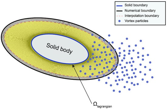
Figure 1.
Domain decomposition of the computational domain for the hybrid solver. The Eulerian mesh extends up to the numerical boundary, which is a short distance away from the solid boundary, while the Lagrangian solver covers the entire computational domain.
2.1. Vortex Particle Method (VPM)
Here, a brief overview of the VPM is presented. For more comprehensive information about this specific method, reference can be made to the analytic description in [6], review paper [7], or the paper that outlines the current hybrid solver, [1].
VPM is a method which belongs to the Lagrangian approach family, where the observer operates within the particle’s frame of reference. The fundamental quantity characterizing the flow conveyed by particles is vorticity, which holds significant relevance in determining the aerodynamic forces acting on bluff bodies. Lagrangian methods, including VPMs, can significantly reduce the numerical diffusion and numerical dispersion that Eulerian solvers introduce. Furthermore, due to the inherent nature of the method, acceleration techniques are widely adopted in VPMs, as the vorticity field originates from the linear solution of the Laplace equation, allowing for efficient parallel solving using Graphics Processing Units (GPUs) [22]. Additionally, Fast Multipole Methods (FMMs), as discussed in [23,24], can significantly enhance computational speed, rendering VPMs a formidable tool for fluid dynamics simulations.
In VPMs, the Navier–Stokes (N-S) equations are written in a velocity–vorticity formulation:
The fluid is discretized into vortex elements, where the total field results from the summation of the induced fields of all these elements. To achieve a smooth representation of the vorticity field, as opposed to the spurious one produced by Dirac distributions, mollified particles are frequently employed. The induced velocity and vorticity fields, utilizing the Gaussian kernel as a smoothing function, are expressed as follows:
The particles are advected and diffused in time and space making use of the Viscous Splitting Algorithm proposed in [25]. The algorithm is characterized by the following equations:
The convection step is resolved utilizing the fourth-order Runge–Kutta integration scheme, while the diffusion process is represented by the Vortex Redistribution Method as proposed in [26]. Further details regarding the Lagrangian solver employed in this context can be located in the primary paper of this hybrid code [1].
2.2. Flowchart of the Hybrid Solver
The two component solvers of the hybrid solver are coupled in a two-way fashion. Initially, in the first step, the Lagrangian particles compute boundary conditions for the numerical boundary (refer to Figure 1) of the Eulerian solver. Subsequently, in the next coupling step, the Eulerian solution is employed to correct the Lagrangian solution within the interpolation region (see Figure 1). Within a given time-step, assuming that both the Eulerian and Lagrangian solutions adequately represent the flow fields, the processes occurring within a single hybrid solver time-step are illustrated in Figure 2.
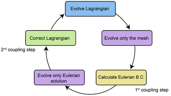
Figure 2.
The flowchart of the steps that are taking place in one hybrid solver time-step.
It has to be mentioned here that these steps are taking place once in each time-step, resulting in weak coupling between the two solvers. The processes governing the evolution of the Eulerian mesh and the evolution of the Eulerian solution are depicted in the same color, as both of them pertain exclusively to the Eulerian solver.
Most of these steps have already been discussed in detail in [1]. The primary distinction lies in the fact that the Eulerian mesh is now in motion. Therefore, before calculating the Eulerian boundary conditions, the Eulerian solver updates its mesh using the prescribed motion specified by the user. It is important to emphasize that Fluid–Structure Interaction (FSI) is not addressed in this context, and special modifications are required in the code to account for such scenarios. Here, the mesh undergoes motion solely based on predefined motion patterns. The mesh is in motion, and consequently the interpolation region moves as well, as illustrated in Figure 3.
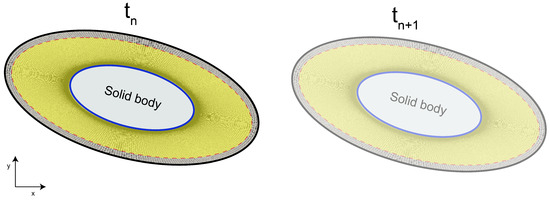
Figure 3.
The mesh is in motion, and along with it, the interpolation region is also in motion. It is important to note that this illustration depicts an exaggerated movement for visualization purposes. In practice, the mesh cannot move to such an extent within a single time-step.
Hence, prior to computing any boundary conditions, the updated coordinates of the Eulerian mesh are exported. Additionally, the data for the new interpolation region are exported, as they are utilized in subsequent correction steps.
2.3. Boundary and Initial Conditions
In the hybrid framework, the Lagrangian particles can calculate the initial and boundary conditions for the Eulerian solver. Specifically, depending on the flow that is simulated, a set of particles can be initialized offering the locations and the strengths of the particles. Using the set of particles and the induced velocity equations (see Equation (3)), the initial velocity field in OpenFOAM can be determined. During the simulation, the particles also determine the boundary conditions for the Eulerian solver. OpenFOAM needs velocity and pressure boundary conditions only, when the turbulence options is disabled. The boundary conditions that are used in OpenFOAM are the following:
- Dirichlet boundary conditions for velocity across the boundary ().
- Neumann boundary conditions for pressure across the boundary ().
The pressure gradient is obtained from the unsteady Bernoulli equation (Equation (7)). Knowing the induced velocity from all the particles, all the terms in the right-hand side (RHS) can be calculated in order to obtain the pressure gradient. These values are assigned at the center of the outer faces.
3. PimpleFOAM Modification
In this project, OpenFOAM v9 [27] is employed as the Eulerian component of the hybrid solver. Specifically, the solver utilized in this context is pimpleFOAM, an incompressible, transient solver capable of accommodating dynamic mesh simulations. pimpleFOAM uses the PIMPLE algorithm [28] for correcting the velocity and pressure fields to enforce the continuity equation. In a standard OpenFOAM case, when the user invokes the pimpleFOAM solver, it triggers a while loop that runs from the initial to the simulation’s end time. The details of this loop’s formulation can be found in Appendix A. However, this particular formulation is not suitable for accommodating the coupling of OpenFOAM with an additional solver, as is the case here. In this hybrid approach, coupling steps must occur immediately before and after each Eulerian step to establish the necessary coupling. Moreover, in the context of a moving mesh, actions need to be taken in the interim. This is because, after the mesh undergoes motion, boundary conditions must be computed for the updated coordinates of the boundary faces.
For this purpose, the original structure of pimpleFOAM is modified, resulting in the creation of a new class-based solver called EulerianPimpleFoam. All the processes within the Eulerian solver are now encapsulated as member functions of this class, providing enhanced control and coordination. In the hybrid solver, at any given time, the Eulerian component can halt its operations, export data, receive new inputs, and establish efficient communication with the Lagrangian solver. This structure facilitates a more organized and flexible interaction between the Eulerian and Lagrangian components. The solver’s structure is visually depicted in Figure 4.
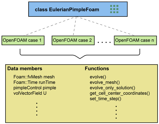
Figure 4.
EulerianPimpleFoam class structure.
Another noteworthy advantage of this solver’s specific structure is its ability to handle multiple OpenFOAM cases simultaneously. Each OpenFOAM case can be instantiated as an object of the class and executed independently. This capability enables the simulation of multi-body scenarios, with Lagrangian particles facilitating interconnections between various Eulerian regions.
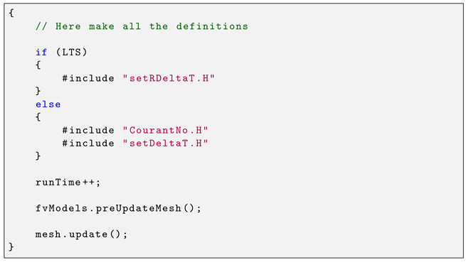
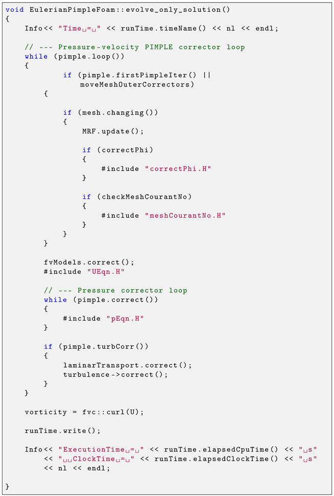
As previously mentioned, to facilitate dynamic mesh simulations within the hybrid framework, the mesh motion and solution evolution need to be separated. Consequently, when conducting a dynamic mesh simulation, the Eulerian evolution comprises two distinct steps: evolve_mesh() and evolve_only_solution() functions. These functions presented in a pseudocode format can be seen in Algorithms 1 and 2. The original codes in the OpenFOAM language format can be seen in Appendix A. It is apparent that, in contrast to the original structure outlined in Appendix B, the mesh is initially updated before proceeding with solution evolution.
| Algorithm 1 The evolve_mesh member function that updates only the mesh of the Eulerian part. | |
| |
|
|
| Algorithm 2 The evolve_only_solution member function that evolves the Eulerian solution without moving the mesh. | |
| |
|
|
| |
|
|
4. Validation
4.1. Validation Cases
Now that the hybrid solver and the modifications to the Eulerian part were discussed, it is time for the validation to be provided. The solver is validated in unbounded cases, meaning that solid boundaries are not present. In all the cases that are presented here, the same Eulerian mesh is used. This mesh, illustrated in Figure 5, is a structured square mesh with an edge length of L, while the distance of the mesh edges to the edges of the interpolation region is denoted as .
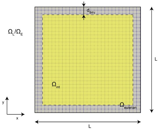
Figure 5.
The geometry and mesh utilized for the validation cases, showcasing the Eulerian domain, the Lagrangian domain, and the interpolation region.
The various cases chosen for validation, as depicted in Figure 6, encompass translational motion, rotational motion, linear oscillation, and multi-motion, which combines linear oscillation and rotation. In each of these cases, a stationary Lamb–Oseen vortex [29] is present within the flow. The Eulerian domain is in relative motion to the vortex, following the specified motion patterns. The Lamb–Oseen vortex is characterized by analytical solutions outlined in the following equations:
where is circumferential velocity, is radial velocity and is vorticity. is the strength of the vortex, t is simulation time, is the time constant (for smooth distribution of the vorticity field), is kinematic viscosity and r is the distance from the core center.
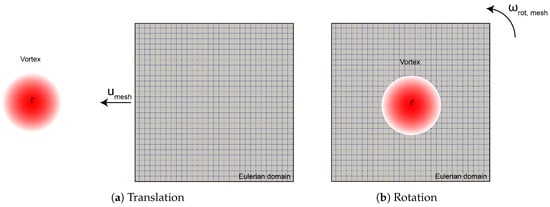
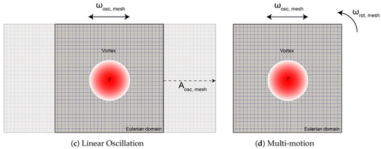
Figure 6.
Validation cases featuring a stationary vortex of strength , with the Eulerian subdomain exhibiting relative motion. The following relative motions are considered: (a) Translation, (b) Rotation, (c) Linear Oscillation, and (d) Linear Oscillation with Rotation (Multi-Motion).
In all cases, comparison is conducted with analytical results. Table 1 provides an overview of geometry and motion parameters for the various cases presented. To ensure a fair comparison among the different motion scenarios, the time-step is adjusted individually in each case to achieve a nearly identical maximum Courant number, which is approximately set to be . Table 2 summarizes the simulation parameters that are consistent across all cases.

Table 1.
Variable parameters associated with domain motion across the different cases.
Table 2.
Simulation parameters for all the moving domain cases.
4.1.1. Translational Motion
The first results to be examined are those of the mesh in translational motion. As depicted in Figure Figure 6a, the vortex initially lies outside the Eulerian domain, with the Eulerian mesh traveling across the vortex in the direction passing through the vortex. Figure 7 displays a comparison of the x and y components of the velocity field for both the analytical and hybrid solutions within the same contour. The contour is divided, with the upper part corresponding to the analytical solution and the lower part to the hybrid solution. The red dashed box denotes the position of the Eulerian mesh at the corresponding time instance. Evidently, there is a substantial agreement between the two solutions. To assess the error between the two solutions in the vorticity field, Figure 8a illustrates the relative error in the vorticity field for the two solutions. The error is computed in a manner that prevents division by very small numbers in regions where vorticity is close to zero, as described in Equation (10).
where is the relative vorticity error at time t, is hybrid vorticity and is analytical vorticity. It is noteworthy that, for all time instances, the error remains below . The error is negligible when the Eulerian domain has not reached the vortex, and there is a sudden increase when it crosses the vortex. This increase in the error is primarily due to discretization and interpolation from the Eulerian field to the Lagrangian field. Figure 8b presents a comparison of the vorticity error for six different cases within the translational domain. These cases employ various mesh sizes and particle spacings to demonstrate the convergence of the solution as mesh size increases or particle spacing decreases. In all the results provided, the finest mesh size and particle spacing are used, specifically cells and m.
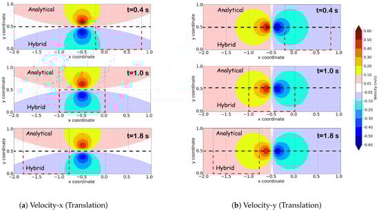
Figure 7.
Comparison of the velocity field between the analytical (top) and hybrid (bottom) solutions for the translational case. The x-component of velocity is depicted on the left, while the y-component is shown on the right. The analytical and hybrid solutions are separated by a black dashed line [---] and the Eulerian domain at the corresponding time instance is defined by a red rectangle,  . The dashed box extends to the analytical part only for visualization purposes and is illustrated with a thinner green line.
. The dashed box extends to the analytical part only for visualization purposes and is illustrated with a thinner green line.
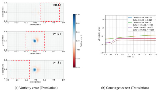
Figure 8.
On the left, the relative error of the vorticity field between the hybrid and the analytical solution for the translational case is illustrated. The Eulerian domain at the corresponding time instance is defined by a red rectangle, . On the right, the convergence test for the mesh size and the particles’ spacing is depicted.
. On the right, the convergence test for the mesh size and the particles’ spacing is depicted.
4.1.2. Rotation
The second validation case involves the pure rotation of the Eulerian domain, as depicted in Figure 6b. This time, the vortex is situated within the Eulerian domain, and the domain initiates a rotational motion around its center, coinciding with the center of the vortex’s core. In this and subsequent cases, only the vorticity field and the associated error are presented. Figure 9b illustrates a noteworthy agreement in the vorticity field between analytical and hybrid solutions. Specifically, the maximum errors are constrained to , and this error is present from the beginning of the simulation due to discretization. As the vortex neither enters nor exits the Eulerian domain in this case, no additional errors are introduced.
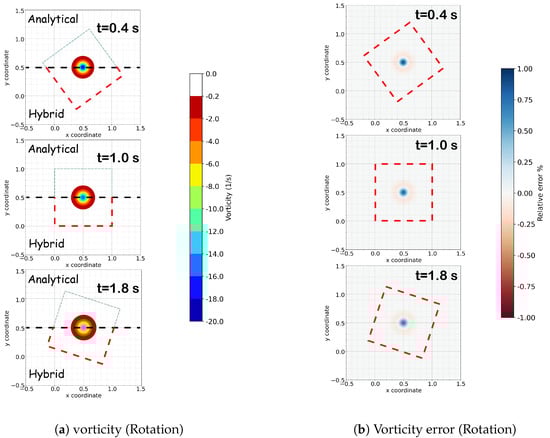
Figure 9.
On the left is the comparison of the vorticity field between the analytical (top) and hybrid (bottom) solutions for the rotational case. The analytical and hybrid solutions are separated by a black dashed line [---] and the Eulerian domain at the corresponding time instance is defined by a red rectangle, . The dashed box extends to the analytical part only for visualization purposes and is illustrated with a thinner green line. On the right, the relative error of the vorticity field between the hybrid and analytical solutions for the rotational case is illustrated.
. The dashed box extends to the analytical part only for visualization purposes and is illustrated with a thinner green line. On the right, the relative error of the vorticity field between the hybrid and analytical solutions for the rotational case is illustrated.
4.1.3. Linear Oscillation
The third validation case involves the oscillation of the Eulerian mesh, as it can be seen in Figure 6c. The domain moves up to the point that the vortex is entirely outside of the Eulerian mesh, and when it reaches the peak of its oscillation, it returns to its initial position. In Figure 10, it is evident that the vorticity field between the analytical solution and the hybrid solution demonstrates a strong agreement. Regarding errors, all errors remain below . Notably, in this case, where the vortex is initially within the Eulerian domain, the interpolation error is present from the start of the simulation, and it increases by approximately when the Eulerian domain encompasses the vortex for the second time.
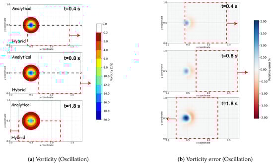
Figure 10.
On the left is the comparison of the vorticity field between the analytical (top) and hybrid (bottom) solutions for the linear oscillation case. The analytical and hybrid solutions are separated by a black dashed line [---] and the Eulerian domain at the corresponding time instance is defined by a red rectangle, . The dashed box extends to the analytical part only for visualization purposes and is illustrated with a thinner green line. On the right, the relative error of the vorticity field between the hybrid and analytical solutions for the linear oscillation case is illustrated.
. The dashed box extends to the analytical part only for visualization purposes and is illustrated with a thinner green line. On the right, the relative error of the vorticity field between the hybrid and analytical solutions for the linear oscillation case is illustrated.
4.1.4. Multi-Motion
In the last validation case, the Eulerian mesh performs a more complex motion pattern. Specifically, the vortex is initially located at the center of the Eulerian mesh, and this starts a combined linear oscillation in the x axis and a rotation around point . This combined motion causes the Eulerian domain to pass through the vortex twice. Figure 11 shows a great agreement of the vorticity field between the hybrid and analytical solutions, while the vorticity error presented in Figure 11b is always lower than . An initial error around is present since the start of the simulation, and it grows to when the Eulerian mesh passes through the vortex for the second time.
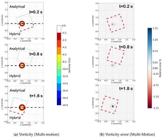
Figure 11.
On the left is the comparison of the vorticity field between the analytical (top) and hybrid (bottom) solutions for the multi-motion case. The analytical and hybrid solutions are separated by a black dashed line [---] and the Eulerian domain at the corresponding time instance is defined by a red rectangle, . The dashed box extends to the analytical part only for visualization purposes and is illustrated with a thinner green line. On the right, the relative error of the vorticity field between the hybrid and the analytical solution for the multi-motion case is illustrated.
. The dashed box extends to the analytical part only for visualization purposes and is illustrated with a thinner green line. On the right, the relative error of the vorticity field between the hybrid and the analytical solution for the multi-motion case is illustrated.
The final result presented here is Figure 12. In this figure, both the vorticity error and the circulation deficit are provided for each individual case. Figure 12a demonstrates that, for all cases, the typical error remains at approximately . It is notable that there is a slight increase in vorticity when the vortex enters the Eulerian domain, but this increase remains minimal. Figure 12b reveals that, for every case, the circulation of the flow can be conserved up to three significant digits.
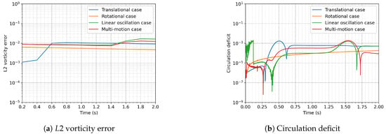
Figure 12.
On the left is the vorticity error for all the different scenarios that are presented. On the right, the circulation deficit for each case is illustrated.
4.2. Conclusions
The results presented above demonstrate that the solver can effectively handle a range of mesh motions. In all the cases, the vorticity errors are approximately , while the maximum errors in each case remain below . These errors are primarily due to discretization and can be further reduced, as illustrated in Figure 8b. A slight increase in the error is observed when the vortex enters the Eulerian mesh, but this increase is not substantial and falls within acceptable limits. No specific mesh motion appears to generate significantly higher errors, indicating that the solver can consistently and accurately handle various mesh motions.
5. Summary and Discussion
This study focuses on dynamic mesh simulations within OpenFOAM, specifically in a hybrid Eulerian–Lagrangian framework. This paper expands on the previously published work of our team [1] and extends the solver’s capability in simulating dynamic meshes. A modification of the original pimpleFOAM solver in OpenFOAM v9 is undertaken to make it compatible with coupling, as coupling steps are essential within an OpenFOAM time-step. The dynamic mesh movement applied here is solid-motion, typically used when the outer patches represent walls, as seen in scenarios like sloshing tanks. In this method, Lagrangian particles are employed to compute boundary conditions for the Eulerian field, rendering it suitable for open-boundary cases. The solver undergoes testing with different types of motion to validate its performance across various scenarios.
The results presented in the previous section indicate that the solver effectively handles diverse mesh motions and exhibits excellent agreement with the analytical solution. This demonstrates the suitability of the proposed method for conducting dynamic mesh simulations in this manner, paving the way for the application of the hybrid solver in more complex aerodynamic cases, including scenarios like oscillating cylinders and pitching airfoils.
Author Contributions
R.P.: Conceptualization, Software development, Validation, Methodology, Data curation, Visualization, Interpretation, Writing—Original draft. C.S.F.: Conceptualization, Supervision, Project administration, Reviewing and Editing of draft. A.v.Z.: Conceptualization, Supervision, Project administration, Reviewing and Editing of draft. C.F.B.: Conceptualization, Software development, Reviewing and Editing of draft. All authors have read and agreed to the published version of the manuscript.
Funding
This research received no external funding.
Data Availability Statement
No new data were created or analyzed in this study. Data sharing is not applicable to this article.
Acknowledgments
The authors acknowledge the use of OpenAI’s ChatGPT 3.5 AI tool which was used for grammar and spell-check purposes in the abstract and introduction sections of the paper in order to increase readability.
Conflicts of Interest
The authors declare that they have no known competing financial interests or personal relationships that could have appeared to influence the work reported in this paper.
Appendix A
 |
| Listing A1. The evolve_mesh member function that updates only the mesh of the Eulerian part. |
 |
| Listing A2. The evolve_only_solution member function that evolves the Eulerian solution without moving the mesh. |
Appendix B
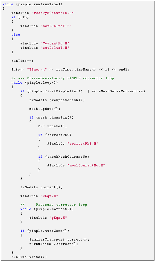 |
| Listing A3. The original pimpleFOAM solver is OpenFOAM v9. |
References
- Pasolari, R.; Ferreira, C.; van Zuijlen, A. Coupling of OpenFOAM with a Lagrangian vortex particle method for external aerodynamic simulations. Phys. Fluids 2023, 35, 107115. [Google Scholar] [CrossRef]
- Papadakis, G.; Voutsinas, S.G. In view of accelerating CFD simulations through coupling with vortex particle approximations. J. Phys. Conf. Ser. 2014, 524, 012126. [Google Scholar] [CrossRef]
- Papadakis, G.; Voutsinas, S.G. A strongly coupled Eulerian Lagrangian method verified in 2D external compressible flows. Comput. Fluids 2019, 195, 104325. [Google Scholar] [CrossRef]
- Billuart, P.; Duponcheel, M.; Winckelmans, G.; Chatelain, P. A weak coupling between a near-wall Eulerian solver and a Vortex Particle-Mesh method for the efficient simulation of 2D external flows. J. Comput. Phys. 2023, 473, 111726. [Google Scholar] [CrossRef]
- Golas, A.; Narain, R.; Sewall, J.; Krajcevski, P.; Dubey, P.; Lin, M. Large-scale fluid simulation using velocity-vorticity domain decomposition. ACM Trans. Graph. 2012, 31, 1–10. [Google Scholar] [CrossRef]
- Cottet, G.H.; Koumoutsakos, P. Vortex Methods—Theory and Practice; Cambridge University Press: Cambridge, UK, 2000. [Google Scholar]
- Mimeau, C.; Mortazavi, I. A review of vortex methods and their applications: From creation to recent advances. Fluids 2021, 6, 68. [Google Scholar] [CrossRef]
- Park, Y.M.; Jee, S. Numerical study on interactional aerodynamics of a quadcopter in hover with overset mesh in OpenFOAM. Phys. Fluids 2023, 35, 085138. [Google Scholar] [CrossRef]
- Alletto, M. Comparison of Overset Mesh with Morphing Mesh: Flow Over a Forced Oscillating and Freely Oscillating 2D Cylinder. OpenFOAM® J. 2022, 2, 13–30. [Google Scholar] [CrossRef]
- Wu, Y.; Dai, Y.; Yang, C. Time-Delayed Active Control of Stall Flutter for an Airfoil via Camber Morphing. AIAA J. 2022, 60, 5723–5734. [Google Scholar] [CrossRef]
- feng Tan, J.; wen Wang, H. Simulating unsteady aerodynamics of helicopter rotor with panel/viscous vortex particle method. Aerosp. Sci. Technol. 2013, 30, 255–268. [Google Scholar] [CrossRef]
- Papadakis, G.; Riziotis, V.A.; Voutsinas, S.G. A hybrid Lagrangian–Eulerian flow solver applied to elastically mounted cylinders in tandem arrangement. J. Fluids Struct. 2022, 113, 103686. [Google Scholar] [CrossRef]
- Stock, M.J.; Gharakhani, A.; Stone, C.P. Modeling rotor wakes with a hybrid OVERFLOW-vortex method on a GPU cluster. In Proceedings of the 28th AIAA Applied Aerodynamics Conference, Chicago, IL, USA, 28 June–1 July 2010; Volume 1. [Google Scholar] [CrossRef]
- Shi, Y.; Xu, G.; Wei, P. Rotor wake and flow analysis using a coupled Eulerian-Lagrangian method. Eng. Appl. Comput. Fluid Mech. 2016, 10, 384–402. [Google Scholar] [CrossRef]
- Weller, H.G.; Tabor, G.; Jasak, H.; Fureby, C. A tensorial approach to computational continuum mechanics using object-oriented techniques. Comput. Phys. 1998, 12, 620–631. [Google Scholar] [CrossRef]
- Lukashin, P.; Melnikova, V.; Shcheglov, G.; Strijhak, S. Using Open Source Software for Solving Aeroelasticity Case for Wind Turbine Blade. In Proceedings of the 6th European Conference on Computational Mechanics (Solids, Structures and Coupled Problems) (ECCM 6) and the 7th European Conference on Computational Fluid Dynamics (ECFD 7), Glasgow, UK, 11–15 June 2018; pp. 573–584. [Google Scholar]
- Pradhan, A.; Arif, M.R.; Afzal, M.S.; Gazi, A.H. On the origin of forces in the wake of an elliptical cylinder at low Reynolds number. Environ. Fluid Mech. 2022, 22, 1307–1331. [Google Scholar] [CrossRef]
- Li, Y.L.; Zhu, R.C.; Miao, G.P.; Ju, F.A.N. Simulation of tank sloshing based on OpenFOAM and coupling with ship motions in time domain. J. Hydrodyn. Ser. B 2012, 24, 450–457. [Google Scholar] [CrossRef]
- Chen, Y.; Xue, M.A. Numerical Simulation of Liquid Sloshing with Different Filling Levels Using OpenFOAM and Experimental Validation. Water 2018, 10, 1752. [Google Scholar] [CrossRef]
- Daeninck, G. Developments in Hybrid Approaches: Vortex Method with Known Separation Location. Ph.D. Thesis, UCLouvain, Ottignies-Louvain-la-Neuve, Belgium, 2006. [Google Scholar]
- Palha, A.; Manickathan, L.; Ferreira, C.S.; van Bussel, G. A hybrid Eulerian-Lagrangian flow solver. arXiv 2015, arXiv:1505.03368. [Google Scholar]
- Hu, Q.; Gumerov, N.A.; Duraiswami, R. GPU accelerated fast multipole methods for vortex particle simulation. Comput. Fluids 2013, 88, 857–865. [Google Scholar] [CrossRef]
- Goude, A.; Engblom, S. Adaptive fast multipole methods on the GPU. J. Supercomput. 2013, 63, 897–918. [Google Scholar] [CrossRef]
- Engblom, S. On well-separated sets and fast multipole methods. Appl. Numer. Math. 2011, 61, 1096–1102. [Google Scholar] [CrossRef]
- Chorin, A.J. Numerical Study of Slightly Viscous Flow. J. Fluid Mech. 1973, 57, 785–796. [Google Scholar] [CrossRef]
- Tutty, O.R. A Simple Redistribution Vortex Method (with Accurate Body Forces). arXiv 2010, arXiv:1009.0166. [Google Scholar]
- OpenFOAM v9. Available online: https://openfoam.org/version/9/ (accessed on 12 February 2024).
- OpenFOAM guide/The PIMPLE algorithm in OpenFOAM. Available online: https://openfoamwiki.net/index.php/OpenFOAM_guide/The_PIMPLE_algorithm_in_OpenFOAM (accessed on 12 February 2024).
- Lamb, H. Hydrodynamics, 6th ed.; Cambridge University Press: Cambridge, UK, 1993. [Google Scholar]
Disclaimer/Publisher’s Note: The statements, opinions and data contained in all publications are solely those of the individual author(s) and contributor(s) and not of MDPI and/or the editor(s). MDPI and/or the editor(s) disclaim responsibility for any injury to people or property resulting from any ideas, methods, instructions or products referred to in the content. |
© 2024 by the authors. Licensee MDPI, Basel, Switzerland. This article is an open access article distributed under the terms and conditions of the Creative Commons Attribution (CC BY) license (https://creativecommons.org/licenses/by/4.0/).