Abstract
Kelvin–Helmholtz instability has been studied extensively in 2D. This study attempts to address the influence of turbulent flow and cross perturbation on the growth rate of the instability and the development of mixing layers in 3D by means of direct numerical simulation. Two perfect gases are considered to be working fluids moving as opposite streams, inducing shear instability at the interface between the fluids and resulting in Kelvin–Helmholtz instability. The results show that cross perturbation affects the instability by increasing the amplitude growth while adding turbulence has almost no effect on the amplitude growth. Furthermore, by increasing the turbulence intensity, a more distinct presence of the inner flow can be seen in the mixing layer of the two phases, and the presence of turbulence expands the range of high-frequency motion significantly due to turbulence structures. The results give a basis for which 3D Kelvin–Helmholtz phenomena should be further investigated using numerical simulation for predictive modeling, beyond the use of simplified 2D theoretical models.
1. Introduction
Kelvin–Helmholtz instability (KHI) is a classic fluid dynamical problem relevant to many industrial applications and natural phenomena, such as interfacial instability of two flow streams in fuel injection systems, turbulence transition, and breaking waves in the ocean. The phenomena was first described by Helmholtz in 1868 [1]. Kelvin–Helmholtz instability was first studied through experiments in the late 1960s [2]. This instability was then explored assuming predominantly 2D behavior, linearizing the problem using linear stability theory [3,4]. Conventionally, the development of the interfacial wave is addressed through a linearized theory of small perturbations of the two-dimensional base flow. The linear stability theory that leads to the theoretical prediction of the most unstable frequency was first carried out assuming inviscid flows [5]. This theory was developed for the inviscid case, showing that the introduction of body forces such as gravity and surface tension tend to dampen instabilities, giving a minimum wave number for which instability will result. This is described in depth in the next section.
The theory was then extended to viscous flow. Some early work in KHI was carried out by Ozgen and others which described the effects of viscosity on the stability characteristics, as well as the effects of gravity and surface tension (Praturi et al. [6], Ozgen et al. [7], Sivadas et al. [8], Otto et al. [9], and Obergaulinger [10]). Comparison of theory to experiments was continued with Yoshikawa for large contrast in viscosity [11]. Experimental results were compared to linear stability theory by Matas in 2011 [5]. Experimental analysis of KHI was continued by Karabyoglu and Petrarolo in engineering applications of shear flow [12,13,14]. While it is important to characterize the viscous effects, this study focuses on the contribution of the initial disturbances in the inviscid case in order to compare more directly to linear stability theory.
With the rise of computational power and numerical simulations, direct numerical simulations (DNSs) of interfacial instabilities became viable. Direct numerical simulation has been a great tool in furthering the understanding of this instability phenomenon. Lee and Kim studied KHI with a 2D DNS using a phase field [15]. The use of DNS for solving KHI is explored in Atmakidis, which validates different DNS methods against linear stability theory [16]. Zhang in 2018 used a 2D DNS to present the effect of three fluid layers on KHI [17]. A parametric study of KHI behavior was also developed using 2D simulation results [18]. Recent simulations have provided high-resolution details of the interfacial instability development, the interaction between the interfacial wave and the gas stream, and the formation of the two-phase mixing layer [19]. Here, the ’mixing layer’ is defined as the region near the fluid interface where one fluid is thoroughly interspersed with the other fluid [20]. Therefore, it is mechanically mixed, and no diffusion is assumed between fluids.
After validation of KHI simulations in 2D, this phenomenon can be investigated in more detail in 3D. Linear stability theory deals with simplifications that restrict it to a 2D problem, while turbulence is a predominantly 3D phenomenon. Rogers and Moser 1991 [21], Martinez 2006 [22], Soetrisno 1990 [23], and Wang 2016 [24] analyzed 3D KHI simulations. The study of turbulence in relation to KHI has only recently been explored [20,25].
Kelvin–Helmholtz instability occurs when two parallel fluid streams have a difference in velocities, which induces shear instability at the interface between the fluids. This instability creates roll-up structures that eventually dissipate due to turbulent effects. Although the simple Kelvin–Helmholtz instability behavior has long been an active field of study, comparatively less is known about how these Kelvin–Helmholtz instability structures can be changed by modifying initial flow conditions in three dimensions. This would be helpful in developing predictive modeling of such instabilities in turbulent conditions. Other parametric studies have been conducted on the effects of Kelvin–Helmholtz instability, especially in 2D [26], while experimental and simulation studies have been conducted over the years to understand the roll-up structures that develop as a result [12,13,14]. However, the interest of this study lies in the initiation of Kelvin–Helmholtz instability and which parameters, such as interface shape and velocity profiles, can change the development of Kelvin–Helmholtz instability features in three dimensions; this can only be studied with DNSs. This would be useful in predictive models since the 2D theoretical description might not correctly describe the intricacies of instability development with the addition of cross-wise disturbances. Parametric studies tend to focus on laminar cases, while the application of Kelvin–Helmholtz shear instability in a turbulent environment can be complex compared to the 2D theory. This study looks at the addition of three-dimensional interface shape changes as well as the addition of turbulence in the stream-wise driving velocity. In this study, a DNS is conducted to evaluate the effect of cross perturbation in combination with turbulent structures on the instability mechanism and the mixing layer between two streams. Here, two perfect gases are considered as working fluids moving as opposite streams.
2. Linear Stability Theory
Linear stability theory for Kelvin–Helmholtz was first introduced by Chandrasekhar [3] and is also explained by Drazin [4]. The theory is developed assuming incompressible, inviscid flow restricted to velocity only in the x-direction and assuming sinusoidal perturbation of the interface. Linearization of the equations assumes a small initial perturbation, with small defined as . Using the method of normal nodes, the solution is therefore assumed to have the following exponential form:
where y is the height of the interface from the center line, is the initial amplitude of the sinusoidal perturbation of the interface, is the frequency and comes from the roots of the characteristic equation, and k is the wave number.
where the first term in the square root is the contribution due to shear velocity, the second is the contribution of gravity g, and the third term is the contribution of surface tension . Gravity and surface tension are stabilizing, so a minimum wave number, , must be exceeded for the instability to occur. Conversely, this means that for the inviscid case neglecting body forces, the result should always be unstable.
The exponential growth of the initial instability is given by the real part of the equation:
with the amplitude for the Kelvin–Helmholtz simulations in this study given by the following expression:
This solution only holds at the very early stages of the simulation when the sinusoidal shape of the interface is maintained. As soon as cresting of the waves occurs, the amplitude growth slows down, and linear theory no longer applies. This analysis, however, gives a quantifiable way to assess whether the Kelvin–Helmholtz simulations are valid for the VOF solver.
3. Isotropic Turbulence
To explore the influence of a turbulent initial velocity field on the growth of Kelvin–Helmholtz instability, the 3D case is given a shear velocity with the addition of isotropic synthetic turbulence of the stream-wise velocity. This turbulent field was generated using the Kraichnan method presented by Saad [27]. This method initiates the velocity in each cell using a parsed series of 5000 terms. The fluctuation in the x-direction velocity is given by the following equation:
where is a scaling constant, is the wave number where energy is maximum, and is the root mean square value of the velocity fluctuations and is adjusted depending on the desired turbulence intensity.
where L is the integral length scale, defined by , with , and is the kinematic viscosity of the fluid.
For the simulations here, the values used are , , and .
4. Methodology and Simulation Domain
A compressible volume of fluid (VOF) method is used to solve the Euler Equations, neglecting viscous diffusion.
where is the source term vector, p is pressure, and H is total enthalpy defined by . This advects the conserved values (), in which represents the volume fraction of the gas phase (or the fluid of interest in a 2-gas case), is the density of the gas phase in the domain, is the density of the bulk fluid in any cell within the domain, E is total energy, and is the velocity within the domain. The VOF code is part of an open-source software ABLATE, developed to conduct DNS simulations of the combustion process inside hybrid rocket motors [28]. It uses explicit solvers and a stratified flow model to improve scalability, as this allows for a multiphase solution without the reconstruction of the interface. The code is validated in multiple research papers [29,30].
The case considered here is an inviscid shear-driven instability due to the velocity difference between two streams. The coordinate system used is a Cartesian system, with the flow directed in the x-direction, the interface height measured in the y-direction, and the depth defined as the z-direction, as shown in Figure 1. The conventional perturbation is in the y-direction, while the cross perturbation is in the z-direction. The initial interface for the classic Kelvin–Helmholtz case is given by
where the second sinusoidal term acts as the additional cross perturbation. The resulting interface shape is shown in Figure 2. The wave amplitude is measured as half the vertical distance from wave crest to trough, thus the initial amplitude m in the above case, with wave number . Both fluids are perfect gases (, ). The density in the inner region is = 1 kg/ and that of the outer region is = 2 kg/, with uniform pressure p = 2.5 Pa everywhere. The velocity is m/s in the inner region and m/s in the outer region. The velocity of m/s was chosen so that the case would be in the regime for instability. According to linear stability theory, for inviscid cases with no additional body forces, any wave number will produce instability, and the regime is always unstable. However, due to numerical diffusion caused by the mesh resolution, a sufficient velocity is necessary for the Kelvin–Helmholtz instability to develop. The 3D domain size is m with a mesh of , in streamwise, vertical, and spanwise directions, respectively. Periodic boundary conditions are applied to all boundaries of the domain. In the cases with turbulent initial conditions, an isotropic synthetic turbulent field is generated using synthetic isotropic turbulence of the Kraichnan method [27], with intensities of and , where . All cases are simulated until s in order to see the breakdown of the interface into turbulence.
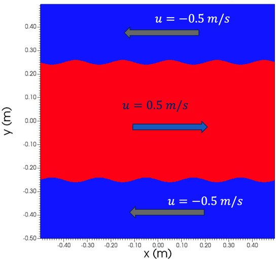
Figure 1.
Problem setup for Kelvin-Helmholtz instability.
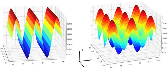
Figure 2.
Initial interface contour for (left) no cross-perturbation case vs. (right) with cross-perturbation case.
Grid Convergence Study
In order to evaluate the sufficiency of grid sizes to capture the features of the instability at the interface, a convergence study is conducted as the mesh size is increased on a domain of 0.2 m × 1 m × 0.2 m; three computations are conducted on a sequence of three meshes with various grid resolutions: coarse, medium, and fine. These are defined in Table 1. For the generated isotropic turbulence, the integral length scale is , with being the wave number where energy is maximum in the energy spectrum [27]. Here the isotropic turbulence is generated with an integral length scale of m, which is significantly larger than the coarse grid size. Therefore, all three grids resolve the integral length scale. Figure 3 shows the interface contours for various meshes, taken at s. As the contours indicate, the numerical solution tends toward a unique shape as the grid resolution is increased. It is apparent that the coarse grid does not resolve the details of the interface where the curvature at the interface begins to develop, m. In contrast, the medium and fine meshes resolve curvature adequately; therefore, the medium grid is selected to conduct simulations.

Table 1.
Grid sizes for KHI convergence.
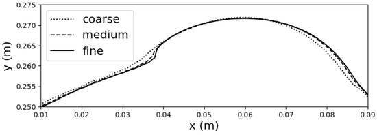
Figure 3.
Interface contour for various mesh resolutions at t = 0.1 s.
5. Results
Figure 4 shows the 2D cross section of the 3D simulation results in the x-y plane (). This shows the expected roll-up behavior of the sinusoidal initial interface, forming wave crests at s and continuing to swirl at s. These swirling structures roll onto themselves at s, as shown in the bottom left image in Figure 5. These later diffuse and break up at s and s, as shown in the bottom center and bottom right images in Figure 5. The amplitude as well as kinetic energy was measured at each time step to compare the results between cases. Q-criterion contours were also shown for s to compare the swirling behavior between the cases with and without cross perturbation.
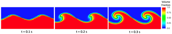
Figure 4.
Volume fraction for I = 0 case (left) linear theory zone, (center) beginning of cresting, (right) swirling. Black line is contour at .
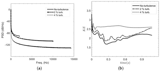
Figure 5.
(a) Power spectral density of density fluctuations vs. frequency and (b) time evolution of kinetic energy for various turbulence intensity.
5.1. Effect of Cross Perturbation
Figure 6 shows the growth of wave amplitudes over time for one case with and one without cross perturbation, as well as cases with cross perturbation and the addition of and turbulence intensity in the initial streamwise velocity. The initial amplitude in the domain is m. As predicted by linear stability theory [3,4], the initial growth is exponential, from to s. This is the time at which the wave begins to crest and linear theory breaks down, after which growth decelerates and the transition to turbulence begins, as shown in Figure 4. The definition of ’mixing’ as stated by Ling et al. [20] is adopted which refers to the immiscible fluids creating a layer near the interface where one fluid is dispersed into the other fluid phase. At s, the wave enters the nonlinear phase. The momentum drives the swirling of the vortex instead of contributing to amplitude growth, and eventually, the two-phase mixing layer starts to develop. As evident from the difference in slopes in Figure 6, cross perturbation affects the instability by increasing the amplitude growth, while adding turbulence has almost no effect on the amplitude growth.
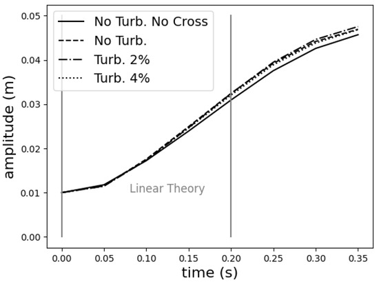
Figure 6.
Amplitude of interface over time.
To better understand the mechanism of instability in the presence of cross perturbation, iso-surfaces of the Q-criterion are plotted in Figure 7 colored by vorticity in the spanwise direction, with units [rad/s]. Note that vorticity is negligible in other directions. The Q-criterion allows one to visualize a vortex, and it is defined as where and S are rotation and strain rate tensors, respectively. The counter-rotating vortices of upper and lower waves are apparent from the red and blue contours of spanwise vorticity, respectively. The roll wave structures are thickened especially near the peak of waves, leading to an early initiation of instability due to cross perturbation. On the other hand, the contours reveal that the vorticity magnitude is decreased compared to the no cross-perturbation case. This could be due to the increased spanwise convection caused by the cross-stream, which also stretches the vortices. The spanwise perturbation also seems to break up the tip of roll-up vortices into multiple edges. Overall, the structures are strongly affected by cross perturbation, leading to the initiation of instability.
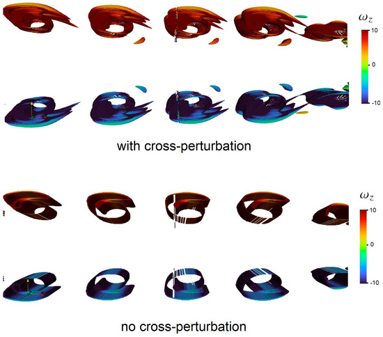
Figure 7.
Q-criterion threshold for cases without turbulence at t = 0.5 s.
5.2. Effect of Turbulence
To evaluate the effect of initial turbulence intensity on the interfacial waves, the contours of volume fraction between two gasses are plotted in Figure 8. The turbulence does not affect the initial roll-up ( s); however, the initial development of mixing at s shows the presence of the inner phase in the mixing is intensified as the turbulence intensity increases. As stated before, the ’mixing layer’ is defined as the region near the fluid interface where one fluid is thoroughly interspersed with the other fluid. Consequently, in the mixing layer at s, a distinct fraction of the inner gas appears as shown in the boxed regions. Note that the shown boxed regions consist of about cells at s and about cells at s, which are significantly resolved compared to the integral length scale, m. Therefore, the intensified colors of the volume fraction are clearly due to the presence of turbulent structures. By increasing the turbulence intensity from to , a more distinct presence of the inner flow can be seen in the mixing layer of the two phases.
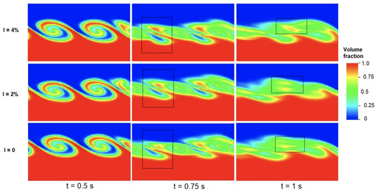
Figure 8.
Contours of volume fraction for various turbulence intensity at different times.
These observations are the motivation for evaluating the power spectral density (PSD) of density fluctuations in the mixing layer, which describes the power of fluctuations as a function of frequency [31]. The probe is located along the initial sinusoid, which develops into the center of one of the vortices and eventually positions inside the layer of mixing fluids. As Figure 5a shows, without turbulence, the spectra are limited to low-frequency motions due to extraction and contractions in the mixing layer. However, turbulence expands the range of high-frequency motions significantly due to turbulence structures, as shown in Figure 5a. In addition, it is apparent that the magnitude of the power spectra increases with turbulence intensity. Figure 5b shows the time evolution of the kinetic energy, , where and where u, v, and w are components of velocity fluctuation in the x, y, and z directions, respectively At s, the kinetic energy values drop to a local minimum because the Kelvin–Helmholtz’s billow structure is partly destroyed, as was also observed by Liu et al. [25]. Then, increases, suggesting the emergence of turbulence. There is a slight increase in the magnitude of with an intensity of compared to the no turbulence case. The evolution, however, is higher for the turbulence intensity of , while it is at a steady rate contrary to the no turbulence and cases. This could be due to higher values of the turbulent kinetic energy, , associated with the turbulent stage of the flow evolution for .
6. Discussion
The effects of cross perturbation and turbulence intensity in the initial conditions are evaluated for shear-driven two-phase Kelvin–Helmholtz instability to characterize their effect on the development of the mixing layer. The appearance of turbulent structures in the gas stream near the interface influences the shape of the interfacial wave over time. This suggests the combined impact of cross perturbation and variation in the velocity field may influence the interface shape in three dimensions over time, deviating from the two-dimensional theoretical models. This is significant in exposing the need for a more detailed parametric study of 3D effects to properly model shear instability for future high-performance simulations. The results show that cross perturbation affects the instability by increasing the amplitude growth while adding turbulence has almost no effect on the amplitude growth. Linear stability theory explains that the addition of vorticity in the initial flow field should not affect the stability in the inviscid case [4], therefore the results found here agree with the theory. The significance is the change in amplitude growth rate caused by the cross perturbation in the initial interface. If these instability growth rates are affected by the initial conditions in 3D, the accuracy of solutions to real-world problems can be significantly improved if more research is conducted on the trends found in varying the interface contour in the z-direction.
Another observation made is by increasing the turbulence intensity a more distinct presence of the inner flow can be seen in the mixing layer of the two phases. Analysis of PSD reveals that the presence of turbulence expands the range of high-frequency motion significantly due to turbulence structures. The evolution of kinetic energy shows a slight increase as the turbulence intensity is increased. This study can be extended to explore how variations in the initial perturbation modify the interface instability process. As simulations are becoming more prevalent and detailed, it would be helpful to break down the individual phenomena in these flows to have better parametric controls on the initial conditions. Continued study of Kelvin–Helmholtz instability with the theory extended to 3D would be a rich resource for future model development for highly accurate DNSs.
Author Contributions
Conceptualization, M.S., J.C. and R.Z.; methodology, M.S. and R.Z.; software, M.S.; validation, M.S. and R.Z.; formal analysis, M.S. and R.Z.; writing—original draft preparation, M.S.; writing—review and editing, J.C.; visualization, M.S. and R.Z.; project administration, J.C.; funding acquisition, J.C. All authors have read and agreed to the published version of the manuscript.
Funding
This research was funded by the United States Department of Energy’s (DoE) National Nuclear Security Administration (NNSA) under the Predictive Science Academic Alliance Program III (PSAAP III) at the University at Buffalo, contract number DE-NA0003961.
Data Availability Statement
Data related to this study is available upon request to the corresponding author.
Conflicts of Interest
The authors declare no conflicts of interest. The funders had no role in the design of this study; in the collection, analyses, or interpretation of data; in the writing of the manuscript; or in the decision to publish the results.
Abbreviations
The following abbreviations are used in this manuscript:
| MDPI | Multidisciplinary Digital Publishing Institute |
| KHI | Kelvin–Helmholtz Instability |
| DNS | Direct Numerical Simulation |
| PSD | Power Spectral Density |
References
- Helmholtz, H. On discontinuous movements of fluids. Phil. Mag. 1868, 36, 337–346. [Google Scholar] [CrossRef]
- Thorpe, S.A. Experiments on the instability of stratified shear flows: Immiscible fluids. J. Fluid Mech. 1969, 39, 25–48. [Google Scholar] [CrossRef]
- Chandrasekhar, S. Hydrodynamic and Hydromagnetic Stability; Oxford Uuniversity Press: Oxford, UK, 1961. [Google Scholar]
- Drazin, P.G. Introduction to Hydrodynamic Stability; Cambridge University Press: Cambridge, UK, 2002. [Google Scholar] [CrossRef]
- Matas, J.P.; Marty, S.; Cartellier, A. Experimental and Analytical Study of the Shear Instability of a Gas-Liquid Mixing Layer. Phys. Fluids 2011, 23, 094112. [Google Scholar] [CrossRef]
- Praturi, D.S.; Girimaji, S.S. Magnetic-Internal-Kinetic Energy Interactions in High-Speed Turbulent Magnetohydrodynamic Jets. J. Fluids Eng. 2020, 142, 101213. [Google Scholar] [CrossRef]
- Özgen, S.; Degrez, G.; Sarma, G.S.R. Two-Fluid Boundary Layer Stability. Phys. Fluids 1998, 10, 2746–2757. [Google Scholar] [CrossRef]
- Sivadas, V.; Karthick, S.; Balaji, K. Symmetric and Asymmetric Disturbances in the Rayleigh Zone of an Air-Assisted Liquid Sheet: Theoretical and Experimental Analysis. J. Fluids Eng. 2020, 142, 071302. [Google Scholar] [CrossRef]
- Otto, T.; Rossi, M.; Boeck, T. Viscous Instability of a Sheared Liquid-Gas Interface: Dependence on Fluid Properties and Basic Velocity Profile. Phys. Fluids 2013, 25, 032103. [Google Scholar] [CrossRef]
- Obergaulinger, M.; Aloy, M. Numerical viscosity in simulations of the two- dimensional Kelvin-Helmholtz instability. In Proceedings of the 14th Numerical Modeling of Space Plasma Flows 2020, Paris, France, 1–5 July 2020; Volume 1623, p. 012018. [Google Scholar] [CrossRef]
- Yoshikawa, H.; Wesfreid, J.E. Oscillatory Kelvin-Helmholtz instabiliy. Part 2. An experiment in fluids with a large viscosity contrast. J. Fluid Mech. 2011, 675, 249–267. [Google Scholar] [CrossRef]
- Karabeyoglu, M.A.; Altman, D.; Cantwell, B.J. Combustion of Liquefying Hybrid Propellants: Part 1, General Theory. J. Propuls. Power 2002, 18, 610–620. [Google Scholar] [CrossRef]
- Petrarolo, A.; Kobald, M.; Schlechtriem, S. Understanding Kelvin-Helmholtz Instability in Paraffin-Based Hybrid Rocket Fuels. Exp. Fluids 2018, 59, 62. [Google Scholar] [CrossRef]
- Petrarolo, A.; Kobald, M. On the Liquid Layer Instability Process in Hybrid Rocket Fuels. FirePhysChem 2021, 1, 244–250. [Google Scholar] [CrossRef]
- Lee, H.; Kim, J. Two-dimensional Kelvin-Helmholtz instabilities of multi-component fluids. Eur. J. Mech. B Fluids 2015, 49, 77–88. [Google Scholar] [CrossRef]
- Atmakidis, T.; Kenig, E. A study on the Kelvin-Helmholtz instability using two different computational fluid dynamics methods. J. Comput. Multiph. Flows 2010, 2, 33–45. [Google Scholar] [CrossRef]
- Zhang, Y.; Shang, W.; Yao, M.; Dong, B.; Li, P. Effect of intermediate fluid layer on Kelvin-Helmholtz instability. Can. J. Phys. 2018, 96, 1145–1154. [Google Scholar] [CrossRef]
- Kazimardanov, M.; Mingalev, S.; Lubimova, T.; Gomzikov, L. Simulation of primary film atomization due to Kelvin-Helmholtz instability. J. Appl. Mech. Tech. Phys. 2018, 59, 1251–1260. [Google Scholar] [CrossRef]
- Agbaglah, G.; Chiodi, R.; Desjardins, O. Numerical Simulation of the Initial Destabilization of an Air-Blasted Liquid Layer. J. Fluid Mech. 2017, 812, 1024–1038. [Google Scholar] [CrossRef]
- Ling, Y.; Fuster, D.; Tryggvason, G.; Zaleski, S. A Two-Phase Mixing Layer between Parallel Gas and Liquid Streams: Multiphase Turbulence Statistics and Influence of Interfacial Instability. J. Fluid Mech. 2019, 859, 268–307. [Google Scholar] [CrossRef]
- Rogers, M.; Moser, R. The three-dimensional evolution of a plane mixing layer Part 1. The Kelvin-Helmholtz roll-up. In NASA Memorandum; NASA: Washington, DC, USA, 1991; pp. 1–90. [Google Scholar]
- Martinez, D.; Schettini, E.; Silvestrini, J. Secondary Kelvin-Helmholtz instability in a 3D stably stratified temporal mixing layer by direct numerical simulation. Mec. Comput. 2006, 25, 217–229. [Google Scholar]
- Soetrisno, M.; Eberhardt, D.; Riley, J.; Greenough, J. Confined compressible mixing layers: Part II. 3D Kelvin-Helmholtz-2D Kelvin Helmholtz Interactions. In Proceedings of the AIAA 21st Fluid Dynamics, Plasma Dynamics and Lasers Conference, Seattle, WA, USA, 18–20 June 1990; pp. 1–14. [Google Scholar] [CrossRef]
- Wang, Z.; Yang, J.; Stern, F. High-fidelity simulations of bubble, droplet and spray formation in breaking wave. J. Fluid Mech. 2016, 792, 302–327. [Google Scholar] [CrossRef]
- Liu, C.L.; Kaminski, A.K.; Smyth, W.D. The Effects of Boundary Proximity on Kelvin-Helmholtz Instability and Turbulence. J. Fluid Mech. 2023, 966, A2. [Google Scholar] [CrossRef]
- Tian, C.; Chen, Y. Numerical Simulations of Kelvin-Helmholtz Instability: A Two-Dimensional Parametric Study. Astrophys. J. 2016, 824, 60. [Google Scholar] [CrossRef]
- Saad, T.; Cline, D.; Stoll, R.; Sutherland, J.C. Scalable Tools for Generating Synthetic Isotropic Turbulence with Arbitrary Spectra. AIAA J. 2017, 55, 327–331. [Google Scholar] [CrossRef]
- ABLATE Ablative Boundary Layers at The Exascale. 2021. Available online: https://ubchrest.github.io/ablate/ (accessed on 15 December 2023).
- Sementilli, M.L.; McGurn, M.T.; Chen, J. Scalable Compressible Volume of Fluid Solver Using a Stratified Flow Model. Int. J. Numer. Methods Fluids 2023, 95, 777–795. [Google Scholar] [CrossRef]
- Sementilli, M.L.; McGurn, M.; Chen, J.M. A Scalable Multiphase Flow Solver for Simulation of Hybrid Rocket Motors. In Proceedings of the AIAA SCITECH 2023 Forum 2023, National Harbor, MD, USA, 23–27 January 2023. [Google Scholar] [CrossRef]
- Tanarro, Á.; Vinuesa, R.; Schlatter, P. Power-Spectral Density in Turbulent Boundary Layers on Wings. In Proceedings of the Direct and Large Eddy Simulation XII, Madrid, Spain, 5–7 June 2019; Springer: Cham, Switzerland, 2020; pp. 11–16. [Google Scholar]


Disclaimer/Publisher’s Note: The statements, opinions and data contained in all publications are solely those of the individual author(s) and contributor(s) and not of MDPI and/or the editor(s). MDPI and/or the editor(s) disclaim responsibility for any injury to people or property resulting from any ideas, methods, instructions or products referred to in the content. |
© 2024 by the authors. Licensee MDPI, Basel, Switzerland. This article is an open access article distributed under the terms and conditions of the Creative Commons Attribution (CC BY) license (https://creativecommons.org/licenses/by/4.0/).