Abstract
This research conducts a comprehensive comparative analysis of simulation methodologies for spindle pumps, with a specific focus on steady-state CFD, transient-CFD, and lumped-parameter approaches. Spindle pumps, renowned for their reliability, efficiency, and low noise emission, play a pivotal role in Thermal Management for Battery Electric Vehicles, aligning with the automotive industry’s commitment to reducing pollutants and CO2 emissions. The study is motivated by the critical need to curtail energy consumption during on-the-road operations, particularly as the automotive industry strives for enhanced efficiency. While centrifugal pumps are commonly employed for such applications, their efficiency is highly contingent on rotational speed, leading to energy wastage in real-world scenarios despite high efficiency at the design point. Consequently, the adoption of precisely designed spindle pumps for thermal management systems emerges as a viable solution to meet evolving industry needs. Recognizing the profound impact of simulation tools on the design and optimization phases for pump manufacturers, this research emphasizes the significance of fast and accurate simulation tools. Transient-CFD emerges as a powerful Tool, enabling real-time monitoring of various performance indicators, while steady-CFD, with minimal simplifications, adeptly captures pressure distribution and machine leakages. Lumped-parameter approaches, though requiring effort in simulation setup and simplifying input geometry, offer rapid computational times and comprehensive predictions, including leakages, Torque, cavitation, and pressure ripple. Breaking new ground, this paper presents, for the first time in the literature, accurate simulation models for the same reference machine using the aforementioned methodologies. The results were rigorously validated against experiments spanning a wide range of pump speeds and pressure drops. The discussion encompasses predicted flow, Torque, cavitation, and pressure ripple, offering valuable insights into the strengths and limitations of each methodology.
1. Introduction
This paper accurately describes the simulation methodology of a screw pump using three different approaches: unsteady-CFD, steady-CFD, and LP. Spindle pumps are rotary, PDMs that can have one or more spindles to deliver high or low-viscosity fluids along an axis. They have the characteristics of being simple and having a small volume, a high ability of self-priming, smooth working, a long life span, easy disassembly, low vibration, low pressure fluctuation, and low noise emission. Such features make them a good fit for the new needs coming from the transportation sector.
In recent years, primary pollutants and CO2 emissions caused by the road transportation sector have been reduced worldwide through increasingly strict regulations, such as the “Fit for 55” package part of the European Green Deal, which aims to attain climate neutrality by 2050. The European Environment Agency [1] stated that 32% of global CO2 emissions are due to the transport sector. To face this issue, vehicle manufacturers are expanding the production of hybrid and BEVs [2], which will help in cutting down primary pollutants in urban areas. Also, BEVs bring forward an increased complexity in designing new cooling strategies due to the different cooling needs of the three main users: battery, power unit, and cabin. Also, with the new trend based on the strong interaction between the cooling and refrigerant circuits introducing, the heat pump system contributes to increasing the interaction and complexity of modern thermal-management systems.
Generally, centrifugal pumps are suitable for engine cooling systems. In the traditional ICE cooling system, centrifugal pumps, mechanically coupled with the crankshaft, were used. This technology does not allow varying the pump speed separately from the engine speed, preventing a high pump efficiency, which highly relies on the impeller speed. Indeed, centrifugal pumps grant the best performances at the design point, known as the BEP, commonly located at a high flow rate and rotational speed, corresponding to the maximum engine mechanical power. However, the pump works far from the BEP in the course of homologation cycles, resulting in a decreased pump efficiency (between 15 and 20%) and, so, in a substantial amount ofpower absorbed compared to the propulsion one [3]. An electrically actuated centrifugal pump would deliver a faster engine warm-up, accounting for around 2/3 of the harmful emissions in typical driving cycles [4], but not a pump efficiency increase.
Rather, like all PDMs, efficiency is essentially independent of rotational speed. Additionally, spindle pumps are known for their simplicity, small volume, high ability of self-priming, smooth working, easy disassembly, low vibration, low pressure fluctuation, and low noise emissions [5]. As analyzed by Di Giovin [6], such features make spindle pumps a good fit for the new demands coming from the automotive sector. Yet, the spindle kinematics and internal flow field of these machines are very complicated, and the understanding of the internal flow is required for pump manufacturers. This is why fast and accurate simulation tools to facilitate and accelerate the design and optimization phases are required to meet the modern needs coming from the market. The approaches used to model PDMs can be broadly divided into primarily two categories: 3D models and 0D or LP models.
Generically, the LP approach solves pressures and flows by discretizing the fluid domain into a series of volumes connected through a series of linkages. These lumped volumes are assumed to have uniform properties such as pressure, temperature, density, etc. Vetter and Wincek [7,8] were the pioneers in developing the initial Analytical model for predicting volumetric flow capacity in both single-phase and two-phase operations. Mewes et al. [9] introduced a performance calculation model for multiphase pumps based on mass and energy conservation within the pump chamber, validating it through Experimental data. Examining the steady-state and transient properties under diverse working conditions, Patil [10] and Chan [11] investigated the impact of sealing liquid viscosity and gas void fraction on the performance of two-phase screw pumps. Rabiger [12] proposed a comprehensive model for screw pumps, conducting both numerical and Experimental analyses, particularly focusing on extreme gas volume fractions (90–99%). Additionally, Rabiger [13] conducted experiments to visually illustrate leakage flow in radial clearances. Expanding on this research, Cao et al. [14] developed calculation models to assess backflow and pressure distribution within multiphase twin-screw pumps. Their simulations explored the thermodynamic performance of the pump under varying gas volume fractions. Hu et al. [15], meanwhile, established a theoretical model to evaluate twin-screw pump clearance, total volumetric flow, and return flow in power consumption, achieving good agreement between model predictions and Experimental data. Further contributing to the field, Liu et al. [16] formulated an Analytical model predicting the multiphase performance of twin-screw pumps and simulating leakage flow in the clearance. Notably, the Analytical model predictions closely matched the Experimental data, demonstrating the robustness and reliability of their approach.
On the other hand, the majority of these models rely on thermodynamic chamber mathematical frameworks, neglecting kinetic energy and oversimplifying the analysis of both main and leakage flows. Also, it is important to acknowledge that, owing to the intricate geometry of the chambers during the meshing process, all the aforementioned approaches are inherently built on approximations of the geometries. On the other side, these models offer a key advantage in their ability to demand minimal computational time, enabling coupling with additional subroutines capable of simulating various phenomena within the machinery, ultimately the micromotion of bodies and contact deformation [17]. Full 3D CFD approaches are modeling approaches that solve for the conservation of mass, momentum, and energy equations on a discretized fluid domain. By importing the real geometry from the CAD, CFD approaches overcome the limitation concerning the approximation of the spindle geometry.
Few published works rely on steady-state CFD, which considers the static mesh of the moving flow domains [18,19,20]; by adopting a static grid, however, the transient essence of the working process and the actual velocity field of the main flow are ignored.
Kovacevic et al. [21] achieved a groundbreaking advancement in utilizing CFD for the analysis of positive displacement spindle machines. Their pivotal contribution involved generating a structured moving mesh for a spindle compressor rotor, leveraging a rack-generation approach pioneered by Stosic et al. [22]. This innovative grid-generation technique paved the way for CFD simulations and accurate performance predictions of spindle pumps and compressors [23,24]. Notably, it even enabled the observation and analysis of cavitation phenomena [25,26]. In summary, the 3D-CFD approach offers unparalleled detail in understanding the Fluid Dynamics aspects. However, this advantage comes with the drawback of significant computational costs and the expense associated with licenses for commercial software. Additionally, it does not consider the micromotion of bodies and contact deformations.
This paper conducts an in-depth comparison of simulation models for a twin-screw pump, employing unsteady-CFD, steady-CFD, and lumped-parameter approaches. Comprehensive experiments covering a wide spectrum of pump speeds and delivery pressures have been conducted to validate these models and facilitate a thorough comparison of the results. The key findings are discussed, encompassing aspects such as leakage flow, Torque, cavitation, and pressure ripple. Lastly, the paper presents an application case wherein transient-CFD plays a pivotal role in significantly enhancing the efficiency of the reference machine.
The paper is organized as follows: the reference machine and the Experimental facilities are introduced in Section 2. In Section 3, the details concerning the unsteady-CFD, steady-CFD, and LP approaches are presented. Section 4 follows with the main discussion on the results, and the conclusions are drawn in Section 5.
2. Materials
In this section, the reference machine and the Experimental facilities are described.
2.1. Reference Machine
Spindle pumps operate by transferring the fluid medium within perpetual volume cavities, known as chambers, from the suction to the delivery side. The helical configuration of the spindles characterizes the chambers, which are consistently defined by closely intermeshed counter-rotating spindles. These chambers move linearly toward the discharge port. It is crucial to note that, while the chambers are not perfectly sealed, they are interconnected through various small gaps, namely circumferential, radial, and flank gaps [27]. This interconnectedness results in a leakage flow, as illustrated in Figure 1.
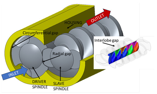
Figure 1.
Main leakage paths and reference twin-screw pump.
The radial gap is defined as the clearance between the tip of one spindle and the shaft of the other spindle, while the circumferential gaps are the clearances between the spindle’s tip and the pump housing. In contrast, the flank gap presents a distinctive challenge due to its intricate 3D geometry, introducing considerable complexity in the establishment of a numerical model. Generically, the ideal displacement of a screw machine is defined as follows:
where A is the wet area of the transversal section and L is the lead, which corresponds to the distance along the spindle’s axis covered by one complete rotation of the screw (360°). It can be calculated as:
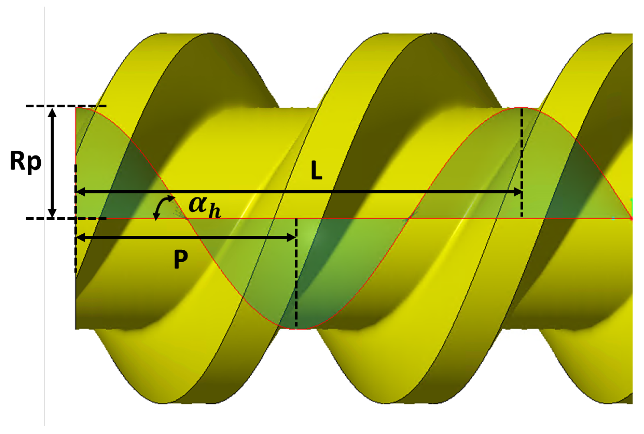
where n is the number of threads and P is the pitch, representing the distance from the crest of one thread to the next one. The helix angle , defined in Equation (3), fixes the final length of the spindle for a given number of pitches, as also visible in Figure 2.

Figure 2.
Relationship between helix angle, pitch, and primitive radius for a two-thread spindle.
In this application case, the driving screw consists of a double-start thread trapped 900° around its corresponding shaft. The driven spindle is a three-start thread resulting in a 2/3 transmission ratio. Figure 1 provides a qualitative representation, and for confidentiality reasons, no additional geometrical parameters are disclosed. The screws are merely entrained within a cylindrical support, delimited by the pump housing. Notably, no bearings are employed to simplify pump manufacturing, a typical requirement in automotive applications. This design choice allows for misalignments of the axis, potentially giving rise to incidental dry friction phenomena between the rotors and casing during pump operation. However, in normal circumstances, the thin film of fluid entrained in the circumferential gap serves to hydrodynamically support the rotating spindles.
2.2. Experimental Setup
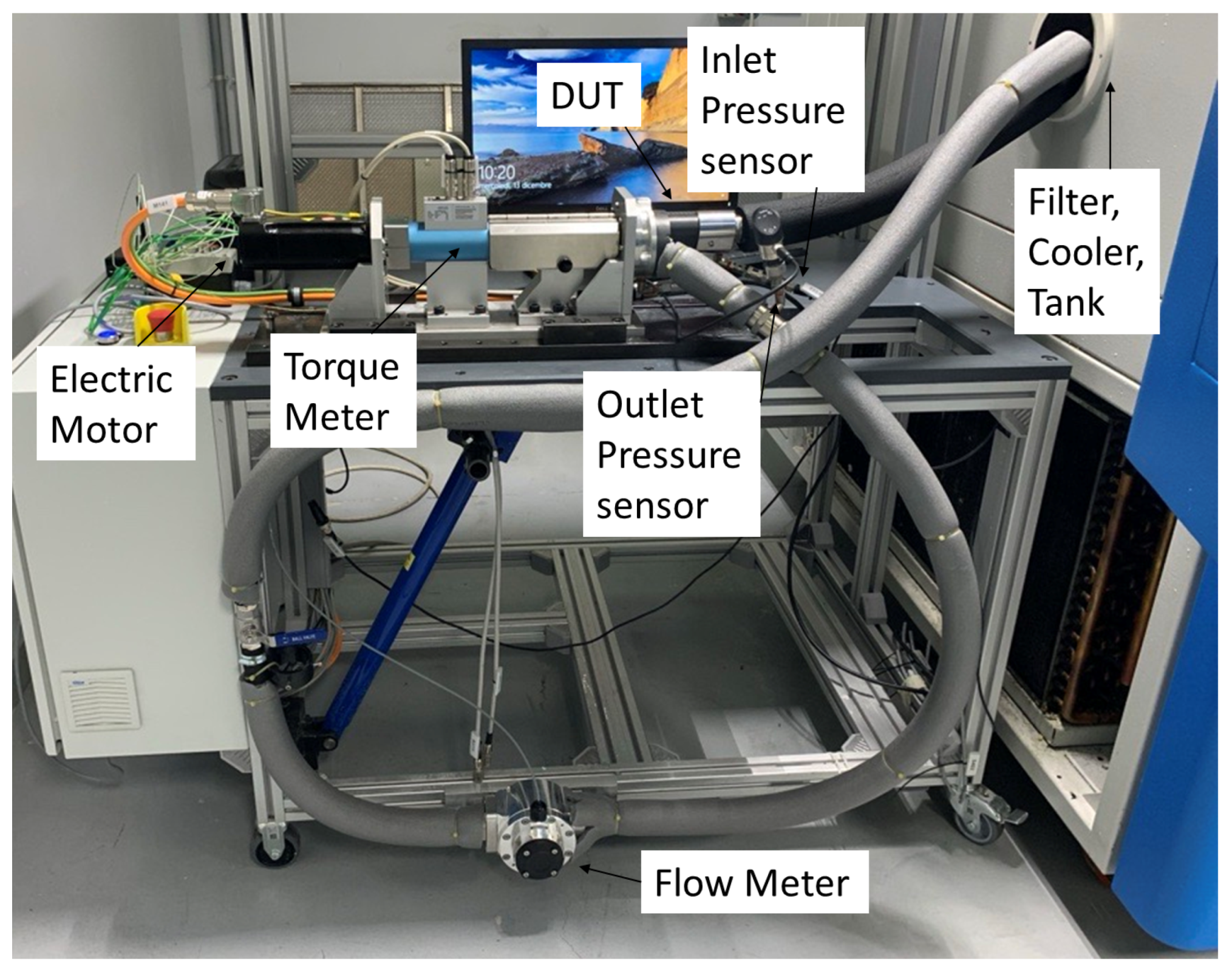
The Experimental setup utilized for the tests is depicted in Figure 3. The test medium consists of a 50:50 mixture of water and glycol (IP Antifreeze Red) at room temperature, featuring a density () of 1070 kg/m3 and a viscosity () of 0.004 Pas. Various operating points are attained by employing a control valve on the discharge side. The rotational speed is systematically controlled and adjusted through a dual-range Torque meter (Kistler Type 4503A). The pressure at the discharge pipe is monitored using an amplified pressure transducer (Unik 5000 pmp), and low-rate measurement in the discharge pipe is carried out using a positive displacement oval gear flow meter (Kobold DON). Additional specifications are provided in Table 1. It is noteworthy that the Experimental test campaign was conducted at the Laboratory of Fluid-o-Tech, an Italian company involved in this research boasting over 70 years of expertise in engineering and manufacturing positive displacement pumps and fluidic systems.
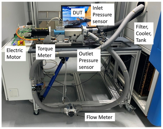
Figure 3.
Hydraulic test rig at Fluid-o-Tech.

Table 1.
Specification of the sensors employed.
3. Simulation Methodology
In this section, the modeling of the reference machine is detailed using three different approaches: unsteady-CFD, steady-CFD, and LP.
3.1. Unsteady-CFD
This subsection involves the mesh generation, mesh convergence study, and setup of turbulence and cavitation models; this has been carried out within one commercial software, SimericsMP+® (v.6.0.4). During normal operation, PDMs induce variation in the pressure within the fluid domain by changing the size and position of the working domain and consequently propelling the fluid. To assess the performances of such machines, numerical modeling of quantities like mass, momentum, and energy is required. The governing equations are a coupled set of time-dependent PDEs solved using an FVM. The commercial software SimericsMP+® was employed for this purpose, with details on the solution scheme available in [28], briefly summarized here. The numerical scheme is grounded in the RANS equations, incorporating a standard k- model to account for turbulence effects. The cavitation phenomena are addressed according to the Singhal model [29], in which the fluid is considered as a mixture of liquid, vapor, and some non-condensable gases. In particular, the Equilibrium Dissolved Gas Model is employed in which the total mass fraction of the non-condensable gas dissolved in the liquid is equivalent to the equilibrium value. Simulations were conducted with a reference pressure of 1.01 bar at the pump inlet, while the pump outlet pressure varied up to . By adjusting the pressure difference between the inlet and outlet, the desired flow rate was attained. The rotational speed of the driver rotor ranged from up to . Stagnation inlet and pressure outlet conditions were applied to the respective inlet and outlet boundaries. Initial conditions included a starting pressure of 1.01 bar, an initial velocity of 0 m/s, a turbulence intensity of 1%, and a turbulence viscosity ratio of 10.
Grid Generation
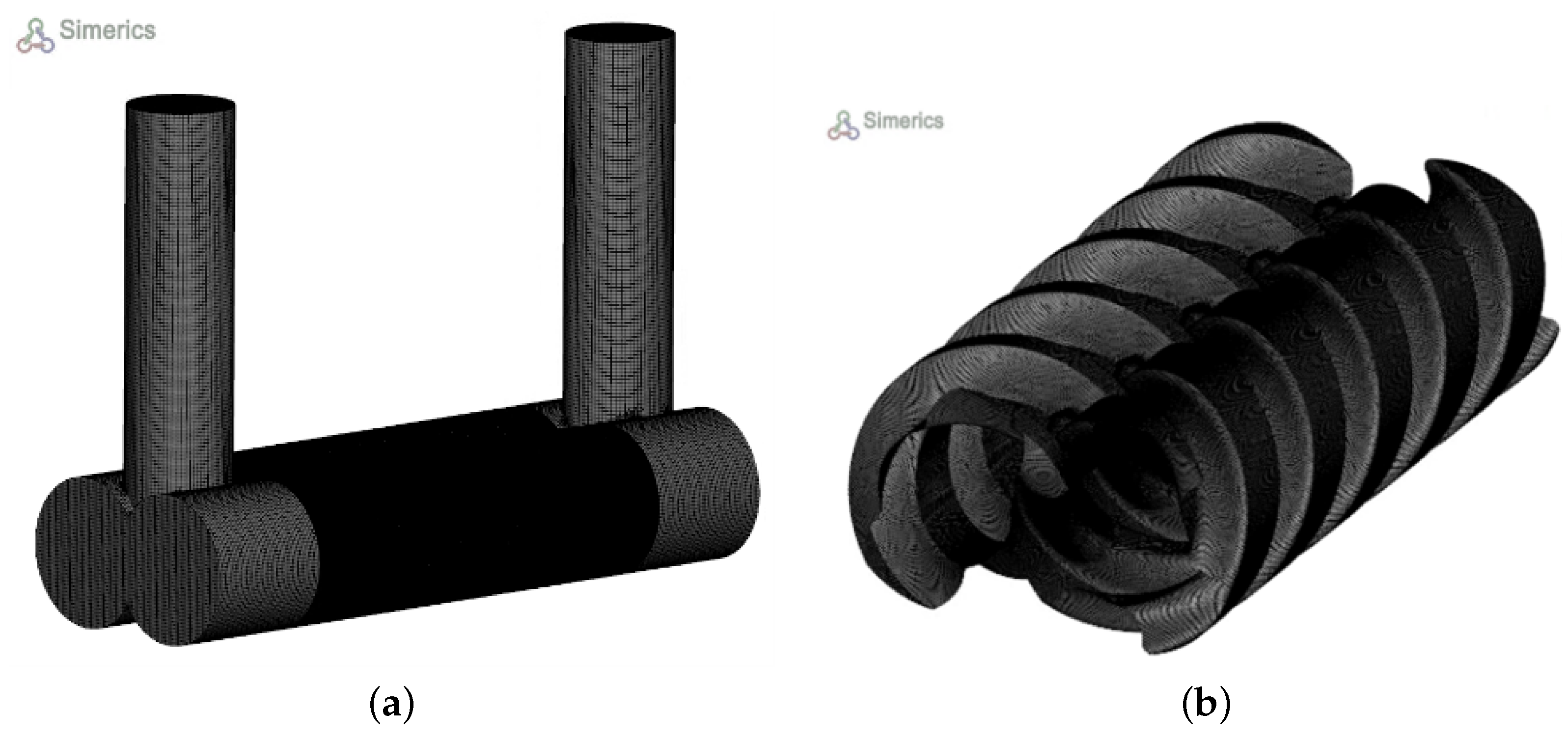
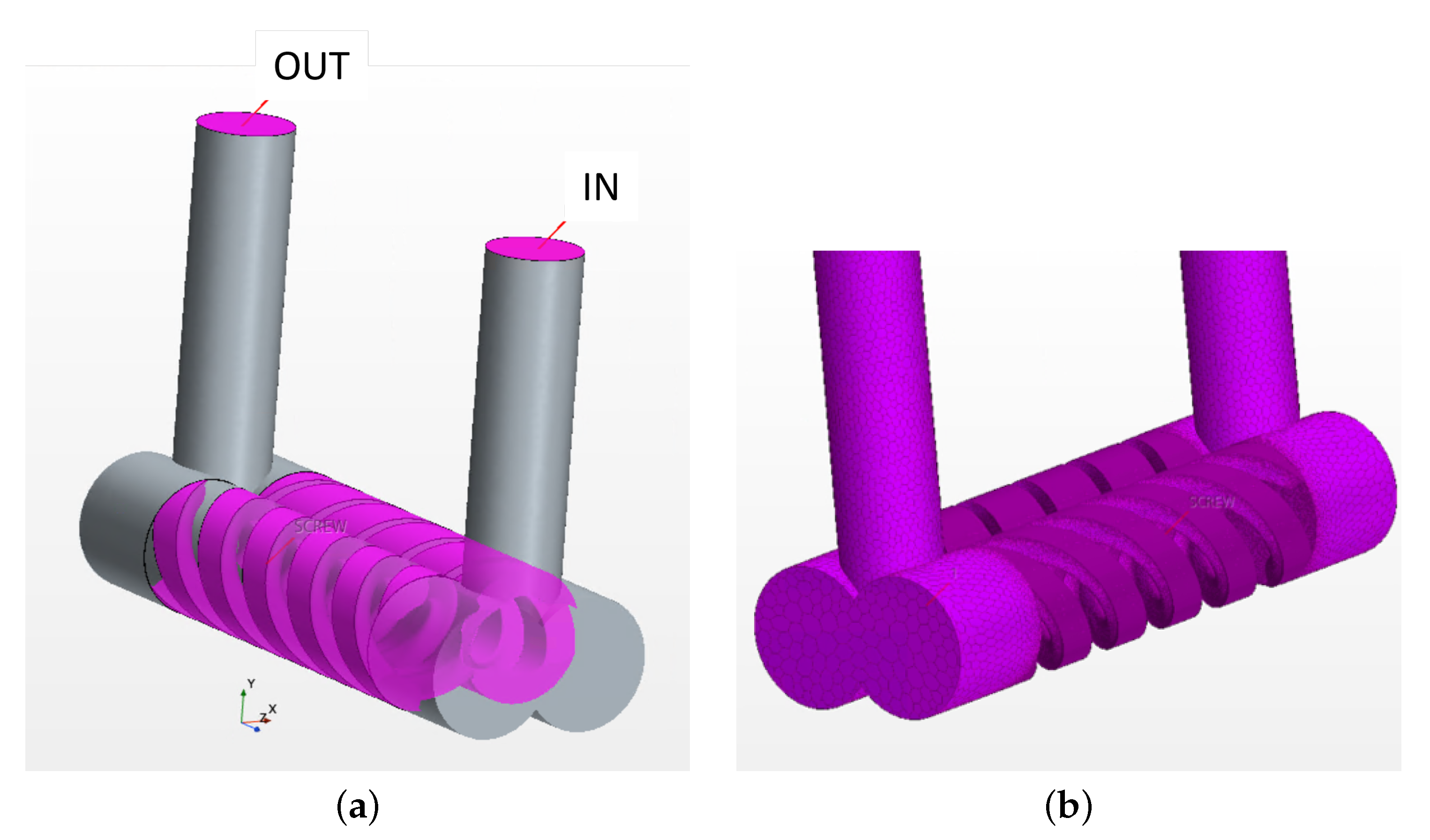
Mesh generation involves discretizing the working domain into control volumes to establish local fluid properties’ solutions. In this study, the SimericsMP+® grid generator facilitates the discretization of the computational domain. The VOF domain, depicted in Figure 4a, was derived from the 3D CAD drawing using the Creo® software (v.7).
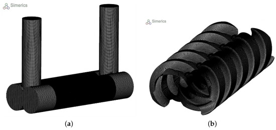
Figure 4.
Volume of fluid representative of the reference machine: (a) Entire VOF meshed using Simerics MP+. (b) Detail on the mesh of the spindles.
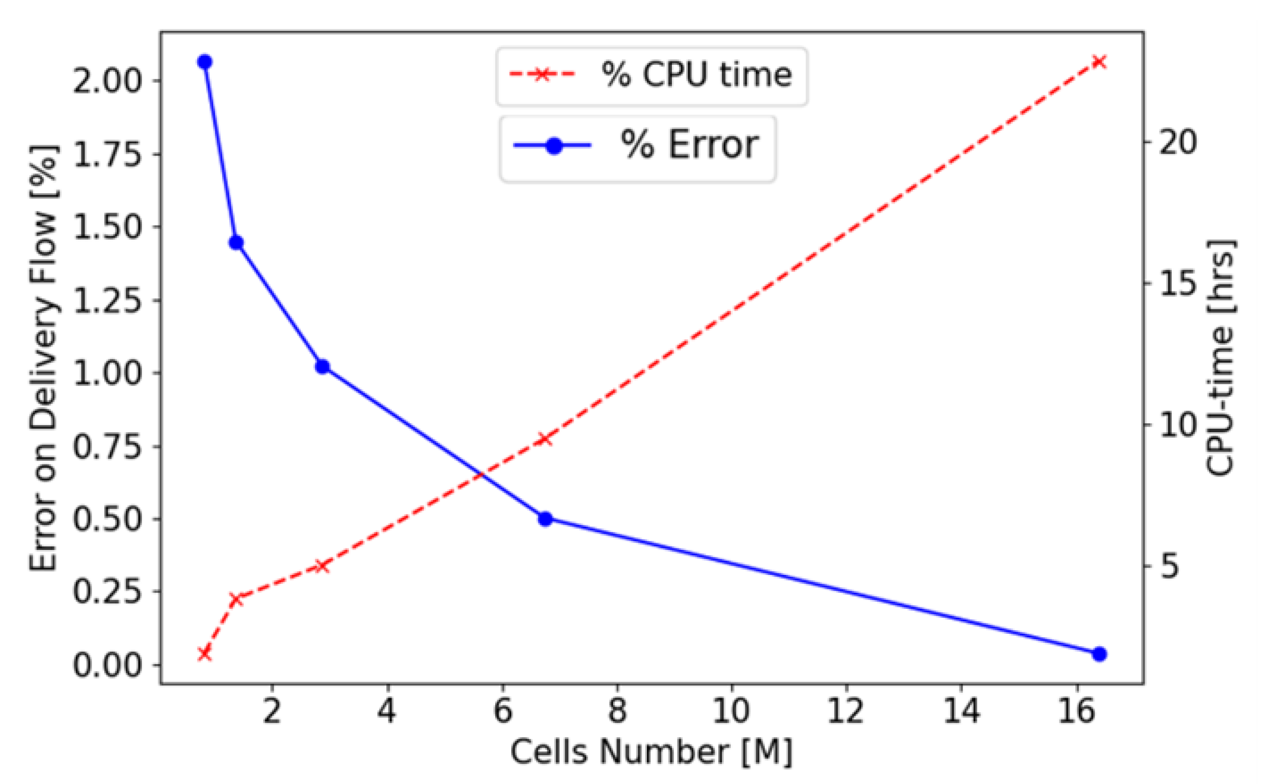
This domain was subdivided into sub-volumes, subsequently interfaced in SimericsMP+® through an implicit interface known as the mismatched grid interface. The VOF was then imported into the CFD code in STL format and meshed with appropriate grid sizes. For the static mesh of the inlet and outlet ports, an unstructured body-fitted binary tree approach was employed, utilizing SimericsMP+®’s general grid generator. Meanwhile, for the spindles, whose working domain changes and deforms over time, the new General Gear rotor template mesher for spindle machines was adopted, as illustrated in Figure 4b. A mesh sensitivity analysis was conducted to ensure the independence of the outlet volumetric flow rate from the cell size, as depicted in Figure 5. The VOF comprises approximately 2.87 million cells, with specific settings for the rotor mesher in the structured spindle volumes, including 120 cells in the circumferential direction, 8 in the radial direction, and 600 in the axial direction. Although models with finer meshes were explored, the results did not justify the increased computational time.
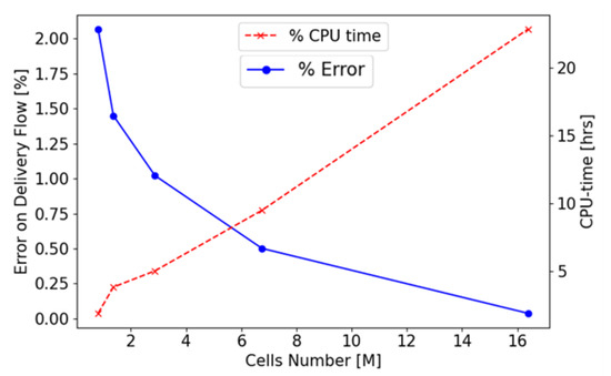
Figure 5.
Mesh sensitivity.
3.2. Steady-State CFD
In this section is presented the setup for the steady-state CFD simulation of the reference machine using the commercial software Siemens Star-CCM+ (v.2206). Figure 6a illustrates the imported geometry, highlighting the rotor fluid domain, static ports, and input and output boundaries. Notably, the negative volume of the spindles’ geometry—the fluid volume—has been directly extracted from the CAD and imported into the software.

Figure 6.
(a) Description of the VOF. Focus on the fluid domain pertinent to the spindles and boundaries. (b) Comprehensive mesh of spindles and ports.
In addition to the ports and spindles’ volume, circumferential gaps have been generated to replicate the fluid between the external diameter of the spindles and the internal diameter of the housing. These three parts have been linked to a region with identical physical properties. The connection between these parts is facilitated by creating interfaces, which can be categorized into three types: the interface between the spindles’ outer surface and gap, the spindles’ top and bottom surface to the ports, and the gaps’ top and bottom area to the ports, as shown in Figure 7. As depicted in Figure 6b, a polyhedral mesh has been selected for the spindles and ports domains. By imposing a mesh target size near the interfaces, the mesher automatically refines towards the most-critical areas. For the spindles, a prism layer mesher was employed along the contours to control the number of layers and cells near leakage zones. A prism layer mesh type was used to mesh the thin gap part, extending along the length of the spindles according to their curvature. Seven layers were considered, resulting in almost 4.5 million cells for the VOF domain, as shown in the zoom-in Figure 7. It is important to note that a k- turbulence model has been incorporated, as described in Section 3.1, while no cavitation model was considered. Simulations were executed for various outlet pressures until the stopping criteria of residual convergence or reaching the maximum number of iterations, set at 100,000, were met.
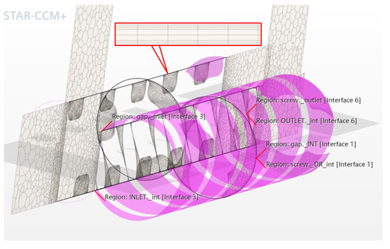
Figure 7.
Interface between the three main parts: spindles, ports, and circumferential gaps.
3.3. LP
Taking inspiration from the workflow outlined by Vacca [30], the authors propose a novel methodology, as depicted in Figure 8. Notably, this approach has never been previously applied to screw pumps and is well suited for modular development, allowing the seamless integration of additional subroutines to predict various aspects, as successfully demonstrated by Ransegnola [17].

Figure 8.
Structure of the proposed methodology.
The primary objective of this methodology is to predict the pump’s performance starting from its geometry. The Geometrical Module elaborated in Section 3.3.1, plays a pivotal role in this process. Here, a new geometry can be generated using the Screw Generator or read from an existing CAD using the Surface Tool, following the structure described in Figure 8.
Subsequently, the Geometrical Module conveys information about control volumes and other features in the form of a text file to the Fluid Dynamics Module, detailed in Section 3.3.2. The Fluid Dynamics Module is the core of the Simulation Module, where the pressure inside the TSV is evaluated. The information elucidated by the Geometrical Module also serves as the input for the Force Module. The Force Module, detailed in Section 3.3.3, Analytically predicts the Real Torque at the pump’s shaft by considering geometrical parameters, fluid properties, and the materials from which the spindles, housing, and other main components are made.
3.3.1. Geometrical Module
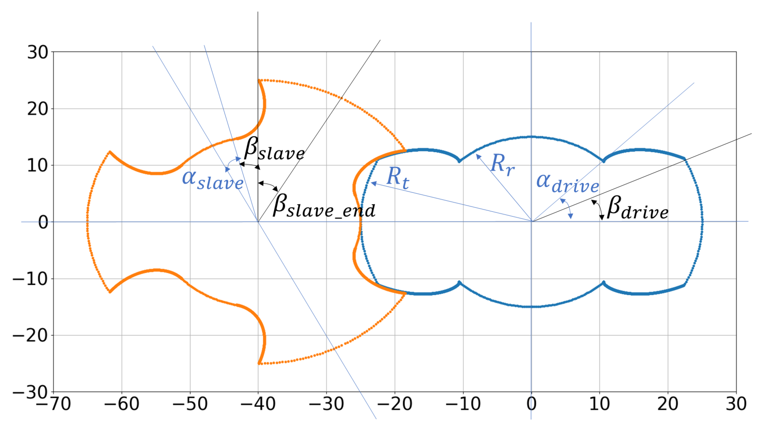
The Geometrical Module functions as a vital pre-processor for all Modules within the simulation Tool, focusing on evaluating key features essential for analyzing the Fluid Dynamics properties of a hydraulic machine, including the DC volume and porting areas. Users are presented with two options within the Geometrical Module: generating a new geometry through the Screw Generator or importing an existing one as a .TXT or .DXF. Upon obtaining the profiles, the Surface Tool operates, generating the , critical for the Fluid Dynamics Module. To enhance clarity regarding the Surface Tool’s functionality, the working principle of the Screw Generator is introduced first. Specifically, a type-D geometry, as described by Yan [31], is illustrated. In the end, it outputs a 2D list of coordinates for each spindle, as depicted in Figure 9. For type-D spindles, following the inputs and their relationships detailed in Table 2, the rotors are systematically constructed.
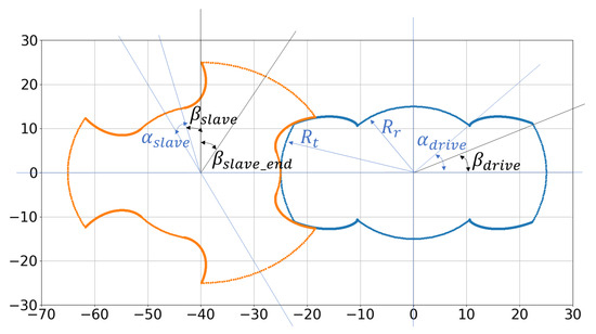
Figure 9.
Type-D profiles, generated using Screw Generator. Angles of reference.
Table 2.
Input parameters and their relationship for the Screw Generator.
First, the generation of the main spindle is introduced: due to its symmetry, the equations for the generation of 1/4 of the geometry are reported. Equation (4) describes the root circle for the main spindle, and it is valid for .
The cycloidal arc is described in Equation (5). It is parametrically defined using an angular variable (). The loop iterates until the condition is satisfied, ensuring that the points lie within a specified circle. The exit coordinates identifies . Evidently, Equation (5) is valid for (90 −).
Equation (6) describes the external arch that completes the main spindle, valid for .
The slave spindle is generated with the same Geometric instances of the circle arcs and the cycloid arc. Only 1/6 was generated considering its symmetry. Please note that the slave spindle shown in Figure 9 has been rotated to avoid any overlap. Equation (7) describes the internal arc generation, which is valid for .
where:
To generate the coordinate points (, ) representing the cycloidal curve of the slave spindle, the curve is parametrically defined using an angular variable () and involves what is specified in Equation (9). The loop iterates until the condition is satisfied, ensuring that the points lie within a specified circle, identified by the external diameter of the rotors. The exit point individuates .
In the end, Equation (10) describes the external arch that completes the slave spindle.
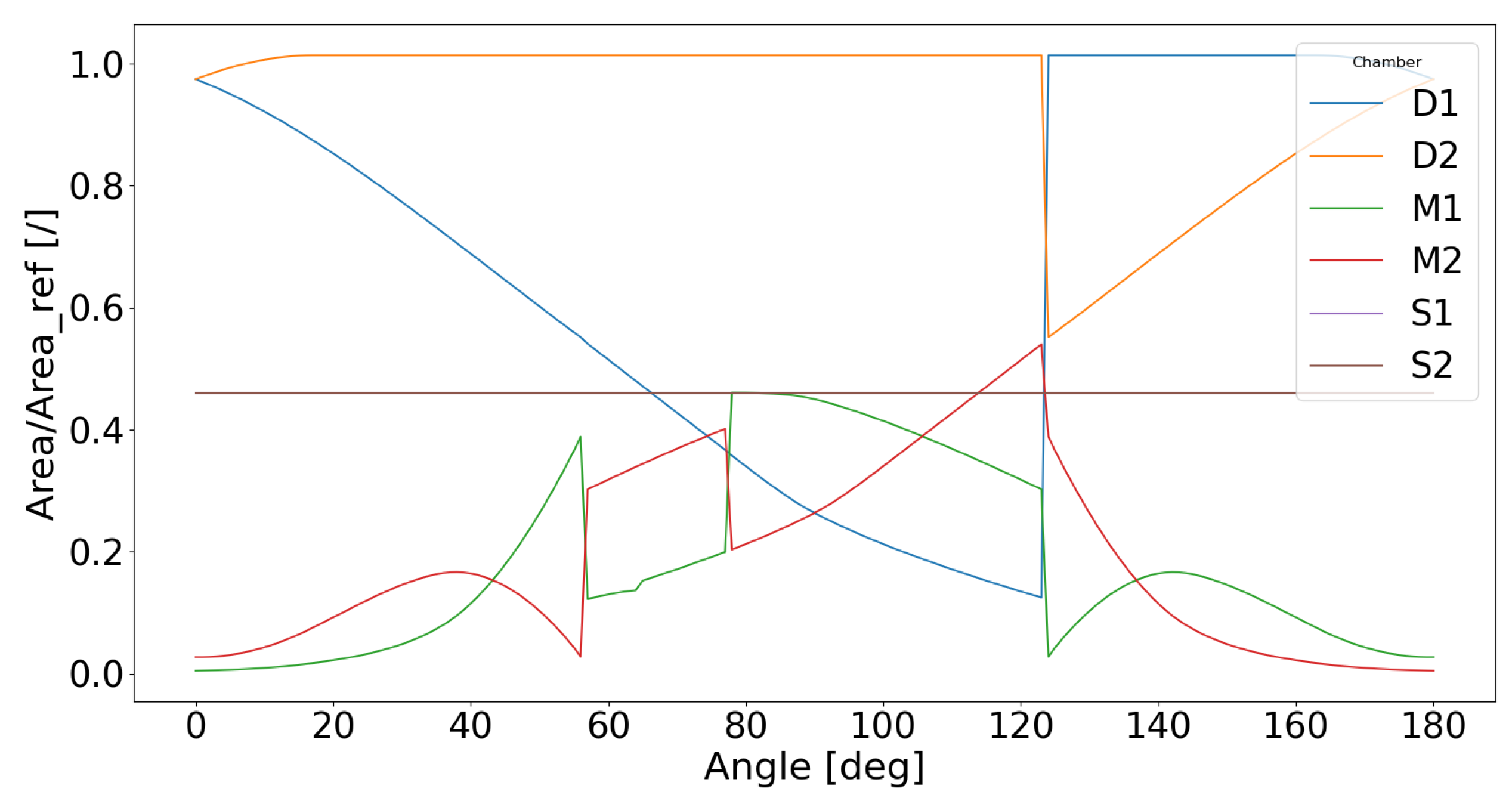
Once the profiles of the spindles are available, the Surface Tool comes into play. In Figure 10, six distinct areas, referred to as chambers, are defined by the Surface Tool, providing their values for every rotational angle of the drive spindle. In addition to the previously introduced and values, Figure 10 illustrates segment lines identifying the characteristic angles crucial for describing the pump housing. These angles play a pivotal role in defining the chambers during rotation. Considering the counterclockwise direction of rotation of the main spindle, Figure 10 offers a qualitative depiction of the evolution of each chamber. For a more-quantitative understanding of the output from the Surface Tool, Figure 11 is presented. It is evident that M1 and M2 consistently define the volume of fluid entrapped between the two spindles, open to the meshing zone. On the other hand, S1 and S2 represent the volume of fluid entrapped between two starts of the slave spindle within the casing. D1 and D2 predominantly delineate the volume of fluid in contact with the main spindle.
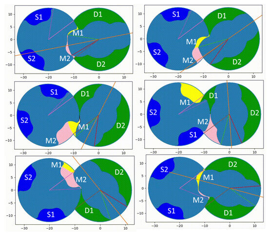
Figure 10.
Qualitative description of Surface Tool.
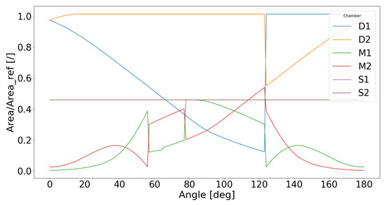
Figure 11.
Evolution of chambers as calculated by the Surface Tool.
3.3.2. Fluid Dynamics Module
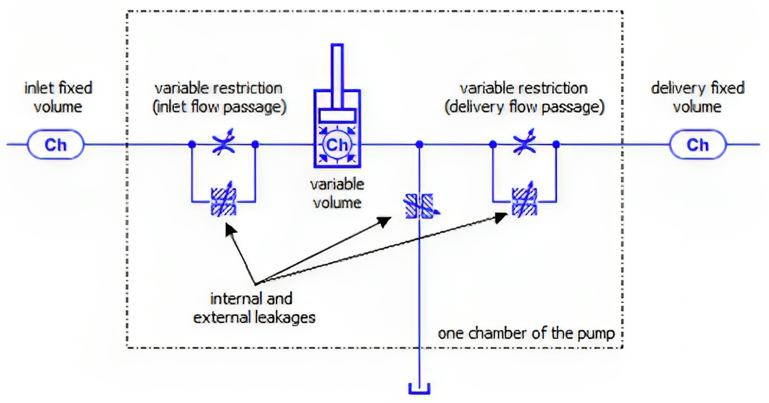
The Fluid Dynamics Module processes the inputs from the Surface Tool to calculate the flow-pressure pump characteristic curve. Within each chamber, fundamental properties like density, pressure, temperature, and viscosity remain constant, forming the basis of a lumped-parameter model. This choice allows for fast computations and easy integration with potential sub-Modules. In this project, Simcenter Amesim (v2021.2), a commercial software, was employed to implement the LP model. As outlined in [32], a volumetric pump utilizing an LP approach is modeled as depicted in Figure 12.
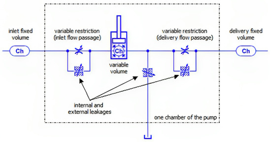
Figure 12.
Generic LP modeling of a volumetric pump using Simcenter Amesim.
The pressure build-up equation is a differential equation solving for the conservation of mass in a lumped fluid domain. Further details regarding the derivation and assumptions are elaborated in the book by Vacca and Franzoni [33]. The formulation assumes an isothermal process, but can be extended for non-isothermal cases. The equation is as follows:
where and establish a one-to-one relation between density, bulk modulus, and pressure in an isothermal case with temperature T. To accommodate air and vapor, the formulation assumes an equivalent density and bulk modulus, capturing the effective compressibility of the liquid–gas solution. In this approach, properties like effective bulk modulus, viscosity, and density become functions of pressure and temperature, directly integrating aeration and vaporous cavitation phenomena into the fluid property relation with pressure and temperature. For instance, in this assumption, a specific pressure and temperature correspond to a distinct amount of gas mass fraction in the fluid domain, denoted as . This assumption is commonly referred to as a static assumption, as discussed by Mistry [34]. Figure 13 illustrates a potential implementation of the screw pump using an LP approach, emphasizing its validity within a specific angular range of the driving spindle.
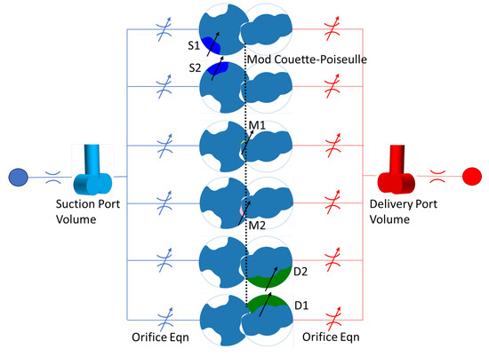
Figure 13.
Representation of TSVs and internal connection. Valid for a certain angular range.
Unlike the implementations of other pumps, such as gerotor pumps, as done by Pellegri [35], vane pumps, as done by Mistry [36], the spur EGM, as shown by Marinaro [37], or the helical EGM, as discussed by Mazzei [38], where each TSV maintains a consistent connection, spindle machines introduce complexities due to the intricate behavior in the meshing zone. The evolution of chambers, as depicted in Figure 10, reveals that each TSV undergoes a dynamic connection with different chambers throughout its rotation, making the conventional treatment challenging. To address these challenges, the authors propose a simplified approach depicted in Figure 14.
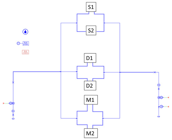
Figure 14.
Stationary model of a spindle pump in Simcenter Amesim.
This model ignores the characteristic helical shape of the fluid volume and approximates each chamber as developing straight along the pitch. As illustrated in Figure 15b, the connections for M1 and M2 are modeled using the orifice equation, while a modified Couette–Poiseuille approach, as proposed by Rituraj [39], is applied for the others. This simplified representation facilitates the modeling process and captures essential aspects of the screw pump’s behavior.
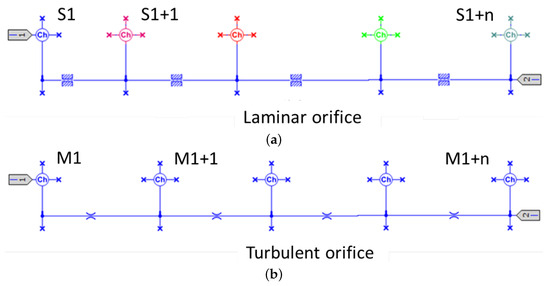
Figure 15.
(a) Actual implementation of modeling for S1, S2, D1, and D2 chambers. (b) Actual implementation of modeling for M1 and M2 chambers.
Regarding chambers chambers and , the fluxes have been modeled as a turbulent non-circular orifice. The mass flux into volume is given by:
where:
- is the flow coefficient [40].
- A is the cross-sectional area (mm2) of the orifice.
- is the pressure difference (bar) between the chambers.
- is the average working fluid density (kg/m3) between two chambers.
To account for different flow regimes and orifice geometries, is described as:
where:
- is the maximum flow coefficient defined by the user.
- is the flow number.
- is the critical flow number [40].
Therefore, the value of depends on the flow number as follows:
where:
- = is the orifice’s hydraulic diameter (mm).
- is the kinematic viscosity evaluated at the average pressure (mm2/s).
The hydraulic diameter of the non-circular orifice has been calculated as a function of the orifice area and its wet perimeter.
Considering the leakage flow at the tips of the spindles, it can be treated as leakage flow through thin sections [41]. This leakage connection comprises pressure-driven flow (Poiseuille) and relative-body-motion-driven flow (Couette). Couette flow results from the relative motion of two surfaces surrounding the liquid. The relation for this flow can be calculated for a specific geometry, but the fundamental equation between two flat plates is:
Depending on the geometry considered, the Poiseuille equation can be formulated for curved surfaces and flat surfaces. The Poiseuille equation for a flat surface is:
For curved surfaces, the Poiseuille equation is given by:
here, represents only a pressure-driven flow through a section defined by two curved geometries with an equivalent radius of curvature of , a pressure difference of , and a gap height of h, as introduced by Rituraj [39].
3.3.3. Forces Module
In this section, the Analytical Force Module, which allows for the prediction of the Real Torque andeach Force’s contribution, is described. The Real Torque () is given by:
where is relative to the Torque losses relative to the driver spindle, while is relative to the Torque losses due to the driven spindle. represents the losses due to the contact between the two spindles, which is not ideal. represents the transmission ratio, due to the fact that the spindles have a different number of stars. As defined by [41], the ideal Torque is given by:
As illustrated by Ivantysynova [41], Torque losses in hydraulic machines can be subdivided into the following components: losses dependent quadratically on speed, losses dependent proportionally on speed, losses dependent proportionally on pressure, and losses independent on the operational parameters. The Torque losses relative to the spindle x can be generically written as:
The first class () expresses the Torque losses due to velocity effects due to frictional effects in the turbulent region. The second term () represents the losses to overcome due to viscous friction between the sliding surfaces of the displacement machine. The third term () represents the Torque losses dependent on pressure due to contact between surfaces. In particular, two terms have to be considered. The first term of Equation (21) () represents the loss due to the spindle–housing contact. The second term () represents the Torque loss due to spindle–axial stopper contact. Axial stoppers are needed to counterbalance the axial load on the spindles due to the pressure difference between the inlet and outlet side and are shown in Figure 16.
is independent of the operational parameters and can be influenced by manufacturing tolerances, initial stress on the seals, and other preloaded parts. In this specific case, it represents a constant contribution due to the presence of mechanical sealing on the pump shaft.

Figure 16.
Visual representation of: axial stoppers (i.e., pins) for counterbalancing the axial load, wet transversal areas (), and main spindle’s threads’ wet area ().
Expanding each of the terms, Torque losses due to velocity effects can be written as:
where (/) represents the coefficient of friction for viscous and velocity terms. Its value depends on the materials and lubricants [42]. () represents the fluid density. represents the transmission factor. It is equal to 1 for the driver spindle and equal to 2/3 for the driven spindle (because, in this specific application case, has two starts and has three). v (m/s) represents the velocity and can be written as:
where n (rev/min) is the rotational speed. () represents the wet area relative to . (m) is the external radius of the spindles.
The wet area () is shown in Figure 16 and can be calculated as proposed by Di Giovine [43] or measured using the CAD.
Torque losses due to viscous effects relative to can be written as:
where (Pa·s) represents the dynamic viscosity and h (m) represents the radial circumferential gap, introduced in Figure 1.
The Torque due to friction between and the pump housing can be written as:
where (/) represents the friction coefficient due to the contact between the bodies in contact, and its dependency on the materials and operating conditions is discussed in [44]. (m) represents the primitive diameter relative to . represents the radial Force acting on the spindle due to the linear evolution of pressure along the spindle’s axis, discussed in detail in Section 4.1. represents the radial decomposition of the ideal Force acting on the pressure line. can be calculated as [45]:
(/) represents the number of pitches for the given spindle. L (m) represents the total length of the spindle. (/) represents the number of starts for the given spindle. (N) represents the radial contribution of the Force, i.e., the tangential Force along the primitive circle, calculated as:
The ± sign is used because this contribution can either add or relieve the load whether the helix is clockwise or counterclockwise.
Ultimately, the Torque losses due to the contact between spindles and the axial stopper can be expressed as:
(m) represents the external radius of the stopper in contact with the spindle; (2/3) is the equivalent contact area according to Hertzian theory [46]; (N) is the Force contribution due to the resultant axial pressure, equal to:
where is the wet transversal area of , highlighted in Figure 16.
(N) represents the axial decomposition due to the helix angle () of the ideal Force acting on the pressure line and can be calculated as:
In the next section, the methodology described in Section 3 will be validated and compared against experiments across a wide range of operating conditions.
4. Results and Validation
This section presents results from the unsteady-CFD, steady-CFD, and LP models, offering insights into each numerical approach and carrying out a comparative analysis.
4.1. Flow-Pressure Characteristic Curve
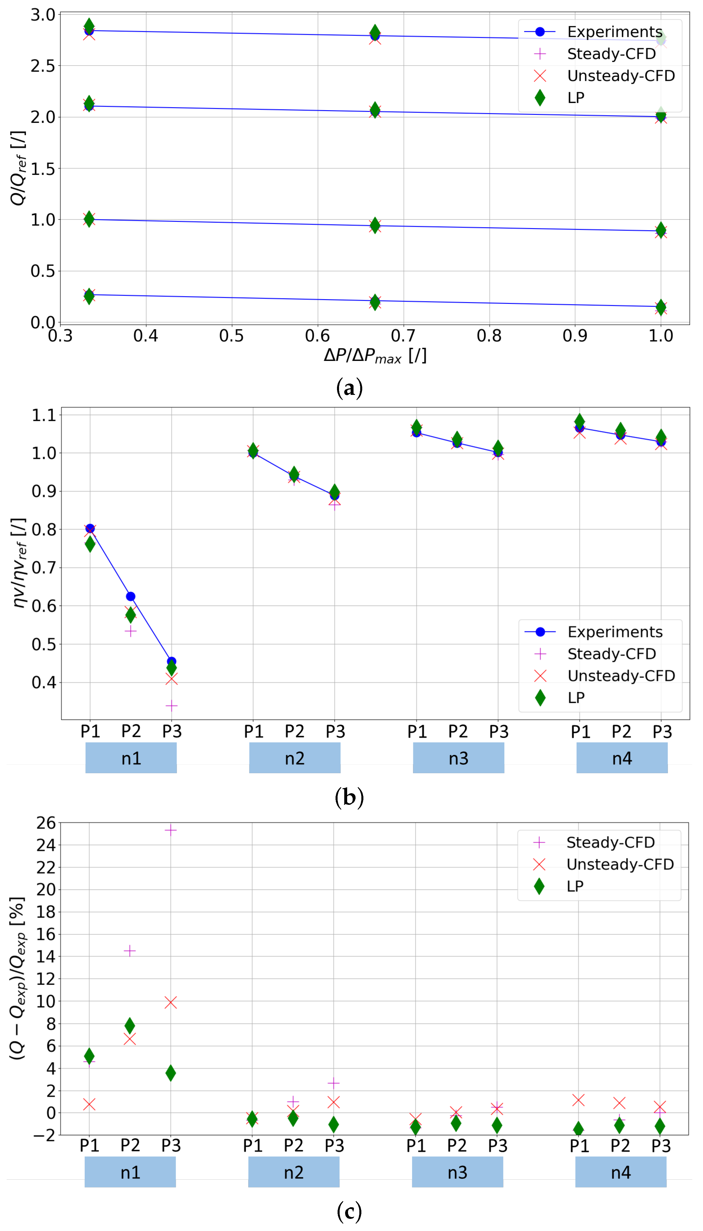
At first, steady-state characteristics are presented. Figure 17a illustrates the alignment of the flow-pressure characteristic curves predicted by all models with the measured flow (blue lines).
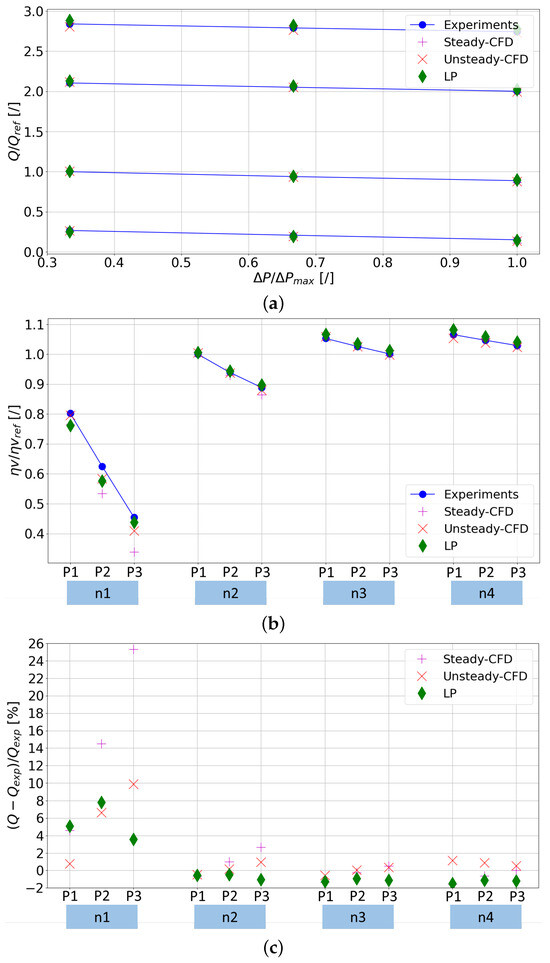
Figure 17.
(a) Flow-pressure curves. (b) Volumetric efficiency. (c) Percentual error with respect to Experimental flow rate.
The fact that the flow is almost constant over the pressure is a characteristic asset of volumetric machines, and in particular, it highlights the good volumetric behavior of the specific machine. Figure 17b details the volumetric efficiency across different motor speeds and pressure drops. The discernible shift in slope from low to high speeds signifies that leakages primarily exhibit pressure-driven characteristics, showing minimal influence from motor speed. To assess the predictive accuracy, Figure 17c depicts the percentage error relative to the measured flow rate for each (n, P) combination. A comprehensive summary of the average and standard deviation values is outlined in Table 3.
Table 3.
Overview of models’ performances in experiments.
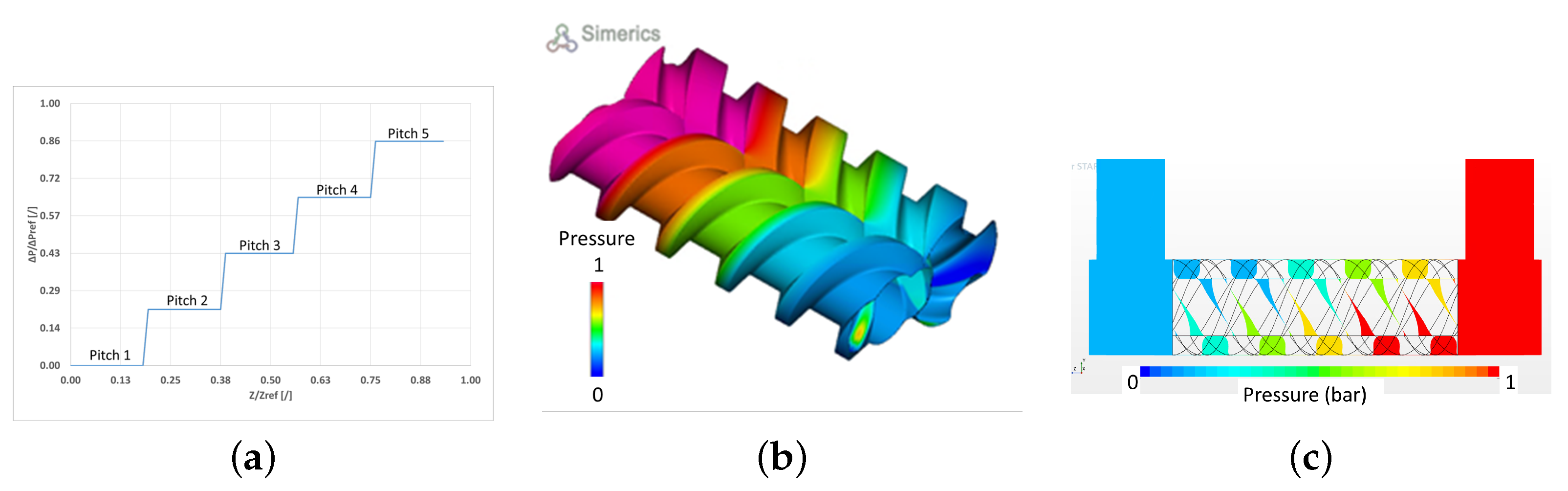
By examining the results shown in Figure 17 and reported in Table 3, the LP model emerges as the most-accurate across the different scenarios. Despite the overall success, a noteworthy challenge arises at the low-speed high-pressure corner point. Here, the absence of bushings allows the spindles to move freely within the pump housing, with their radial position contingent on both pressure and speed. In fact, pressure and speed influence the hydrostatic and hydrodynamic contributions to the fluid film between the spindles’ tip and housing. At the low-speed high-pressure corner point, the hydrodynamic contribution diminishes, leading to spindle–casing contact due to the radial component of the Force derived from the pressure difference. This specific behavior, attributed to the unique characteristics of the reference machine, is not fully captured by existing models. In CFD approaches, the radial position of the spindles is fixed, and the LP model does not account for spindle motion at this moment. The pressure distribution, illustrated in Figure 18, underscores two key observations. Firstly, the mean pressure gradually rises along the axial direction from the inlet to the outlet port, a phenomenon accurately represented by all three approaches. Secondly, due to the helical shape of the spindle, the lower portion of each chamber advances axially, reaching higher pressure levels sooner. Consequently, the spindle body experiences a resultant Force that may induce shaft deformation and radial movement of the spindles. Importantly, the current simulations assume a perfectly rigid spindle, disregarding structural deformation. To address radial spindle movement instead, a pragmatic approach involves rigidly moving the spindles toward the lower-pressure side, maintaining a minimum gap of 5, μm, as previously detailed by the authors [47].

Figure 18.
Pressure distribution along spindles’ axis: (a) LP; (b) unsteady-CFD; (c) steady-CFD.
4.2. Torque Prediction
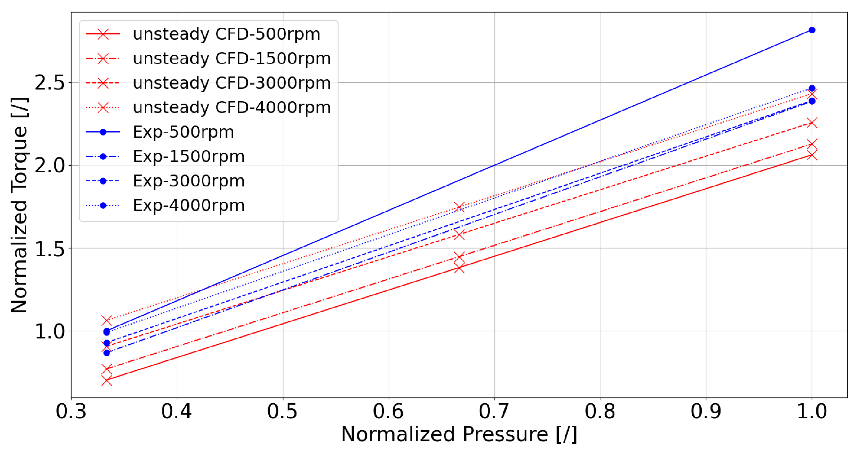
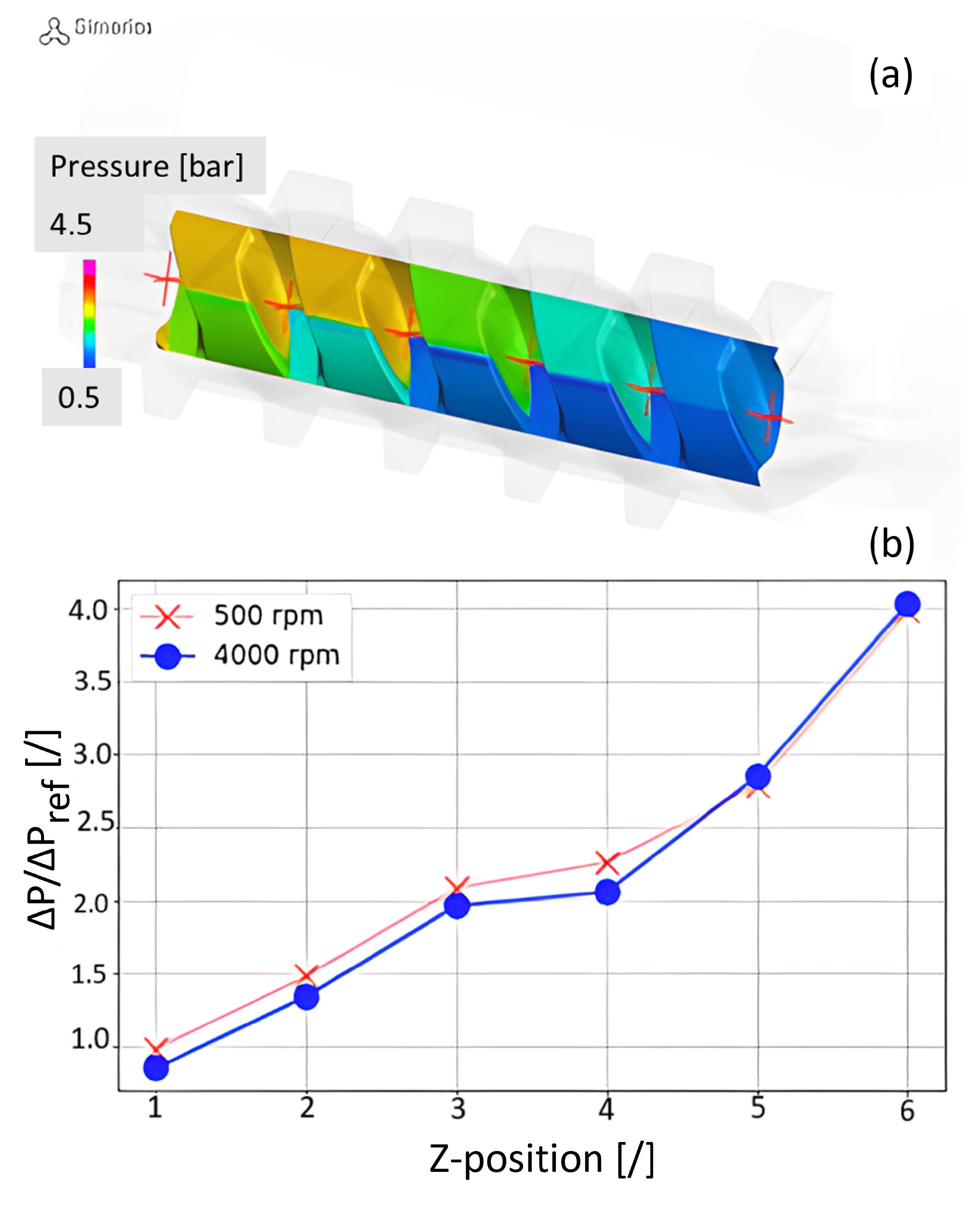
Concerning Torque prediction, steady-CFD cannot be used. Figure 19 shows the comparison between the unsteady-CFD numerical results and Experimental Torque at two different P and over four different motor speeds. Looking at the Experimental results, it can be said that Torque is almost independent of speed and linear with pressure, as one would like it to be. Excluding the results at 500 rev/min, the maximum error is 11.2%, with an average error of 4% and a standard deviation of 0.06. Considering that the Torque predicted by CFD is mainly due to pressure and viscous effects, the limited difference underscores the marginal contribution of the frictional effects (spindle-to-spindle and spindles-to-casing). Concerning the numerical results, while at 1500 and 3000 rev/min, the Torque predicted from CFD tends to underestimate the Real Torque, as expected, at 4000 rev/min, the trend is the opposite. This can be explained by looking at Figure 20: six probing points were placed along the spindle’s axis direction; the pressure of each of those points has been plotted.
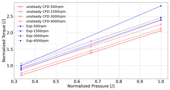
Figure 19.
Normalized Torque versus pressure, unsteady-CFD and Experimental results.
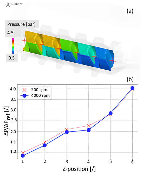
Figure 20.
Torque analysis: (a) six probing points along spindles’ axis in the CFD model; (b) local pressure plotted for each point.
It is evident that the higher the speed, the higher the pump’s suction capability is, resulting in a lower pressure at the spindles’ inlet side, eventually meaning that the P the spindles have to overcome at 4000 rev/min is bigger than at 500 rev/min. At 500 rev/min, the higher Experimental Torque is due to an incompletely developed lubrication regime, as expounded in Section 4.1.
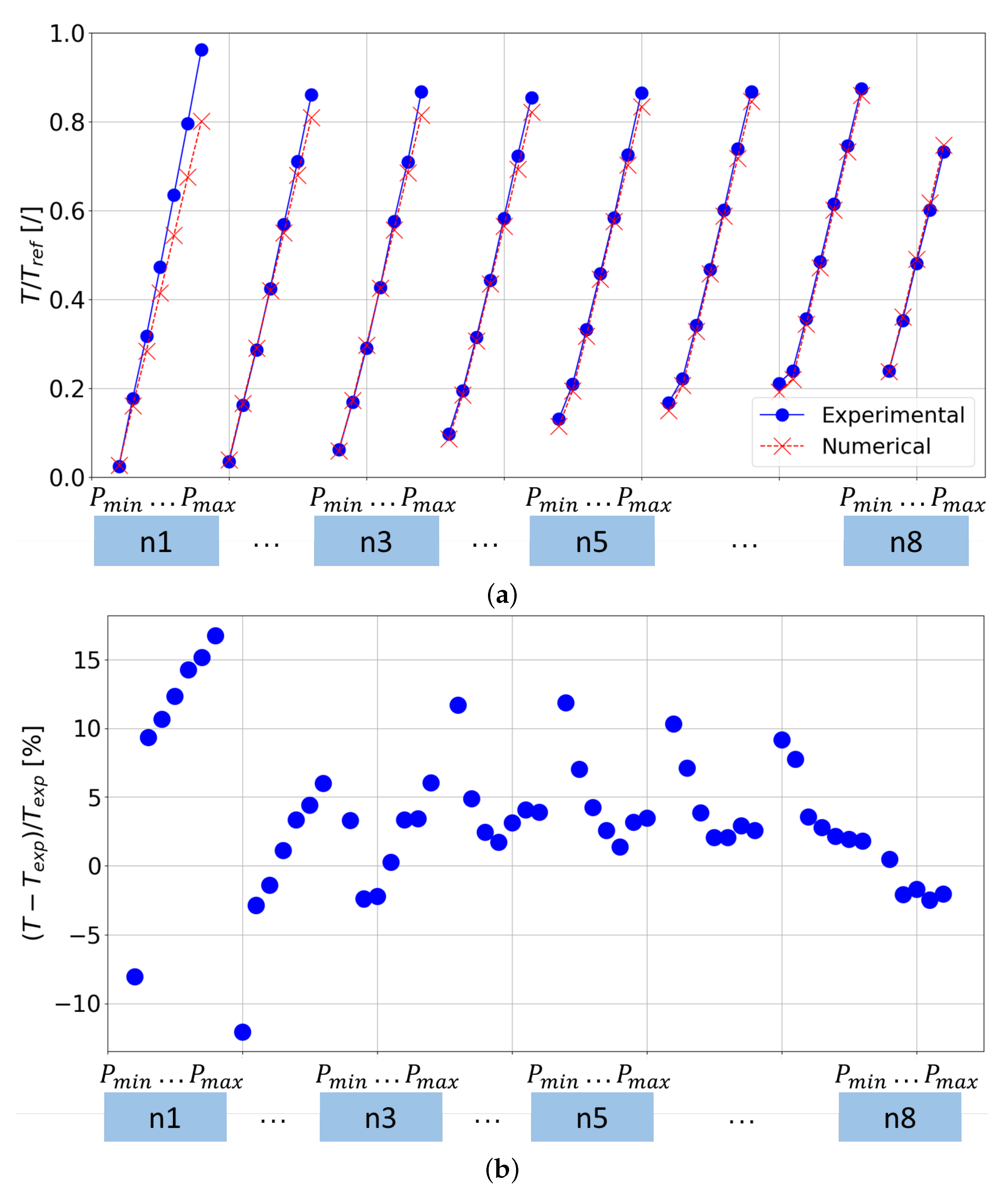
Alternatively, the Analytical approach discussed in Section 3.3.3 provides good accuracy in predicting the Real Torque and allows examining each factor contributing to it. Figure 21a presents a punctual comparison between Experimental and numerical Torque output by the Force Module over a wide range of rotational speed and downstream pressure. Figure 21b reports the percentual error between the Analytical and measured Torque for each point of Figure 21a. A good agreement between the Experimental and Analytical Torque can be appreciated over the whole range of operation. The average error is 3.6%, with a maximum error equal to 16.7%. It can be noted that the highest errors coincided with the lowest speed, as for the CFD model, due to dry friction phenomena.
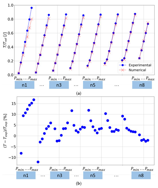
Figure 21.
(a) Adimensional Experimental and Analytical Torque; (b) Percentual error between Analytical and Numerical Torque.
Ultimately, the Analytical model can assist in assessing the contribution of all sources of losses to the Real Torque. Figure 22 illustrates this across various operating conditions. It is noteworthy that the ideal Torque exhibited the most-significant contribution, as expected. The primary sources of losses arose from the contact between the spindles and housing, along with the losses attributed to the velocity effects.
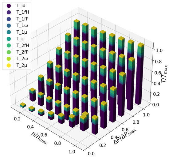
Figure 22.
Torque losses’ distribution across several operating conditions.
4.3. Cavitation
This section delves into considerations regarding cavitation phenomena, leveraging the insights provided by unsteady-CFD simulations. This approach enables the monitoring of the time-dependent evolution of the velocity and pressure distributions, crucial factors in identifying potential cavitation occurrences. Cavitation risks manifest at distinct locations: the spindle leading edge, radial gaps, and flank gaps, as detailed in [26]. The pressure differences across threads in flank gaps, illustrated in Figure 20, result in locally elevated velocities and diminished static pressure. Meanwhile, circumferential gaps experience heightened velocities due to rapid rotation, inducing increased pressure losses in the chamber’s lower section. This leads to a reduction in total pressure and a simultaneous elevation of dynamic pressure, resulting in lower static pressure at the chamber’s bottom. Figure 23 punctually delineates regions where free gas is present, notably at both radial and circumferential gaps, primarily on the lower clearance side. As expected, going from lower (Figure 23a) to higher (Figure 23b) speed, the severity of cavitation increased drastically.
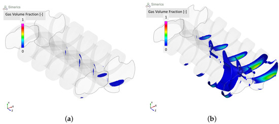
Figure 23.
Isosurface of gas volume fraction: (a) low speed; (b) high speed.
4.4. Fluid Dynamics Optimization of the Porting
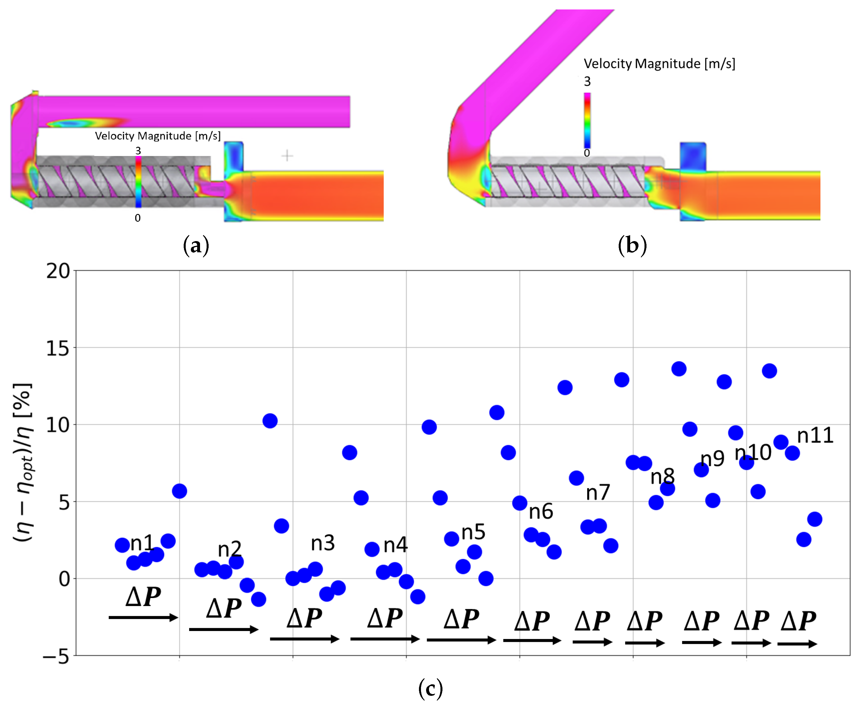
Furthermore, an advantageous aspect of transient CFD simulations is the capability to conduct an in-depth analysis of the machine, identifying turbulence or stall regions. In Figure 24a, the cross-sectional velocity magnitude is depicted at the high-speed high-pressure corner point, revealing noticeable recirculation areas leading to performance losses. The optimized geometry proposed in Figure 24b significantly mitigates this issue. For example, another insightful parameter to visualize for such a purpose could be turbulent kinetic energy (TKE). Figure 24c showcases the Experimental percentage efficiency improvement between the two proposed solutions across a wide range of pump speeds and discharge pressures. Clearly, a direct correlation is observed: the higher the speed, indicating increased recirculation, the greater the efficiency gain is. This serves as a compelling illustration of how such tools empower engineers to explore and implement effective solutions, strategically addressing specific challenges within the system.

Figure 24.
(a) Cross-section of velocity magnitude of the first design; (b) cross-section of velocity magnitude of optimized design; (c) Experimental percentual efficiency gain between the two designs.
4.5. Pressure Ripple
In this section, the outlet pressure ripple is compared against experiments and a numerical comparison for various circumferential gaps is presented. It is important to note that the volume of fluid (VOF) visualization presented in Figure 4a has been adapted in accordance with the methodology outlined in [48]. Specifically, a volume representing a constant diameter duct coupled with a calibrated orifice has been incorporated at the pump outlet to replicate a design that can be easily reproduced experimentally. It can be seen in Figure 25: in particular, Figure 25a shows the numerical VOF and exploits the positioning of the probing point, which replicates the position of the pressure sensor. Figure 25b shows the modified Experimental setup: it has to be noted that this design allows for the substitution of the manifold and the calibrated orifice representing the load according to any need.
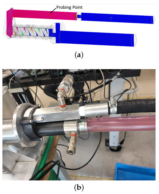
Figure 25.
(a) VOF of the updated model to investigate pressure ripple; (b) Experimental setup.
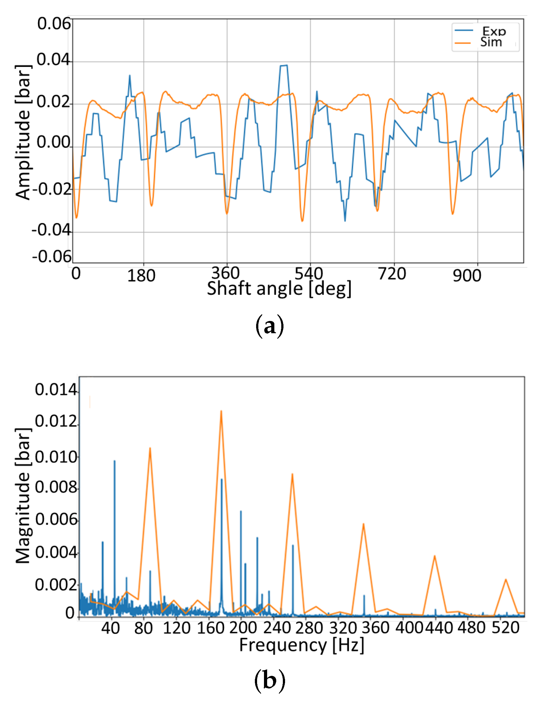
Figure 26 presents a comparison between numerical and Experimental pressure ripple in the time and frequency domain.

Figure 26.
Pressure ripple comparison: (a) time domain; (b) frequency domain.
Looking at the time domain signal, the numerical model predicts well the amplitude of the peak-to-peak signal. The shape is replicated quite well, although there are some differences. Since the driving spindle has two starts, their contribution during each pump’s revolution is visible. The fact that the Experimental ripple has a deeper dip suggests that the real engagement with the mating spindle is not as good. Also, some differences are due to geometrical errors that the real geometries carry. Looking at the frequency domain, despite some differences in magnitude, every component is predicted by the numerical models. In particular, it reveals the correlation of each frequency contribution to the geometrical parameters. Given the motor speed, the shaft frequency can be identified. It has to be noted that this frequency is only visible in the Experimental signal, also known as the whirl frequency, which is due to shaft misalignments and is not replicated by the numerical model.
Recalling that the driver spindle has 2 starts while the driven spindle has 3 starts, frequencies such as:
and their multiples such as:
can be clearly distinguished.
A numerical speculation concerning the pressure ripple for different circumferential gaps is presented in Figure 27. The amount of circumferential gap shown in Figure 26, denoted as Baseline, is increased by a factor of 2*Baseline and 4*Baseline. All simulations were conducted at a consistent speed of 2641 rev/min. Due to variations in the pump’s efficiency, the outlet average pressure marginally decreases from the Baseline model to the others with larger tolerances, indicating the presence of leakages.
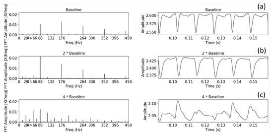
Figure 27.
Pressure ripple in time and frequency domains for: (a) Baseline; (b) 2*Baseline; (c) 4*Baseline.
The results encompass three pump revolutions, from the fifth to the eighth, to mitigate transient phenomena and attain quasi-static outcomes.
Notably, the 2f1 contribution predicted numerically is predominant in both the time and frequency domains, corresponding to the main spindle’s dual threads.
In terms of time domain results, the morphological similarity of the pressure ripples was evident when transitioning from the Baseline to the 2*Baseline configuration. Conversely, the 4*Baseline case exhibited distinct shapes, attributing to larger gaps and more-dominant leakages, making the kinematic machine ripple less pronounced. In this case, the contribution is spread across multiple frequencies, as observed in the frequency spectrum. To quantitatively assess the differences between models, it is common to refer to the NUG parameter as defined by [41] and reported in Table 4:
Table 4.
NUG parameter for the three presented models.
The reported NUG values highlight the noise emission potential of these machines, considering that the fluid-borne noise values arising from pressure ripples are limited.
5. Conclusions
In conclusion, this manuscript presents a thorough comparative analysis of simulation methodologies for spindle pumps. These machines have been chosen for their potential application in addressing the evolving needs of the automotive sector, particularly in the thermal management of Battery Electric Vehicles. The chosen reference machine, renowned for its high-efficiency characteristics and low noise emission capabilities, serves as a pertinent case study in this context.
5.1. Summary
The study involved the development of ad hoc simulation models using two primary modeling approaches—CFD and LP. Notably, an innovative approach for unsteady-CFD simulations was implemented using the commercial software Simerics MP+ (v6.0). Steady-CFD simulations, which allow for the prediction of leakage flow and pressure evolution, have been conducted using the commercial software Siemens Star-CCM+ (v.2206). Additionally, a novel LP simulation framework was formulated for screw pumps, featuring detailed Geometric, Force, and Fluid Dynamics Modules developed in Python and Simcenter Amesim (v.2021.2) environments, respectively. Importantly, for the first time, a Tool able to read the real geometry and extrapolate the needed for the Fluid Dynamics Module has been formulated for spindle pumps. The validation of the simulation models was rigorously conducted through an Experimental test campaign, involving the construction of several prototypes from scratch. The findings underscored the considerable potential held by LP models in analyzing such machines, outperforming both unsteady and steady CFD approaches in predicting steady characteristics. The appeal of LP models is further heightened by their limited computational time, aligning with the industry’s demand for fast and reliable tools in the early stages of machine design. Examining the steady-state results, it is noteworthy that the leakages exhibited non-speed dependence, and the pressure evolution over the spindles’ length followed a linear trend. The Torque analysis, encompassing a broad range of pump speeds and pressure drops, revealed a linear relationship with pressure, with speed-induced contributions more pronounced at extreme operational ranges. Specific considerations were identified for low- and high-speed operation, addressing potential issues related to increased friction. Spindle machines, known for their capability to handle fluids with larger air quantities, were assessed for aeration and cavitation phenomena. The study demonstrated how unsteady-CFD effectively handles such issues, pinpointing areas, such as interlope gaps and circumferential gaps, where aeration and cavitation are more likely to occur. A noteworthy contribution of this study is the numerical comparison of the pressure ripple for three different circumferential gaps in both the time and frequency domains. This analysis is crucial for the design of low-pressure pulsation pumps, aligning with the latest industry requirements. The study highlights the potential of spindle machines through the low values of the NUG parameter. In reflection, the authors affirm the high potential held by LP models, particularly for their modularity and efficiency in handling different aspects of spindle pump performance. Despite their advantages, it is acknowledged that the development effort required for such models can be substantial. Steady-CFD offers the advantage of predicting steady characteristics with limited effort, despite the high costs for the licenses. For a detailed analysis, unsteady-CFD emerged as the most-powerful Tool, providing users access to the highest level of detail, as discussed in the fluid dynamics optimization case.
5.2. Future Work
In future research endeavors, the focus could be directed toward refining and expanding LP models with submodels to address additional aspects, such as a dynamic Force Module that accounts for body motion, a transient Fluid Dynamics Module capable of predicting the pressure ripple, and a comprehensive Module able to analyze the way the fluid-borne noise interacts with the surface, aiming to ultimately predict and optimize the air-borne noise.
In essence, this study contributes valuable insights into the diverse simulation methodologies for spindle pumps, paving the way for advancements in the design and optimization of these machines, especially in the realm of automotive thermal management.
Author Contributions
Conceptualization, P.B. and E.F.; methodology, P.B. and E.F.; software, P.B. and E.F.; validation, P.B.; formal analysis, P.B. and E.F.; investigation, P.B.; resources, P.L., A.S. and E.F.; data curation, P.B.; writing—original draft preparation, P.B.; writing—review and editing, P.B. and E.F.; visualization, P.B.; supervision, P.L., A.S. and E.F.; project administration, P.L., A.S. and E.F.; funding acquisition, P.L., A.S. and E.F. All authors have read and agreed to the published version of the manuscript.
Funding
This research is part of a particular program, established by the Italian government, named PON Research & Innovation, where Italian Universities develop Ph.D. programs in collaboration with Italian firms and foreign universities. The parties involved in this program are the University of Naples Federico II, University of Sannio, Fluid-o-Tech, located in Corsico (MI), Italy, and the Maha Fluid Power Research Center, Purdue University (USA). Scolarship: DOT1318048–borsa n.1; CUP: E63D20002530006.
Data Availability Statement
All data generated for this manuscript are available in the text. Non-dimensional data have been chosen to respect confidentiality with the pump’s manufacturers.
Acknowledgments
First, the authors express gratitude to Federico Monterosso and Micaela Olivetti from Omiq Srl for their support in utilizing the software Simerics MP+. Special acknowledgment is extended to Fabrizio Tessicini from F-lab for his guidance and assistance with the commercial software Star-CCM+. The authors wish to acknowledge the noteworthy contribution of Mario Palomba, a former M.S. student of this research group, for his dedicated efforts in the development of the Fluid Dynamics Module within the Amesim environment. Sincere thanks are extended to Giuseppe Ricucci and Sabatino Iaumundo for their pivotal work in conducting the experiments and engaging in insightful discussions during the data analysis. Lastly, the authors express gratitude to Jacopo Varriale and Andrea Vecchio for their outstanding contributions to the design and manufacturing of the prototypes used in the Experimental test campaign. The authors also recognize the crucial contribution of Jacopo Varriale in the development and validation of the Force Module. The collective support, expertise, and dedication of these individuals and organizations have played a crucial role in shaping the outcomes of this research, and the authors are sincerely grateful for their contributions. The authors would like to express their gratitude for the valuable support provided by ChatGPT-3.5 in enhancing the written expression of this manuscript and proofreading the English.
Conflicts of Interest
Authors Pasquale Borriello and Pierpaolo Lucchesi were employed by the company Fluid-o-Tech s.r.l. The remaining authors declare that the research was conducted in the absence of any commercial or financial relationships that could be construed as a potential conflict of interest.
Abbreviations
| CFD | computational Fluid Dynamics |
| LP | lumped parameter |
| ICE | Internal Combustion Engine |
| BEP | Best Efficiency Point |
| PDM | positive displacement machine |
| PDEs | partial differential equations |
| FVM | finite-volume method |
| RANS | Reynolds-averaged Navier–Stokes |
| VOF | volume of fluid |
| CAD | Computer-Aided Design |
| TSV | Tooth Space Volume |
| EGM | External Gear Machine |
| DC | Displacement Chamber |
| NUG | Non-Uniformity Grade |
| BEV | Battery Electric Vehicle |
References
- Rodríguez, F. Fuel Consumption Simulation of HDVs in the EU: Comparisons and Limitations; ICCT: Washington, DC, USA, 2018. [Google Scholar]
- IEA. Global EV Outlook. 2021. Available online: https://www.iea.org/reports/global-ev-outlook-2021 (accessed on 16 December 2023).
- Mu, H.; Wang, Y.; Teng, H.; Jin, Y.; Zhao, X.; Zhang, X. Cooling system based on double-ball motor control valve. Adv. Mech. Eng. 2021, 13, 16878140211011280. [Google Scholar] [CrossRef]
- Mariani, L.; Di Bartolomeo, M.; Di Battista, D.; Cipollone, R.; Fremondi, F.; Roveglia, R. Experimental and numerical analyses to improve the design of engine coolant pumps. In Proceedings of the 75th National ATI Congress (ATI 2020), Rome, Italy, 15–16 September 2020; Volume 197, p. 06017. [Google Scholar]
- Li, W.; Lu, H.; Zhang, Y.; Zhu, C.; Lu, X.; Shuai, Z. Vibration analysis of three-screw pumps under pressure loads and rotor contact forces. J. Sound Vib. 2016, 360, 74–96. [Google Scholar] [CrossRef]
- Di Giovine, G.; Mariani, L.; Di Bartolomeo, M.; Di Battista, D.; Cipollone, R. Triple-screw pumps for ICE cooling systems in the transportation sector. In Proceedings of the National Congress of the ATI, Rome, Italy, 2–4 September 2021; Volume 312, p. 07024. [Google Scholar]
- Vetter, G.; Wincek, M. Performance prediction of twin screw pumps for two-phase gas/liquid flow. ASME. FED Am. Soc. Mech. Eng. Fluids Eng. Div. 1993, 154, 331–340. [Google Scholar]
- Vetter, G.; Wirth, W.; Korner, H.; Pregler, S. Multiphase pumping with twin-screw pumps-understand and model hydrodynamics and hydroabrasive wear. In Proceedings of the International Pump Users Symposium, Houston, TX, USA, 6–9 March 2000; pp. 153–170. [Google Scholar]
- Mewes, D.; Aleksieva, G.; Scharf, A.; Luke, A. Modelling twin-screw multiphase pumps—A realistic approach to determine the entire performance behaviour. In Proceedings of the 2nd International EMBT Conference, Hannover, Germany, 16–18 April 2008; pp. 104–116. [Google Scholar]
- Patil, A. Performance Evaluation and CFD Simulation of Multiphase Twin-Screw Pumps. Ph.D. Thesis, Texas A&M University, College Station, TX, USA, 2013. [Google Scholar]
- Chan, E. Wet-Gas Compression in Twin-Screw Multiphase Pumps. Ph.D. Thesis, Texas A&M University, College Station, TX, USA, 2010. [Google Scholar]
- Räbiger, K.E. Fluid Dynamic and Thermodynamic Behaviour of Multiphase Screw Pumps Handling Gas-Liquid Mixtures With Very High Gas Volume Fractions. Ph.D. Thesis, University of Glamorgan, Pontypridd, UK, 2009. [Google Scholar]
- Räbiger, K.; Maksoud, T.; Ward, J.; Hausmann, G. Theoretical and Experimental analysis of a multiphase screw pump, handling gas–liquid mixtures with very high gas volume fractions. Exp. Therm. Fluid Sci. 2008, 32, 1694–1701. [Google Scholar] [CrossRef]
- Feng, C.; Yueyuan, P.; Ziwen, X.; Pengcheng, S. Thermodynamic performance simulation of a twin-screw multiphase pump. Proc. Inst. Mech. Eng. Part E J. Process. Mech. Eng. 2001, 215, 157–163. [Google Scholar] [CrossRef]
- Hu, B.; Cao, F.; Yang, X.; Wang, X.; Xing, Z. Theoretical and Experimental study on conveying behavior of a twin-screw multiphase pump. Proc. Inst. Mech. Eng. Part E J. Process. Mech. Eng. 2016, 230, 304–315. [Google Scholar] [CrossRef]
- Liu, P.; Patil, A.; Morrison, G. Multiphase flow performance prediction model for twin-screw pump. J. Fluids Eng. 2018, 140, 031103. [Google Scholar] [CrossRef]
- Ransegnola, T.; Zappaterra, F.; Vacca, A. A strongly coupled simulation model for external gear machines considering fluid-structure induced cavitation and mixed lubrication. Appl. Math. Model. 2022, 104, 721–749. [Google Scholar] [CrossRef]
- Ma, R.; Wang, K. CFD numerical simulation and Experimental study of effects of screw-sleeve fitting clearance upon triangular thread labyrinth screw pump (LSP) performance. J. Appl. Fluid Mech. 2010, 3, 77–81. [Google Scholar]
- Tang, Q.; Zhang, Y.; Pei, L.; Tang, J. Optimal design of screw and flow field analysis for twin-screw pump. In Proceedings of the ASME 2011 International Design Engineering Technical Conferences and Computers and Information in Engineering Conference, Washington, DC, USA, 29–31 August 2011; Volume 54853, pp. 593–600. [Google Scholar]
- Tang, Q.; Zhang, Y. Screw optimization for performance enhancement of a twin-screw pump. Proc. Inst. Mech. Eng. Part E J. Process. Mech. Eng. 2014, 228, 73–84. [Google Scholar] [CrossRef]
- Kovacevic, A.; Stosic, N.; Smith, I. Screw Compressors: Three Dimensional Computational Fluid Dynamics and Solid Fluid Interaction; Springer Science & Business Media: Berlin/Heidelberg, Germany, 2007; Volume 46. [Google Scholar]
- Stosic, N.; Smith, I.; Kovacevic, A. Screw Compressors: Mathematical Modelling and Performance Calculation; Springer Science & Business Media: Berlin/Heidelberg, Germany, 2005. [Google Scholar]
- Mujic, E.; Kovacevic, A.; Stosic, N.; Smith, I. Advanced design environment for screw machines. In Proceedings of the 20th International Compressor Engineering Conference, West Lafayette, IN, USA, 12–15 July 2010. [Google Scholar]
- Lu, Y.; Kovacevic, A.; Read, M.; Basha, N. Numerical study of customised mesh for twin screw vacuum pumps. Designs 2019, 3, 52. [Google Scholar] [CrossRef]
- Yan, D.; Kovacevic, A.; Tang, Q.; Rane, S. Numerical investigation of cavitation in twin-screw pumps. Proc. Inst. Mech. Eng. Part C J. Mech. Eng. Sci. 2018, 232, 3733–3750. [Google Scholar] [CrossRef]
- Borriello, P.; Frosina, E.; Senatore, A.; Monterosso, F. Numerical Modelling and Experimental Validation of Twin-Screw Pumps Based on Computational Fluid Dynamics using SCORG® and SIMERICS MP+®. In Proceedings of the 76th Italian National Congress ATI (ATI 2021), Rome, Italy, 2–4 September 2020; Volume 312, p. 05007. [Google Scholar]
- Moghaddam, A.H.; Kutschelis, B.; Holz, F.; Börjesson, T.; Skoda, R. Three-Dimensional Flow Simulation of a Twin-Screw Pump for the Analysis of Gap Flow Characteristics. J. Fluids Eng. 2022, 144, 031202. [Google Scholar] [CrossRef]
- Simerics MP+ Version 6.0.4. Available online: https://www.simerics.com/libraries (accessed on 18 December 2023).
- Singhal, A.K.; Athavale, M.M.; Li, H.; Jiang, Y. Mathematical basis and validation of the full cavitation model. J. Fluids Eng. 2002, 124, 617–624. [Google Scholar] [CrossRef]
- Vacca, A.; Guidetti, M. Modelling and Experimental validation of external spur gear machines for fluid power applications. Simul. Model. Pract. Theory 2011, 19, 2007–2031. [Google Scholar] [CrossRef]
- Yan, D.; Tang, Q.; Kovacevic, A.; Rane, S.; Pei, L. Rotor profile design and numerical analysis of 2–3 type multiphase twin-screw pumps. Proc. Inst. Mech. Eng. Part E J. Process. Mech. Eng. 2018, 232, 186–202. [Google Scholar] [CrossRef]
- Simcenter Amesim, Hydraulic Library User’s Guide, Version 2022.1. 2022. Available online: https://plm.sw.siemens.com/en-US/simcenter/systems-simulation/amesim/ (accessed on 19 December 2023).
- Vacca, A.; Franzoni, G. Hydraulic Fluid Power: Fundamentals, Applications, and Circuit Design; John Wiley & Sons: Hoboken, NJ, USA, 2021. [Google Scholar]
- Mistry, Z.; Vacca, A. Cavitation Modeling Using Lumped Parameter Approach Accounting for Bubble Dynamics and Mass Transport Through the Bubble Interface. J. Fluids Eng. 2023, 145, 081401. [Google Scholar] [CrossRef]
- Pellegri, M.; Manne, V.H.B.; Vacca, A. A simulation model of Gerotor pumps considering fluid–structure interaction effects: Formulation and validation. Mech. Syst. Signal Process. 2020, 140, 106720. [Google Scholar] [CrossRef]
- Mistry, A.Z.; Vacca, K.U. Modeling and Experimental Validation of Twin Lip Balanced Vane Pump Considering Micromotions, Contact Mechanics, and Lubricating Interfaces. Simul. Model. Pract. Theory 2023. accepted. [Google Scholar]
- Marinaro, G.; Frosina, E.; Senatore, A. A numerical analysis of an innovative flow ripple reduction method for external gear pumps. Energies 2021, 14, 471. [Google Scholar] [CrossRef]
- Mazzei, P.; Frosina, E.; Senatore, A. Helical Gear Pump: A comparison between a lumped parameter and a computational Fluid Dynamics-based approaches. Fluids 2023, 8, 193. [Google Scholar] [CrossRef]
- Rituraj, R.; Vacca, A. Investigation of flow through curved constrictions for leakage flow modelling in hydraulic gear pumps. Mech. Syst. Signal Process. 2021, 153, 107503. [Google Scholar] [CrossRef]
- Merritt, H.E. Hydraulic Control Systems; Wiley: Hoboken, NJ, USA, 1967. [Google Scholar]
- Ivantysyn, J.; Ivantysynova, M. Hydrostatic Pumps and Motors: Principles, Design, Performance, Modelling, Analysis, Control and Testing; Tech Books International: New Delhi, India, 2003. [Google Scholar]
- Koplin, C.; Abdel-Wahed, S.A.; Jaeger, R.; Scherge, M. The transition from static to dynamic boundary friction of a lubricated spreading and a non-spreading adhesive contact by macroscopic oscillatory tribometry. Lubricants 2019, 7, 6. [Google Scholar] [CrossRef]
- Di Giovine, G.; Mariani, L.; Di Battista, D.; Cipollone, R.; Fremondi, F. Modeling and Experimental validation of a triple-screw pump for internal combustion engine cooling. Appl. Therm. Eng. 2021, 199, 117550. [Google Scholar] [CrossRef]
- Reitschuster, S.; Maier, E.; Lohner, T.; Stahl, K. Friction and temperature behavior of lubricated thermoplastic polymer contacts. Lubricants 2020, 8, 67. [Google Scholar] [CrossRef]
- Maitra, G.M. Handbook of Gear Design; CRC Press: Boca Raton, FL, USA, 1994. [Google Scholar]
- Houpert, L. An engineering approach to Hertzian contact elasticity—Part I. J. Trib. 2001, 123, 582–588. [Google Scholar] [CrossRef]
- Borriello, P.; Frosina, P.E.; Lucchesi, A.S. A Study on a Twin-Screw Pump for Thermal Management Systems by means of CFD using SimericsMP+®: Experimental validation and focus on Pressure Pulsation. IEEE 2022. accepted. [Google Scholar]
- Frosina, E.; Marinaro, G.; Senatore, A. Experimental and numerical analysis of an axial piston pump: A comparison between lumped parameter and 3D CFD approaches. In Proceedings of the Fluids Engineering Division Summer Meeting. American Society of Mechanical Engineers, San Francisco, CA, USA, 28 July–1 August 2019; Volume 59025, p. V001T01A042. [Google Scholar]


Disclaimer/Publisher’s Note: The statements, opinions and data contained in all publications are solely those of the individual author(s) and contributor(s) and not of MDPI and/or the editor(s). MDPI and/or the editor(s) disclaim responsibility for any injury to people or property resulting from any ideas, methods, instructions or products referred to in the content. |
© 2024 by the authors. Licensee MDPI, Basel, Switzerland. This article is an open access article distributed under the terms and conditions of the Creative Commons Attribution (CC BY) license (https://creativecommons.org/licenses/by/4.0/).