Abstract
We present an analysis of the effect of particle inertia and thermal inertia on the heat transfer in a turbulent shearless flow, where an inhomogeneous passive temperature field is advected along with inertial point particles by a homogeneous isotropic velocity field. Eulerian–Lagrangian direct numerical simulations are carried out in both one- and two-way coupling regimes and analyzed through single-point statistics. The role of particle inertia and thermal inertia is discussed by introducing a new decomposition of particle second-order moments in terms of correlations involving Lagrangian acceleration and time derivative of particles. We present how particle relaxation times mediate the level of particle velocity–temperature correlation, which gives particle contribution to the overall heat transfer. For each thermal Stokes number, a critical Stokes number is individuated. The effect of particle feedback on the attenuation or enhancement of fluid temperature variance is presented. We show that particle feedback enhances fluid temperature variance for Stokes numbers less than one and damps is for larger than one Stokes number, regardless of the thermal Stokes number, even if this effect is amplified by an increasing thermal inertia.
1. Introduction
The interaction between inertial heavy particles and the dynamic and thermal fields of turbulent fluid spans multiple scales and influences many natural and industrial phenomena. This interplay significantly shapes the evolution of dynamic systems in both natural and industrial settings. Understanding this complex flow regime is pivotal for designing more efficient energy conversion systems, refining weather prediction tools, addressing plastic particle pollution in oceans, enhancing air quality, and advancing our understanding of cloud physics. The dynamics of single-phase turbulent flows with temperature transport is, per se, a complex problem which has been under investigation for decades. The presence of inertial particles adds further complexity, especially in regimes where fluid–particle thermal interaction occurs. Although passive scalar and particle transport in turbulent flows has been studied since the pioneering work of Taylor [1] and Kraichnan [2], the problem which involves the coupled dynamical and thermal interaction of an inertial particle with turbulent fields is relatively new and has garnered limited attention in past research.
Direct experimental measurements in particle-laden flows, especially considering thermal interactions between fluid and particles, pose significant challenges. Therefore, the few experimental studies have relied on techniques like PIV (particle image velocimetry) and PTV (particle tracking velocimetry) to gather bulk statistics of fluid and suspended particles. For instance, recent research has explored near-wall particle interaction in wall-bounded flows [3,4], investigated gas–particle turbulent flow using two-colour laser-induced fluorescence (LIF) to gauge fluid temperature statistics under high radiative flux [5] and studied the effect of particle preferential concentration on fluid temperature statistics in turbulent square duct flow by altering radiative heat flux absorption [6]. A priori statistical approaches to these flows, mostly base on the stochastic theory, offer valuable insight under specific ad hoc assumptions. For instance, kinetic theory is used to derive the single-particle or fluid–particle pdf transport equation, along with proposing two-phase Eulerian–Eulerian macroscopic field equations and some closure models [7,8,9].
Therefore, performing high fidelity numerical simulation can fill the gap, offering detailed temperature statistics for both phases and enabling a deeper understanding of thermal transport in a turbulent flow seeded with particles. Advancements in high-performance computing have provided researchers with powerful computing capabilities for simulation-assisted analysis of turbulence, allowing direct numerical simulations (DNSs). Many studies on particle-laden flows in non-homothermal systems have focused on channel flow, due to the importance of wall-bounded flows. Zonta et al. [10] observed enhanced heat transfer for small particles and reduced transfer for very large ones at a fixed Prandtl number and volume fraction. Kuerten et al. [11] found that inertial particles with a high specific heat capacity augment heat transfer due to the preferential concentration in near-wall regions, a phenomenon known as turbophoresis. Nakhaei et al., 2017 [12] explored the impact of very large inertial particles and high volume fractions at a fixed volume fraction and particle-to-fluid specific heat, revealing a reduction in convective turbulent heat flux compared to unseeded flow, attributed to increased heat exchange between the carrier flow and the suspended particles, and less-efficient fluid–particle heat transfer in the near-wall region, reducing turbopheresis. Lessani et al. [13] found that heat transfer from the solid wall increases proportionally with the thermal Stokes number when the mass loading and particle Stokes number are fixed, but there is also a reduction in convective turbulent Nusselt number with an increase in particle thermal Stokes number, holding volume fraction and particle Stokes number constant.
Other works have numerically studied the modulation of heat transfer by the presence of inertial particles in homogeneous isotropic turbulent flows, the fundamental archetype of most theoretical studies on turbulence. Pouransari et al. [14,15] investigated particle-to-fluid heat transfer in a compressible flow at low Mach numbers. They found a strong dependence of particle-to-fluid heat transfer on Stokes number and particle spatial distribution, with a weak dependence on flow Reynolds number and particle-to-fluid heat capacity ratio. From DNS data they developed a small-scale phenomenological model able to capture clustering effects on heat transfer, introducing a timescale for particle modulation of fluid temperature in the two-way coupling regime. More recently, Carbone et al. [16] carried out a comprehensive study on multiscale fluid–particle thermal interaction. They demonstrated a monotonic decrease in fluid temperature variance with particle thermal relaxation time. Additionally, their results showcased that, while the probability density function (PDF) of the fluid temperature gradient scales with its variance, the PDF of particle thermal acceleration does not scale self-similarly but shows multi-fractality at small-scales. The study highlighted the significant role of particle velocity alignment with local fluid temperature gradient in fluid temperature front clustering. Moreover, they elucidated the suppression of fluid temperature increments by particle thermal feedback with increasing particle inertia and offered statistical analyses characterizing particle thermal caustics and non-local thermal behavior. Saito et al. [17] extended this analysis, utilizing a Langevin equation to model fluid temperature fluctuations seen by particles. These results align with Béc et al.’s analysis [18], showcasing strong fluid–particle coupling at small scales, where particles tend to concentrate in high scalar gradient regions, experiencing strong temperature fluctuations along their Lagrangian trajectory due to intermittency. Moreover, ref. [18] used particle thermal acceleration variance as a measure for particle heat flux, providing its scaling laws in terms of thermal Stokes number for low and high particle thermal inertia.
Although these works have analyzed in detail the multiscale fluid–particle thermal interactions, they have only considered a situation of isotropic and statistically steady flow. In our recent studies [19,20], we quantified the particle contribution to heat transfer in the simplest thermally inhomogeneous flow generated by a temperature step between two homothermal regions advected by a homogeneous and isotropic velocity field. We analyzed the role of particles across a wide range of Stokes numbers in one- and two-way coupling regimes. During an almost self-similar stage of evolution of the thermal interaction region, we observed the maximum particle contribution to heat flux at a Stokes number around one, corresponding to particle maximum clustering regardless of particle thermal capacity, although the latter determined the maximum. However, particle feedback tended to damp temperature fluctuations, reducing the transport by turbulent fluid flows fluctuations. Furthermore, in subsequent works [21,22] we explored the effect of inter-particle collisions. Collisions primarily influence the flow through particle back-reaction on fluid temperature fields, as the particle scattering induced by a collision increases the fluid–particle temperature difference and reduces the particle temperature–velocity correlation. Nevertheless, the overall impact on all statistics is very mild at the volume fraction where the point-particle model in the one- and two-way coupling regimes is valid.
In the present study, we extend our previous works [20,21] with the aim to analyze the effect of particle thermal inertia independently from particle inertia, that is, we treat the momentum and thermal relaxation times as independent parameters. This is unlike previous studies in which they are always proportional to each other, so that both effects can be individually accounted for. For simplicity and to concentrate on particle inertia, we consider a single Reynolds number, reducing the number of parameters. Our primary objective in this work is to elucidate and characterize the influence of particle inertia and thermal inertia on the turbulent heat flux, identifying also the behaviour of the particles in the different limiting conditions. To this purpose, our analysis primarily focuses on examining the temperature variance and the velocity–temperature correlation, which provides the convective heat flow, in the mixing layer. We introduce a novel decomposition of these moments, using correlations involving particle acceleration and the derivative of their temperature. This reveals how particle acceleration, mediated by the relaxation times, influences the heat flux. Acceleration statistics have been shown to be a powerful tool to unravel non-trivial aspects of both fluid and particle dynamics, highlighting the limits of existing models [23,24]. The physical model of the problem we tackle is described in Section 2, together with the flow configurations and the numerical method used in the simulations. In Section 3, the results of the simulations are presented and discussed and fluid and particle statistics are reported in terms of a various range of simulated Stokes number and thermal Stokes. The flow configuration presented in this work is the only thermally inhomogeneous particle-laden flow, apart from channel flow, which has been investigated by means of direct numerical simulations. Notwithstanding its apparent simplicity, it presents a number of non-trivial results that can be useful to interpret more complex flows. For example, the heat transfer and mixing properties observed in this type of inhomogeneous flow also play a significant role in cloud edge dynamics, where a humidity gradient is associated with a temperature gradient (e.g., [25,26]).
2. Physical Model
We consider a fluid seeded by a large number of identical small particles. When particle size is much smaller than any relevant flow scale and their volume fraction is very small, the Eulerian–Lagrangian point-particle model is an appropriate tool to describe their dynamics. In this approach, the carrier flow is described by the Navier–Stokes equations in spatial Eulerian coordinates, while particles are singularly tracked. That is, the dynamics of the incompressible carrier flow is described by
where , and are the velocity, pressure and temperature fields; is the fluid density and and are the isobaric specific heat capacity and fluid kinematic viscosity, respectively. Field is an external body force introduced to maintain turbulent fluctuations in a statistically steady state and is the heat exchanged per unit time and unit mass with particles, i.e., particle thermal feedback on the carrier flow. Similar to previous works (e.g., [20,21,22]), we do not consider the force exerted by particles on the fluid: only the fluid temperature field is two-way coupled with particles, and momentum exchange occurs only under one-way coupling regime. This assumption yields a dilute regime in our problem because it has been found that momentum feedback has a minor thermal effect on fluid temperature statistics [16].
We assume that the flow is seeded by a monodisperse suspension of identical spherical particles of radius R, density and isobaric specific heat capacity . Particles are regarded as material points, with a radius much smaller than carrier flow Kolmogorov lenghtscale and a density much higher than the fluid density, thus obeying the simple equation of motion proposed by Gatignol [27] and Maxey and Riley [28]. Under these conditions, the Stokes drag force is the dominant term in the Maxey–Riley equation, and all other force terms, as well as terms linked to the flow inhomogeneity in the neighborhood of each particle, are neglected. An analogous equation for the particle temperature is derived under the same hypothesis, so that the dynamics of each individual particle is governed by the following equations in the Lagrangian reference frame
where , and are position, velocity and temperature of the p-th particle, respectively, and define the state of the particle. Here, and are the momentum and thermal relaxation times, given by
where the velocity and temperature of the carrier flow, and , are evaluated in correspondence of the position of the particle. Any direct particle–particle interaction is excluded, so that particles can interact only indirectly by altering the carrier flow dynamics through the thermal feedback in Equation (3), which is thus given by the heat transferred by particles to the fluid per unit volume and unit time, i.e.,
where is the total number of spherical inertial particles seeding the carrier fluid and is the Dirac delta function. In the one-way coupling regime, this thermal feedback is not considered, and is set equal to zero.
In this study we use this physical model to investigate the heat transfer between two regions with different uniform temperatures, and , within a homogeneous and isotropic velocity field, as in [20,22]. Therefore, the governing equations are numerically solved in a parallelepiped computational domain, with Cartesian coordinates , defined by , and , where is the domain length in directions and and is the length in direction . In the following, as in [20], we chose to set in order to avoid constraining the process, which ideally occurs in an infinite domain, through the computational domain size.
The temperature distribution is initialized by setting the temperature equal to in the half-domain where and to in the half-domain where . To avoid numerical issues, the discontinuity at is smoothed with a hyperbolic tangent [20]. The initial fluid velocity field is obtained from a dedicated simulation of homogeneous and isotropic turbulence, carried out until a statistically steady state is reached. A large-scale low wavenumber forcing, linear function of the current velocity, is applied as in [16,20].
The carrier flow Equations (1)–(3) are solved with a Fourier–Galerkin method, so that periodic boundary conditions are imposed on all faces of the computational domain, as customary in the directions where a turbulent flow is statistically homogeneous. However, temperature is intrinsically not periodic in this flow, so that it is decomposed into a steady mean linear field and a residual part,
where the origin is taken in the centre of the domain, so that periodic boundary conditions can be applied to the residual part , as described in detailed in [20]. The same decomposition is applied to the particle temperature, i.e.,
For the sake of consistency with the physics of the two-phase flow and with the boundary conditions of the fluid phase, any particle that may exit the computational domain is reintroduced on the opposite side with the same velocity and residual temperature .
A fully dealiased pseudospectral method, using the 3/2-rule, is employed to discretize the spatial domain of the fluid phase equations [29], while the interpolation of fluid velocity and temperature at particle positions, and computation of the particle thermal feedback (6), is carried out using a recent numerical method [30,31] based on inverse and forward non-uniform fast Fourier transforms with a fourth-order B-spline basis. Since the forcing determines the mean dissipation rate in statistically steady conditions, the Kolmogorov microscale is known in advance, while the integral scale is determined by the forced wavenumber (see Appendix A and [16] for further details on the forcing). All simulations have been carried out on a grid in the Fourier space, which becomes in the physical space to compute the nonlinear terms and particles interpolations and feedback according to the 3/2-rule. Having set the resolution such that , where is the mesh spacing in physical space ( if the 3/2-rule finer grid is considered), the method allows accurate interpolation in the physical space and an accurate spectral representation of the thermal feedback (see [30] for the evaluation of the errors). Integration in time was performed for both the carrier flow Equations (1)–(3) and the particle Equation (4) using a second-order exponential integrator.
The governing Equations (1)–(6) are solved in dimensionless form, normalizing them by using the size of the domain in the homogeneous direction, , as reference length, a reference velocity deduced from the imposed mean kinetic energy dissipation rate through the body force (see [16]) and the temperature difference as reference temperature [20]. That is, we define
The dimensionless form of the governing Equations (1)–(4) is in Appendix A. In the dimensionless form, the flow is governed by the Reynolds number , the Prandtl number and the particle-to-fluid heat capacity ratio , where is the particle volume fraction, while particle dynamics are described by the Stokes numbers, which represent the ratio between their relaxation times and the flow timescales (see Appendix A). Given the arbitrariness of the length scale , the flow is more conveniently and usually described by the Taylor microscale Reynolds number , where is the Taylor microscale, while the Kolmogorov timescale , which is the smallest timescale of the flow and characterizes the small-scale velocity fluctuations of the fluid phase, will be used as a reference timescale to normalize instead of the large-scale time of the adimensionalization. Thus, the Stokes number and the thermal Stokes number are used to describe the particle’s dynamic and thermal behaviour.
3. Results and Discussion
In this section a few aspects of the role of particles in the thermal interaction between two homothermal regions, advected by a statistically steady homogeneous and isotropic velocity field, will be discussed from the data obtained from a set of direct numerical simulations. Given the large set of parameters, the discussion will focus on the role of particle inertia, and not on the Reynolds and Prandtl numbers or on the volume fraction. Therefore, all simulations have been carried out at the same Taylor microscale Reynolds number , at a fixed Prandtl number . Particle volume fraction has been set equal to in all the simulations. The density ratio is set as , corresponding to the one of water particles in air, so that particle relaxation times are varied by changing the particle size and the specific heat ratio between the particles and fluid. Anyway, only the relaxation times of particles matter, and the values of a particle’s parameters have been chosen such that we could explore the behaviour of the system for Stokes numbers up to 6 and thermal Stokes numbers up to 10 in both the one- and two-way coupling regimes. However, differently from previous studies on this problem [19,20,22] which kept the ratio constant, we consider inertia and thermal inertia as independent parameters, thus St and are varied independently.
The interface which initially separates the two homothermal regions is spread by the turbulent velocity field and evolves into a thermal mixing layer characterized by a high temperature variance and a strong intermittency at its borders [32]. As we have shown in [20], the region where the temperature is not uniform and the two zones interact has a thickness which grows in time and, after a few eddy turnover times , where ℓ is the integral scale of the flow and the root mean square of velocity fluctuations, the mean temperature of the fluid shows, up to the numerical uncertainty, a self-similar profile. This allows us to define a measure of the thickness of the interaction layer from the mean temperature of the carrier fluid as
to be used as the length scale of the layer [20]. When the fluid and particle second-order moments are rescaled using the temperature difference and the thickness as scales, all profiles tend to collapse into a single curve, i.e., this interaction zone develops in a self-similar way, up to the numerical uncertainty. This lengthscale shows a diffusive growth. Particles which move across this non-homothermal layer experience a strong mean temperature gradient, leading to high temperature derivatives, whose distribution is strongly intermittent with large non-Gaussian tails.
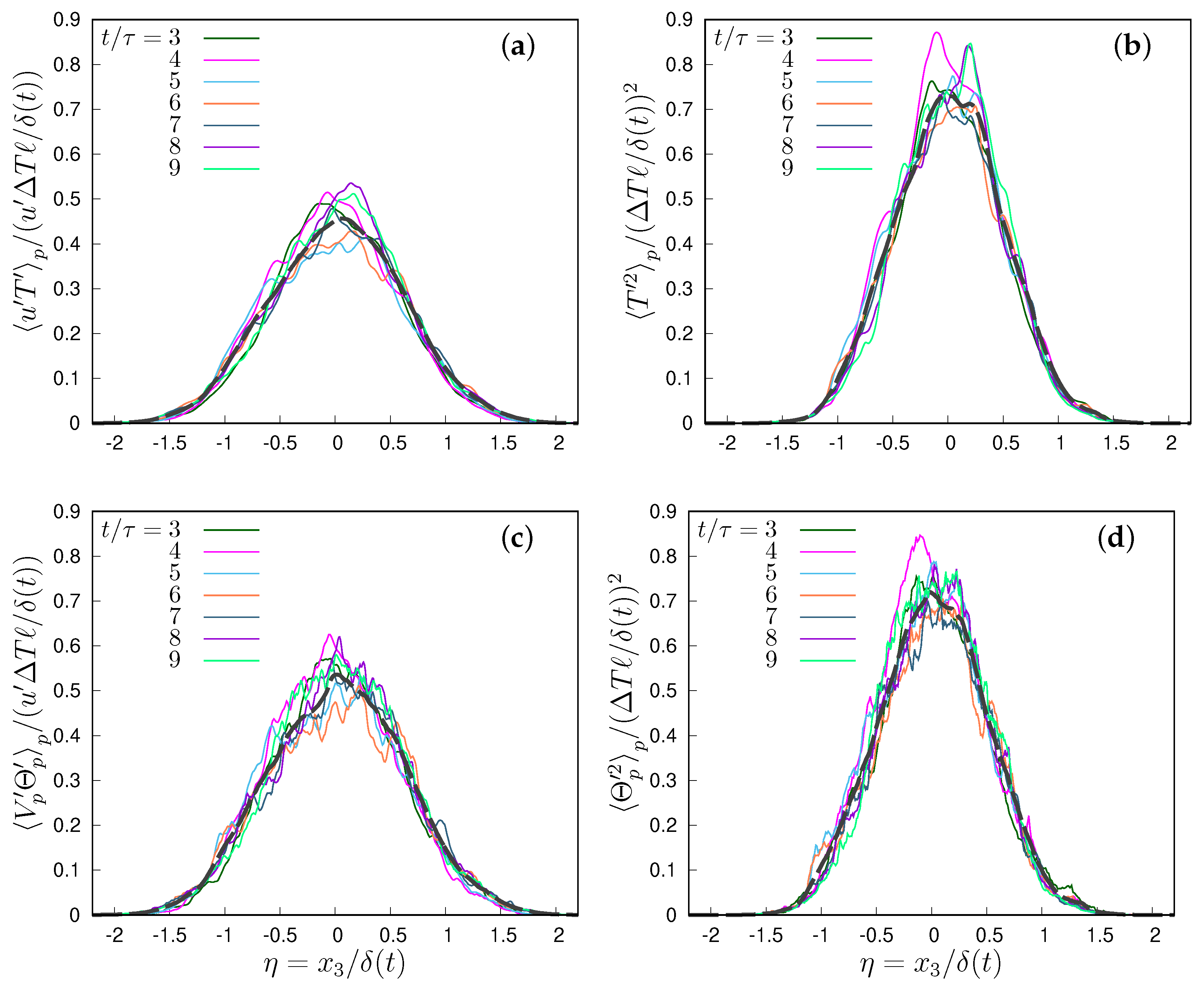
Figure 1 shows an example of spatial distribution of the convective heat flux and the particle temperature variance, normalized with the mixing layer thickness , when . Both the variance and the temperature–velocity correlation have a maximum for , where the mean temperature gradient is largest. The temperature gradient across the mixing layer is of order , so that the large scales of the flow, of the order of the integral scale ℓ, perceive a temperature difference of order , which is the expected scale of temperature fluctuations inside the mixing layer. Therefore, if is the root mean square of the fluid velocity fluctuations, the correlation can dimensionally scale only as , while the temperature variance should scale as . All the curves of both moments are very close for , almost collapsing within the limits of the noise associated with their computation. This also implies a self-similar or almost self-similar behaviour of particle second-order moments, a feature already observed in [20]. Therefore, it is possible to average in time all the rescaled moments. In the following, we will discuss the properties of the mixing layer by considering all moments in the centre of the mixing layer. Given the almost self-similar behaviour, this is representative of the entire layer.
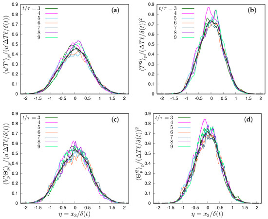
Figure 1.
(a,c) Rescaled convective fluid and particle heat flux (temperature–velocity correlation) and (b,d) re-scaled fluid and particle temperature variance. Both the Stokes number and the thermal Stokes number are equal to 1 in this example. In all panels, and the dashed lines indicate the time average of the re-scaled variables for .
This interaction or, broadly speaking, thermal mixing layer (in the sense of [20,32,33]) is characterized also by the onset of a significant velocity–temperature correlation, which is responsible for most of the transfer of enthalpy across the layer, since, by averaging Equation (3), the mean heat flux in the inhomogeneous direction is given by
or, in dimensionless form (see Appendix A for the dimensionless form of the equations according to the adimensionalization (7)),
where the first term is the mean temperature diffusion, the second the convective heat flux and the third the particle contribution to the mean heat transfer. Since is the only length-scale of the problem, is the scale of the heat flux in static conditions. A Nusselt number can be defined as the ratio between this flux, computed in the mixing centre, and . By using the definition of , Equation (8), this is equal to the diffusive term in (9) when the flux is computed in the mixing centre, so that the Nusselt number is
Therefore, the re-scaled fluid and particle temperature–velocity correlation, see, e.g., Figure 1a, give just the fluid and particle contribution to the Nusselt number of this flow configuration.
Particles have a dual role in the interaction between the two regions, which globally manifests itself with a transfer of heat from one to the other: a direct role, as their motion counteracts the enthalpy transfer, and an indirect role, due to the modulation of temperature and velocity fluctuations of the carrier fluid. Therefore, both one- and two-way thermally coupled regimes are considered, because their differences allow to evidence the role of particle feedback in the flow, i.e., the indirect role of particles. Since the coupling between the convective heat transfer and particles creates a very complex scenario, as stated in Section 2, we do not consider the particle momentum feedback, which has a minor role [15,16,17] in homogeneous flows, and neither do we consider collisions between particles, whose effect have been documented in [21,22].
3.1. Temperature and Velocity Moments in Terms of Particle Time Derivatives
Given the flow inhomogeneity and unsteadiness, in the following we consider conditional averages at a given time and position along the inhomogeneous direction, i.e., we define, for any function f of the state of the particle,
where is the statistical average and we define the fluctuation of f as . We will now express the average temperature fluctuations and the heat flux in terms of the time derivatives of particle velocity (i.e., the acceleration) and temperature. By subtracting from (4) its conditional average, the particle temperature and velocity fluctuations can be expressed in terms of the fluctuations of the time derivatives, i.e.,
where fluid velocity and temperature are to be computed at particle position. In the following, we will skip the apex from all moments that are second order or higher to keep notations simple. By multiplying the particle temperature fluctuation (12) equation by and and conditionally averaging, we have
Therefore, the ratio of particle temperature variance to fluid temperature variance at particle position is
while, by multiplying (12) by the temperature derivative and conditionally averaging, we have instead a relation for the variance of the temperature derivative,
Equations (15) and (16) are general and can help to analyze the role of particle thermal inertia in the fluid and particle temperature statistics. Given the self-similarity of the flow [20], this ratio is independent from the position and time t. In the following, we will use it to discuss the behaviour of the flow in the central region of the mixing layer, in a thin region, of a thickness much less than , where variance and heat flux have their maximum [20]. All data presented in the figures refer to this zone, because the relative homogeneity of the flow in this zone [32] allows for the reduction in noise in the processing of numerical data.
A few pieces of information can be directly inferred from these equations, in particular as regards the limiting cases. In the zero-thermal inertia limit, , particle temperature variance and fluid temperature variance become the same, independently from the momentum relaxation time. On the other hand, in the opposite limit , the ratio is equal to . This shows the importance of particle temperature derivatives in the determination of particle temperature fluctuations. As discussed by Carbone et al. [16] and Béc et al. [18], particle thermal acceleration is responsible for particle–fluid small-scale thermal coupling even in the one-way coupling regime.
Indeed, they discussed the small-scale fluid–particle interaction on the basis of the statistics of the particle thermal acceleration in one- and two-way coupling, leading to the conclusion that particle inertia generates a multifractal behaviour, as indicated by Lagrangian temperature structure functions. Such a lack of smoothness, defined by [16] as thermal caustics, dominates at small scales, where particle temperature differences at small separation rapidly increase as the Stokes number and the thermal Stokes number are increased. Béc et al. [18] related the onset of the fluid temperature fronts along a particle’s Lagrangian path to the dynamics of particle temperature acceleration, whose non-Gaussian statistics leads to multifractal behaviour. Note that at a fixed Stokes number we can use (14) to understand the effect of particle thermal inertia at a very high thermal Stokes number. Even if particle inertia does not appear explicitly in Equations (13)–(15), inertia influences particle trajectories and therefore the fluid temperature at a particle’s position.
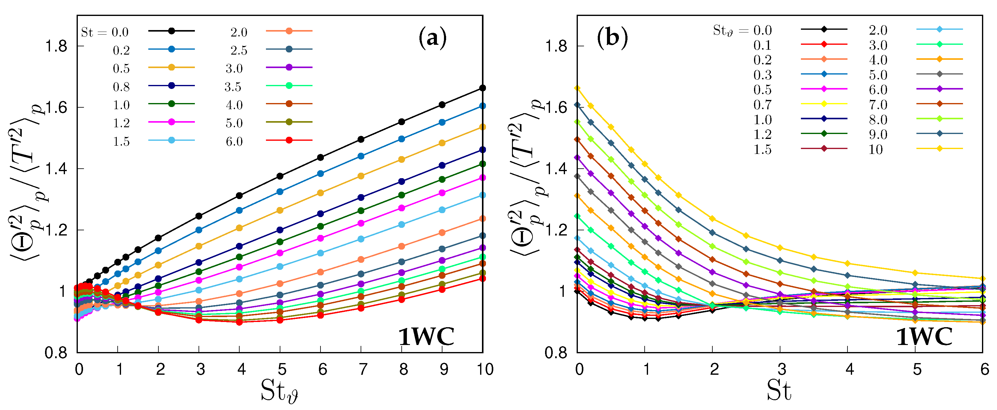
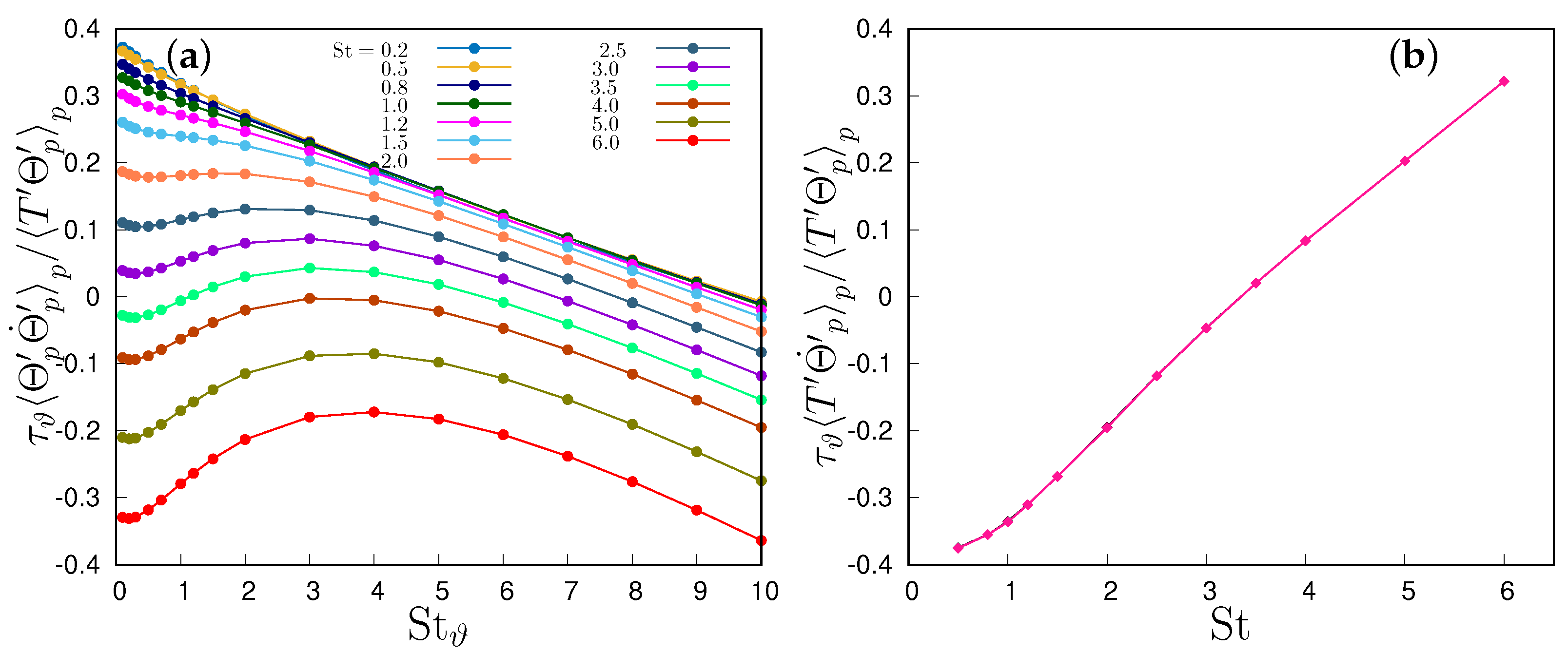
Figure 2a shows that the ratio of variances increases with for any Stokes number at large , i.e., at least when , but the slope reduces at higher inertia, so that at fixed , Figure 2b, it always reduces if . On the contrary, at low thermal inertia, , particle temperature variance always remains lower than fluid temperature variance and approaches it in the limit. In the one-way coupling regime, the denominator of (15) is a function of St only, and increases with St (Figure 3b) so that the thermal inertia acts only on in the numerator (Figure 3a).
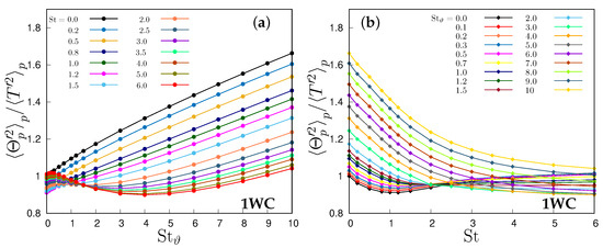
Figure 2.
Ratio between particle temperature variance to fluid temperature variance in one-way coupling simulations, (a) as a function of the thermal Stokes number and (b) as function of the Stokes number.
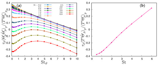
Figure 3.
Normalized particle temperature derivative correlation with (a) particle temperature and (b) fluid temperature. One-way coupling regime.
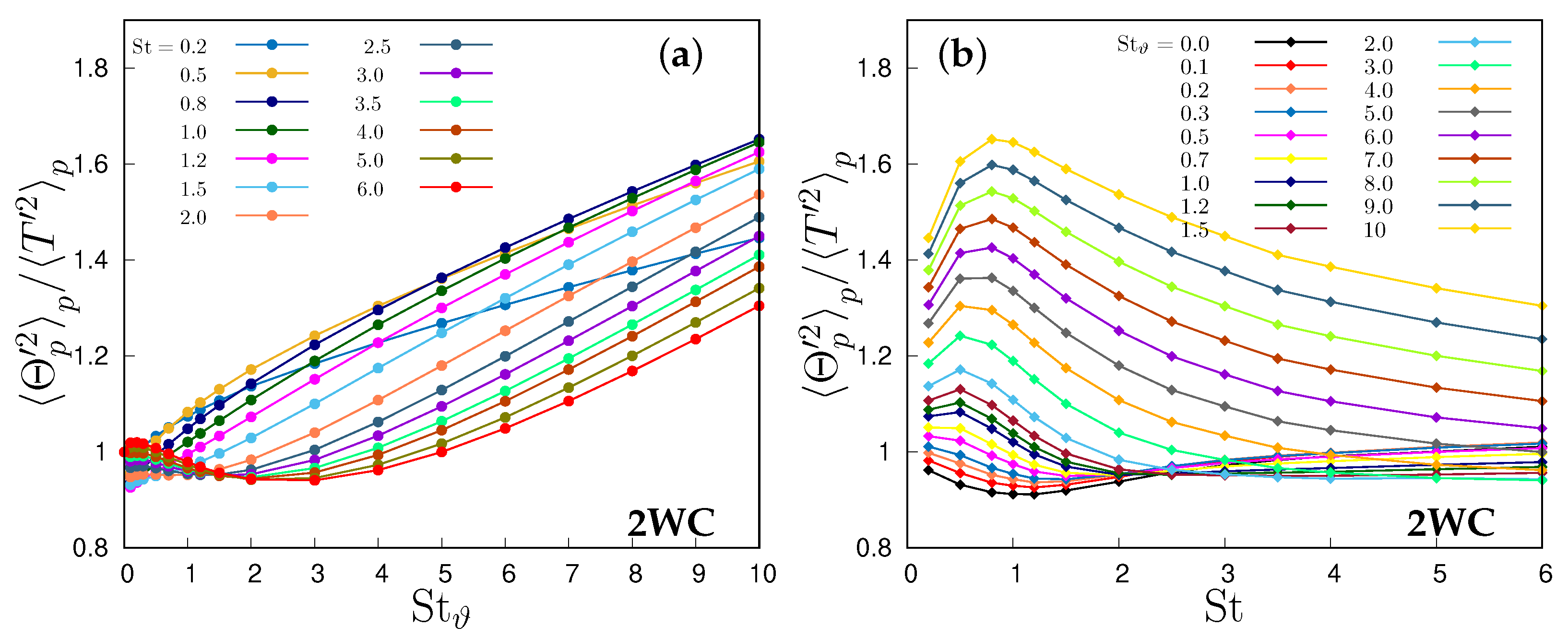
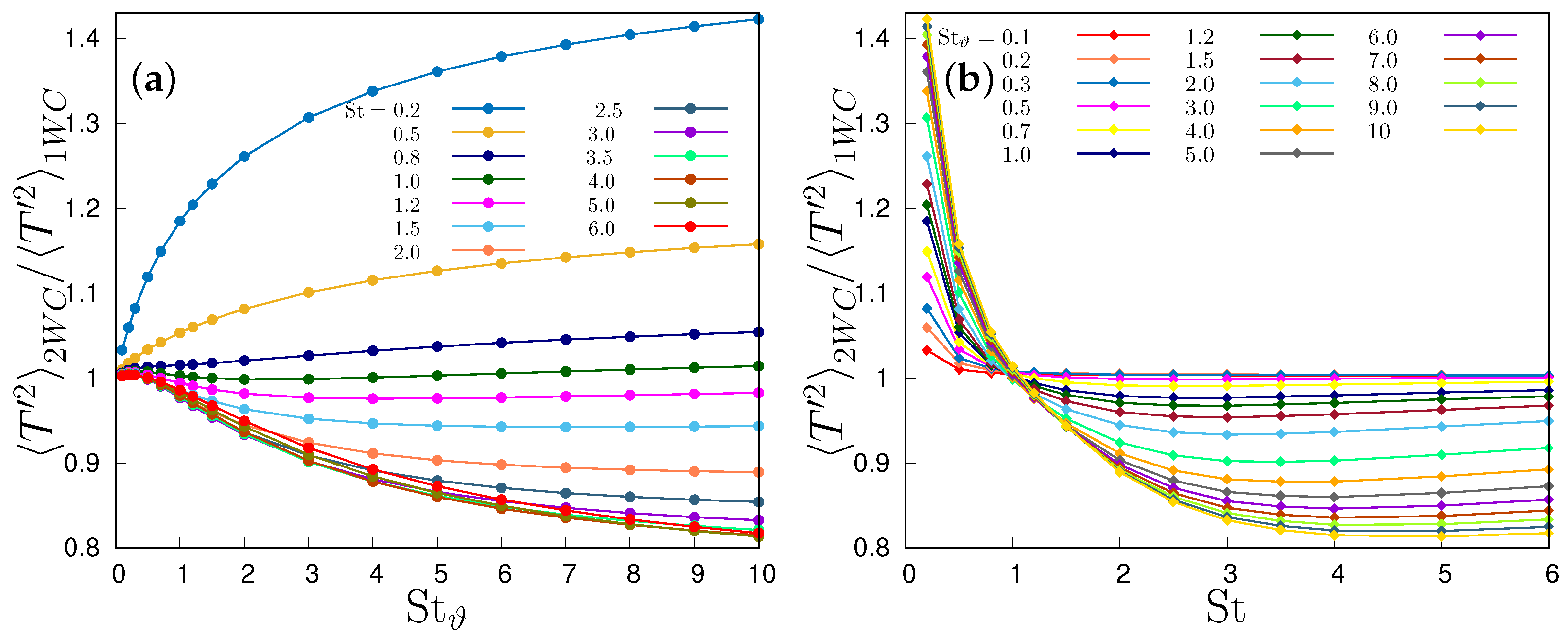
In the two-way coupling case (Figure 4), the growth with the thermal Stokes number is much faster, because the particles enhance the dissipation of fluid temperature variance [16], and this effect grows monotonically with their thermal inertia. This is essentially in agreement with our previous results [20], but in those works the ratio between particle thermal inertia and inertia is kept constant, so that an increase in inertia is associated with an increase in thermal inertia, and no independent limit with respect to each variable is possible. At very small St, when increases, the particle variance deviates from the fluid temperature variance. The effect of thermal inertia is dominant over the particle inertia in all ranges of Stokes number. Particle temperature variance is maximum for small particles with large thermal inertia (i.e., and ), as the lag between T and induced by a large allows for large particle temperatures deviations from the mean temperature of particles coming from the two homothermal regions. The minimum particle temperature variance occurs when particle relaxation time increases, , for an intermediate thermal Stokes number, as makes its variance equal to that one of the flow, and makes it increase.
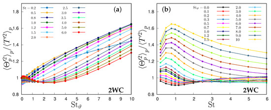
Figure 4.
Ratio between particle temperature variance to fluid temperature variance in two-way coupling simulations, (a) as a function of the thermal Stokes number and (b) as function of the Stokes number.
It should be noted that, in the two-way coupling regime, i.e., when the thermal feedback is not neglected, the interplay in Equation (15) is much more complex because T is no longer independent from so that numerator and denominator are coupled. The modulation of fluid temperature fluctuations implies that, even in the thermal ballistic limit , the ratio has no unique limit.
The effect of particle modulation of fluid fluctuations can be understood by comparing the fluid temperature variance in the one- and two- way coupling regimes, as in Figure 5, which shows the ratio of the variance between the two regimes, as a function of St and . The feedback of small particles, such that and , produces an increase in the fluid temperature variance, while larger particles with , always damp the fluid temperature fluctuations. This effect is more pronounced at large , while the modulation of the flow temperature variance by particles is almost ineffective for .
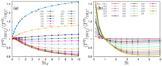
Figure 5.
Comparison between one- and two-way coupling: ratio between fluid temperature as function of (a) thermal Stokes number and (b) Stokes number.
An equation for the ratio between particle and fluid variance in a homogeneous and isotropic flow has been proposed by [34] on the basis of a Langevin equation for fluid temperature fluctuations and by [16] from the properties of the general solution of the quasi-linear equation of particle temperature and the statistics of temperature increments at very small and very large time separations. In both cases an increase in thermal inertia always led to a reduction in the ratio, as a larger inertia acts as a filter for the ambient fluctuations of T seen by the particle during its trajectory, so that
where is the time-scale of fluid temperature fluctuations sampled by the particle, proportional to the large-scale eddy turnover time and is a dimensionless coefficient, equal to 1 in [16], which in [34] depends on the “actual situation of the turbulence”, i.e., it is a fitting coefficient of the Langevin model which takes into account the effect of the finite Reynolds number on the temporal scale seen by an advected scalar. On the opposite, in the present flow configuration, a larger inertia allows more and more particles coming from one of the two homogeneous regions to keep their original temperature while they cross the thermal mixing layer, thus increasing the temperature variance inside the layer. Therefore, the presence of a temperature gradient imposed by the initial conditions, which creates a large-scale modulation of temperature on a length-scale , prevails on the small-scale effects of spatial clustering of particles at local temperature fronts located in the high-strain regions by velocity fluctuations.
3.2. Velocity–Temperature Correlation
The same argument can be used to discuss the role of inertia on the velocity–temperature correlations, which define the heat transfer across the inhomogeneous layer. Indeed, by multiplying Equations (11) and (12) and taking the conditional average, one has
which could be conveniently divided by the fluid temperature–velocity correlation to obtain
Therefore, the particle contribution to the heat flux can be decomposed in terms of the correlations between the particle derivatives and between them and the fluid velocity and temperature fluctuations.
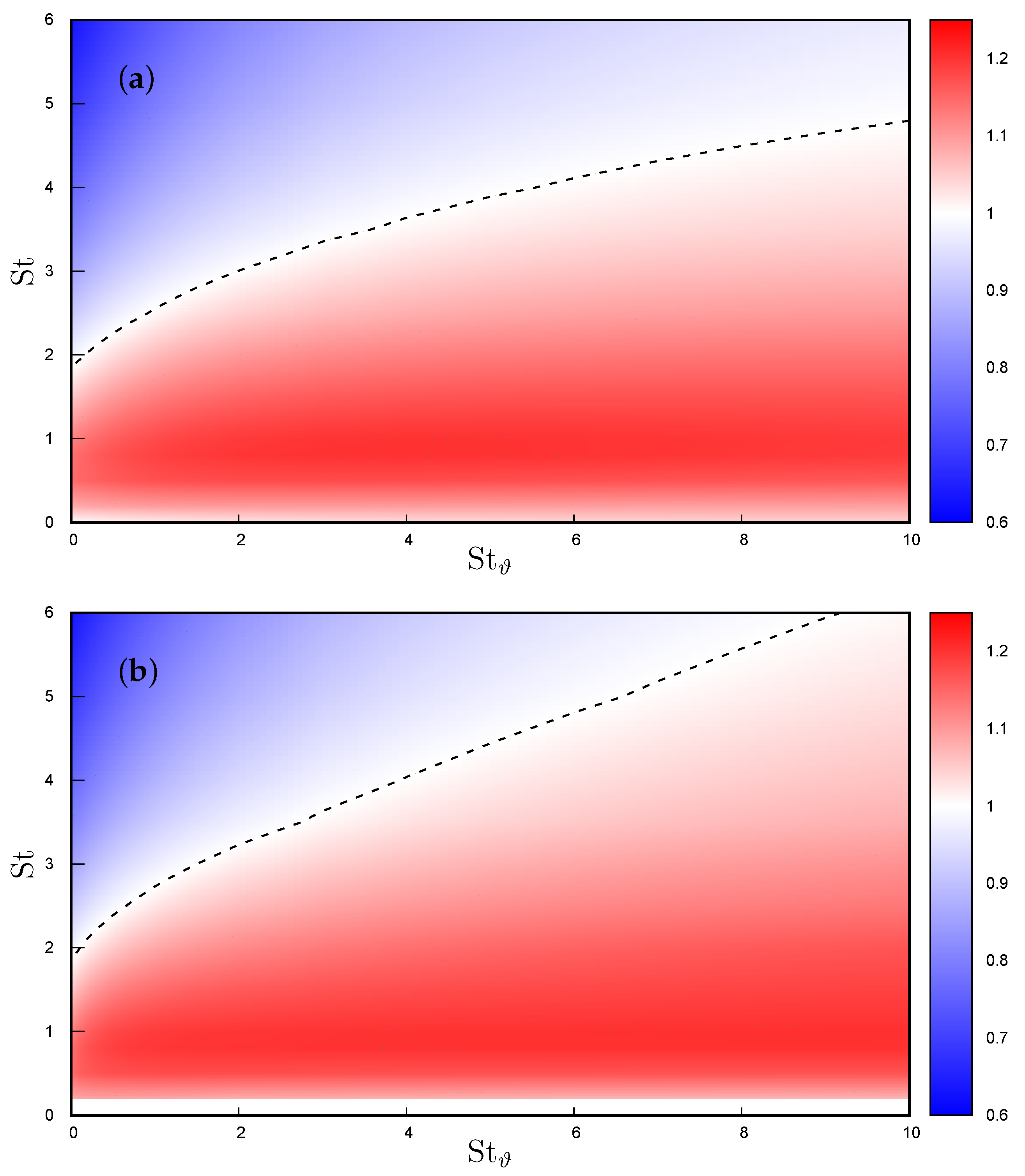
The ratio expressed in Equation (18) is directly linked to the particle contribution to the heat flux across the thermal mixing layer, as detailed in Equation (9) with respect to the convective heat flux and, as such, is one of the main objects of any modelling. The decomposition of the flux, as presented in Equation (17), allows for an understanding of how particle heat flux is affected by the particle inertia and thermal inertia, both of which modulate particle velocity and temperature time derivatives. An overview of the correlation ratio (18) is depicted in Figure 6, Figure 7 and Figure 8. Figure 6 portrays an overall view of the ratio between particle velocity–temperature correlation and fluid velocity–temperature correlation derived from 256 simulations in the one-way coupling regime and 221 simulations in the two-way coupling regimes.

Figure 6.
Normalized particle velocity–temperature correlations as function of the Stokes and thermal Stokes number: (a) one-way coupling regime, (b) two-way coupling regime. The dashed line indicates a value equal to one, where fluid and particle velocity–temperature correlations are equal.
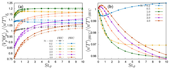
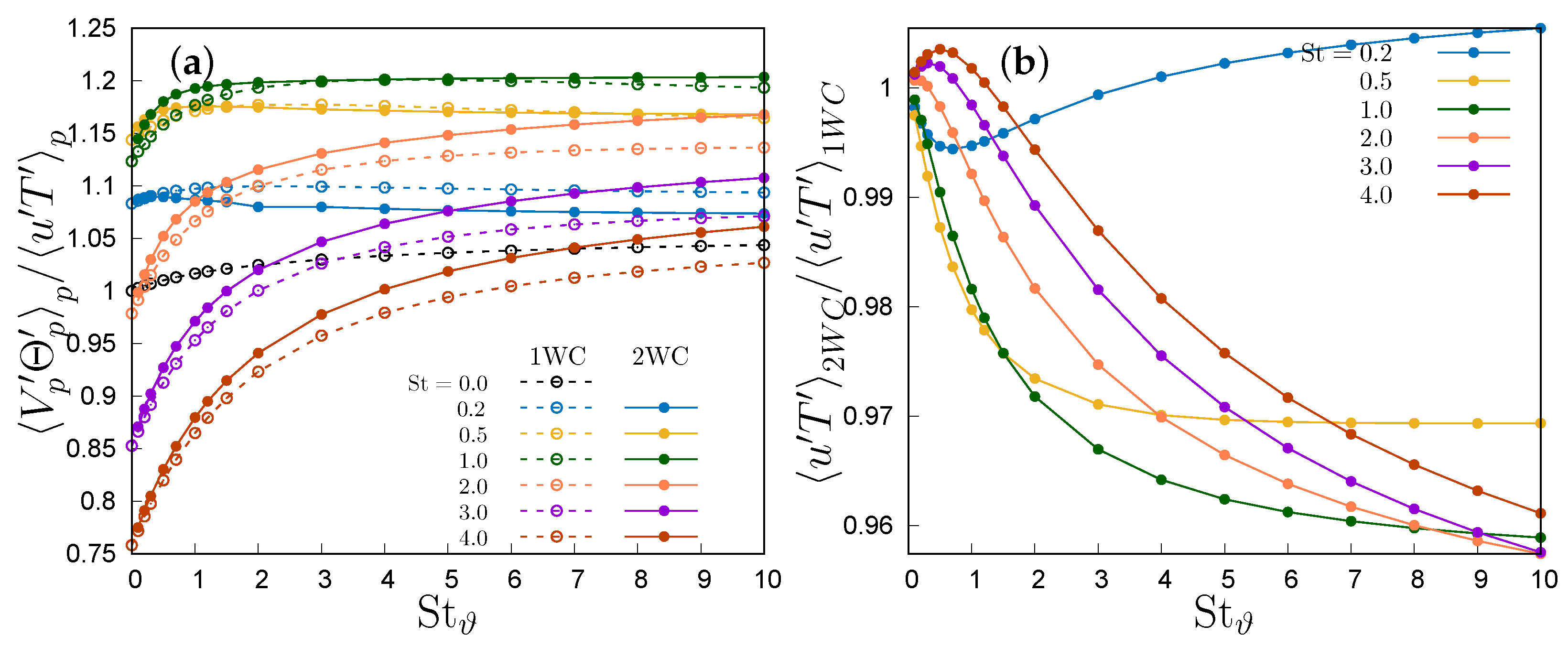
Figure 7.
(a) Normalized particle-to-fluid velocity–temperature correlation; (b) ratio between fluid velocity–temperature correlation in one- and two-way coupling regimes.
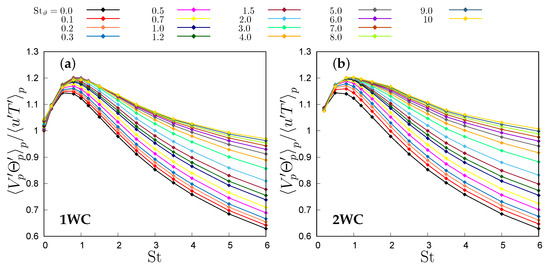
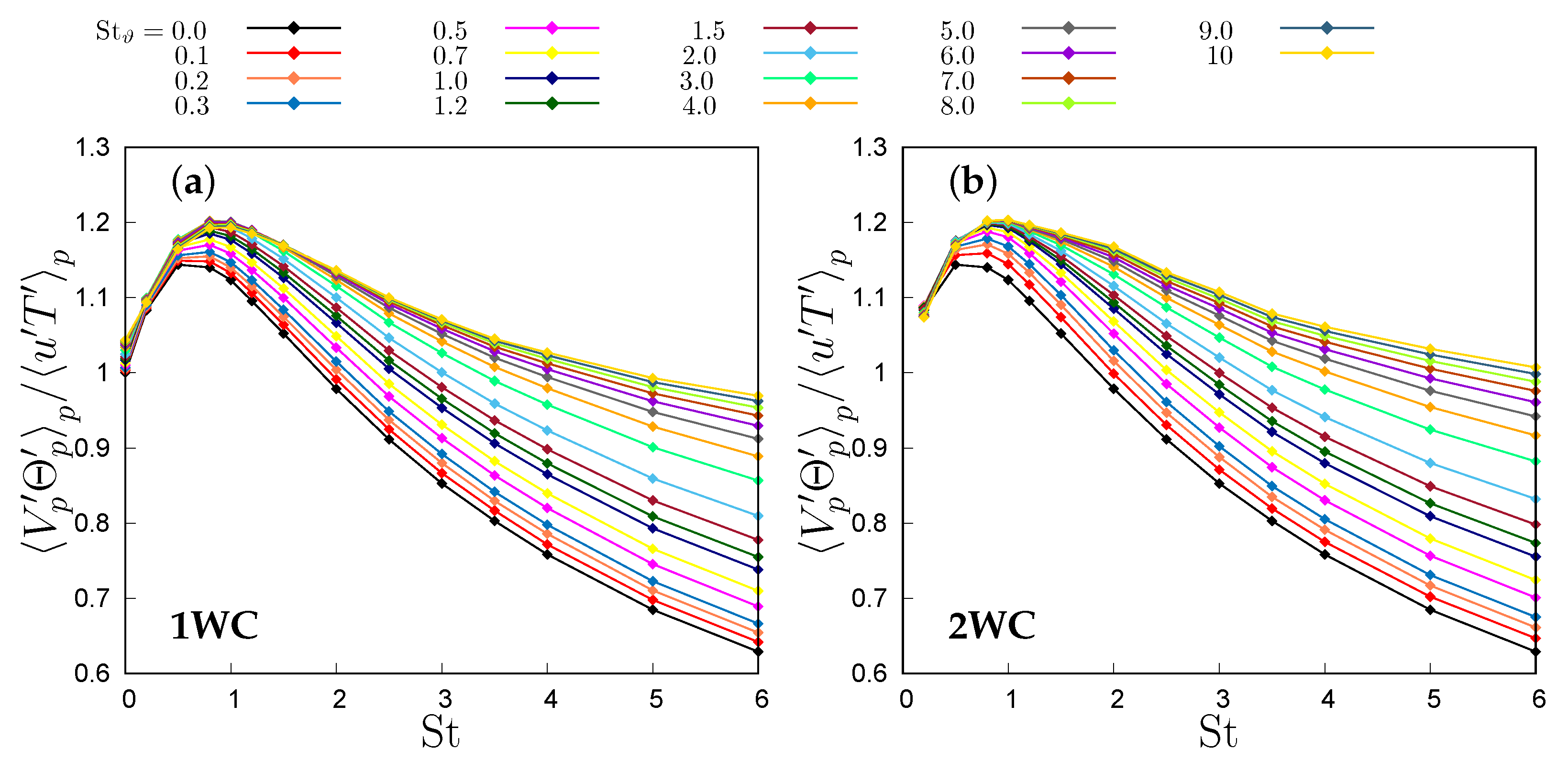
Figure 8.
Normalized particle velocity–temperature correlation as a function of the Stokes number in: (a) one-way coupling, (b) two-way coupling.
This ratio consistently increases monotonically with thermal inertia (i.e., ) at any given Stokes number, reaching an asymptotic limit dependent on the Stokes number. Particle inertia (i.e., St) makes this ratio peak when the particle relaxation time is of the same order as the Kolmogorov microscale (i.e., ), a situation where particles are expulsed from the small-scale vortex cores. This is even more clearly visible in Figure 7a, where each curve corresponds to a single Stokes number. Anyway, the limit for large Stokes number is always higher than one, that is, when the thermal Stokes number is large enough, particle velocity–temperature correlation becomes larger than the fluid–velocity correlation. By fitting the available data, the transition condition , shown by the dashed line in Figure 6, can be expressed as
with , and in the one-way coupling regime, and , and in the two-way coupling regime up to , which then tends to be linear for , with when the curve is fitted for . Any Stokes number below this threshold produces an increase in the correlation ratio, whereas for Stokes numbers larger than this threshold the ratio is below one. Thus, given , it is possible to infer that, in the ballistic limit , particle velocity and temperature consistently tend to decorrelate, irrespective of particle thermal inertia. However, in the thermal ballistic limit , a notable correlation persists, consistently surpassing the fluid correlation, especially at a Stokes number around one. This decorrelation process operates at a slower pace in the two-way coupling regime due to the particle’s thermal feedback altering fluid temperature along its trajectory. Particularly, in this regime, the modulation of fluid temperature fluctuations by particles leads to a reduction in the convective heat flux , as observed in [20]. Simulating is not possible in the two-way coupling scenario because the number of particles scales as , diverging for . Consequently, only could be represented in Figure 7. This limitation is not present in the one-way coupling regime, because particles do not influence either each other nor the fluid phase, so that their actual number is irrelevant.
The data presented in [20], where the ratio was kept fixed, correspond to a diagonal cut in Figure 6. Since
the higher the ratio of particle to fluid specific heat, the higher the overall correlation levels between particle temperature and velocity, because a lower portion of the map in Figure 6 is sampled. To keep constant the ratio between and St implies to fix the particle material while allowing the size to change so that, for any kind of particle, there is a critical Stokes number above which the correlation is lower than the fluid temperature–velocity correlation, and for increasing Stokes velocity and temperature, always decorrelate. This could not be seen in [20] because the maximum simulated Stokes number was equal to 3.
In the two-way coupling regime, particle feedback tends to increase the ratio (18), but most of the variations can be attributed to the resulting damping of fluid correlations (Figure 7b) and not to an increase in particle correlations. This damping is an effect of particle preferential concentration near the temperature fronts, as described by [16,18] in homogeneous turbulence, which smooths the fluid temperature gradients. Indeed, only for a Stokes number larger than one is there a small range of at which particle modulation of fluid fluctuations produces a slight increment in the fluid temperature–velocity correlation, which in all other situations is always reduced. This damping effect produces an overall reduction in the fluid heat flux across the thermal mixing layer except at low inertia.
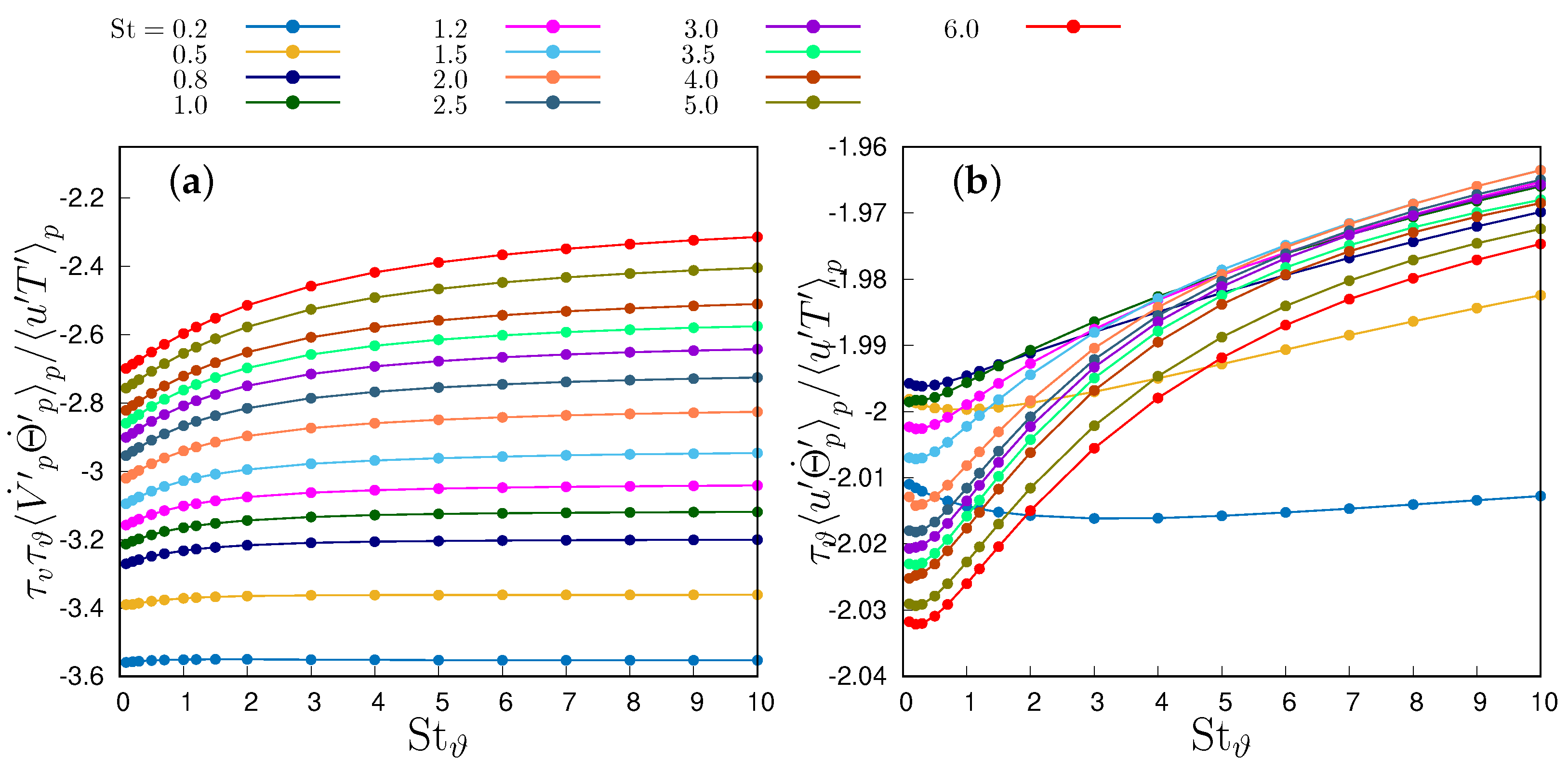
To unravel how particle inertia and thermal inertia influence the heat transfer, we examine numerical simulation data by dissecting temperature–velocity correlation using the decomposition of Equation (18). The three addends outlined in Equation (18) are shown in Figure 9 and Figure 10a for the one-way coupling case. The first term, depicted in Figure 10a, is a function of St only in the one-way coupling regime, as particle velocity and fluid temperature are independent of particle thermal inertia in that case. Its magnitude diminishes with increasing St and exhibits a negative value, akin to the second term, shown in Figure 9b. This term, , displays a mild dependence on both St and , varying no more than 2% within the investigated parameter range. Both these terms, in accordance with Equation (18)’s signs, contribute to building the particle temperature–velocity correlation, thereby elevating heat transfer. Overall, their sum decreases with the Stokes number, with a minor influence of the thermal Stokes number. On the other hand, the third addend in Equation (18), proportional to the correlation between the particle acceleration and the temperature derivative (Figure 9a), is negative due to the presence of a mean temperature gradient. This term tends to diminish the correlation, exhibiting more pronounced effects at lower Stokes numbers and diminishing with increasing St and . These variations are more gradual than the first term, thus allowing for maximal correlation around . However, it is responsible for the decorrelation at large St, given the strong dependence of the correlation between particle acceleration and temperature on St. This gradual reduction in the correlation with is far less pronounced than the reduction in the thermal time derivative variance, as shown in Figure 10b. The temperature time derivative variance increases with the Stokes number but reduces with the thermal Stokes number. It is worth noting that, based on Equation (16), the temperature derivative variance is proportional to the difference between the correlation of fluid temperature and the temperature time derivative and the correlation between the particle temperature and the temperature time derivative. In homogeneous turbulence, the presence of a smooth temperature field leads to a finite limit of the variance of for small thermal Stokes numbers [16]. Conversely, in the opposite limit, with very large thermal inertia, the acceleration integral tends to be dominated by uncorrelated temperature increments, causing its variance to decrease as [16,18]. The data illustrated in Figure 10b indicate a low thermal inertia finite limit at all simulated Stokes numbers, suggesting a smooth temperature field. Meanwhile, the behaviour in the self-similar stage in the presence of high thermal inertia demonstrates the presence of well-mixed regions within the thermal mixing layer core, approaching the asymptotic scaling found in homogeneous turbulence.

Figure 9.
(a) Normalized particle velocity and temperature derivative correlation; (b) Normalized fluid velocity–particle temperature derivative correlation.
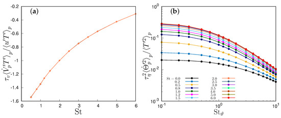
Figure 10.
(a) Normalized particle acceleration–temperature correlation; (b) normalized particle temperature derivative variance.
4. Conclusions
We have studied some aspects of the heat transfer in the simplest non-homothermal particle-laden flow, focusing on the role of inertia and thermal inertia of the suspended particles, by means of direct numerical simulations at a fixed Reynolds number. Unlikely other studies on fluid–particle thermal interaction, we have kept the Stokes and thermal Stokes number as independent parameters and explored a wide range of the parameters space, with St ranging from 0 to 6 and ranging from 0 to 10. We have determined that the Stokes number is the most relevant parameter to determine the variance of particle temperature, which, however, behaves in a different way with respect to isotropic flows. Indeed, the monotonic reduction in particle temperature variance with the Stokes number has been observed in this flow configuration only for and for large . The particle path effect responsible for the attenuation of the variance looks to be dominated by the mean gradient. We have determined the threshold of St and for which particle temperature and velocity correlate more than the fluid, which can lead to a larger contribution of particles to the overall heat flux.
We have introduced a new decomposition of second-order moments, namely the particle temperature variance and the velocity–temperature correlation, rewriting such moments in terms of correlations involving particle acceleration and thermal time derivative, to understand the properties of particle temperature fluctuations. This decomposition allows us to put into evidence the role of particle inertia and thermal inertia, since both relaxation times appear explicitly. The analysis showed the dominance of inertia over thermal inertia, because the variation of the correlation of the acceleration with the temperature determines the modulation of the particle temperature–velocity correlation, and, therefore, of the ability of particles to transfer heat between different regions. Particle thermal feedback tends to damp fluid temperature fluctuations, thus increasing the relative role of particles.
The flow configuration we have investigated, although still an idealized configuration, is the only thermally inhomogeneous particle-laden flow, apart from channel flow, which has been studied by means of direct numerical simulations. It represents one of the simplest inhomogeneous flows, with one thermally inhomogeneous direction only, and can provide useful insights into interpreting and predicting more complex flows, especially in analyzing the interrelation between particle and fluid correlations, a crucial facet in the domain of turbulence modelling. Notably, the absence of mean shear, intrinsically present in wall-bounded flows, allows us to focus on thermal effects unimpeded by the complexities inherent in velocity field inhomogeneities. Thus, it can serve as an exemplary platform for new theories and models of heat transfer in inhomogeneous turbulent particle-laden flows. In a future work a deeper understanding of this flow could be obtained by analyzing the probability density function of the fluid and particles.
Author Contributions
Conceptualization, H.R.Z.P. and M.I.; methodology, H.R.Z.P. and M.I.; software, H.R.Z.P. and M.I.; formal analysis, H.R.Z.P. and M.I.; investigation, H.R.Z.P. and M.I.; writing—original draft preparation, H.R.Z.P. and M.I.; writing—review and editing, H.R.Z.P. and M.I.; visualization, H.R.Z.P. and M.I.; supervision, M.I. All authors have read and agreed to the published version of the manuscript.
Funding
This research received no external funding.
Data Availability Statement
Data are available from the authors upon reasonable request. Due to the article does not contain table with the data of the figures.
Acknowledgments
The authors acknowledge the CINECA award IsB26_DroMiLa, HP10BU46TS, under the ISCRA initiative, for the availability of high performance computing resources and support. Additional computational resources provided by hpc@polito (http://www.hpc.polito.it) (accessed on 15 January 2024) are also gratefully acknowledged.
Conflicts of Interest
The authors declare no conflict of interest.
Appendix A
By using the normalization defined in (7), having chosen , the dimensionless form of the governing Equations (1)–(3) for the carrier flow is
where is the Reynolds number, is the Prandtl number. This equations are solved in a domain with periodic boundary conditions on , , . Equation (4) becomes, in dimensionless form,
where the dimensionless particle relaxation times are given by
Finally, the dimensionless particle feedback term can be expressed as
where is the particle to fluid heat capacity ratio. A deterministic body force , linear function of the velocity, is used in Equation (A2) to keep the velocity field statistically steady by injecting energy in a single wavenumber (see also [16,20] for further details about the forcing). In dimensionless form its representation in the Fourier space is given by
The dimensionless formulation of the physical model of this section is the one actually discretized by the numerical code.
References
- Taylor, G.I. Diffusion by Continuous Movements. Proc. Lond. Math. Soc. 1922, 2, 196–212. [Google Scholar] [CrossRef]
- Kraichnan, R.H. Anomalous scaling of a randomly advected passive scalar. Phys. Rev. Lett. 1994, 72, 1016–1019. [Google Scholar] [CrossRef] [PubMed]
- Zheng, X.; Wang, G.; Zhu, W. Experimental study on the effects of particle–wall interactions on VLSM in sand-laden flows. J. Fluid Mech. 2021, 914, A35. [Google Scholar] [CrossRef]
- Liu, H.; Feng, Y.; Zheng, X. Experimental investigation of the effects of particle near-wall motions on turbulence statistics in particle-laden flows. J. Fluid Mech. 2022, 943, A8. [Google Scholar] [CrossRef]
- Lewis, E.W.; Lau, T.C.W.; Sun, Z.; Alwahabi, Z.T.; Nathan, G.J. Insights from a new method providing single-shot, planar measurement of gas-phase temperature in particle-laden flows under high-flux radiation. Exp. Fluids 2021, 62, 80. [Google Scholar] [CrossRef]
- Banko, A.J.; Villafañe, L.; Kim, J.H.; Eaton, J.K. Temperature statistics in a radiatively heated particle-laden turbulent square duct flow. Int. J. Heat Fluid Flow 2020, 84, 108618. [Google Scholar] [CrossRef]
- Reeks, M.W. On a kinetic equation for the transport of particles in turbulent flows. Phys. Fluids A Fluid Dyn. 1991, 3, 446–456. [Google Scholar] [CrossRef]
- Pandya, R.; Mashayek, F. Non-isothermal dispersed phase of particles in turbulent flow. J. Fluid Mech. 2003, 475, 205–245. [Google Scholar] [CrossRef]
- Zaichik, L.I.; Alipchenkov, V.M.; Avetissian, A.R. A Statistical model for predicting the heat transfer of solid particles in turbulent flows. Flow Turbul. Combust 2011, 86, 497–518. [Google Scholar] [CrossRef]
- Zonta, F.; Marchioli, C.; Soldati, A. Direct numerical simulation of turbulent heat transfer modulation in micro-dispersed channel flow. Acta Mech. 2008, 195, 305–326. [Google Scholar] [CrossRef]
- Kuerten, J.G.M.; van der Geld, C.W.M.; Geurts, B.J. Turbulence modification and heat transfer enhancement by inertial particles in turbulent channel flow. Phys. Fluids 2011, 23, 123301. [Google Scholar] [CrossRef]
- Nakhaei, M.; Lessani, B. Effects of solid inertial particles on the velocity and temperature statistics of wall bounded turbulent flow. Int. J. Heat Mass Transf. 2017, 106, 1014–1024. [Google Scholar] [CrossRef]
- Lessani, B.; Nakhaei, M. Large-eddy simulation of particle-laden turbulent flow with heat transfer. Int. J. Heat Mass Transf. 2013, 67, 974–983. [Google Scholar] [CrossRef]
- Pouransari, H.; Mani, A. Effects of Preferential Concentration on Heat Transfer in Particle-Based Solar Receivers. J. Sol. Energy Eng. 2016, 139, 021008. [Google Scholar] [CrossRef]
- Pouransari, H.; Mani, A. Particle-to-fluid heat transfer in particle-laden turbulence. Phys. Rev. Fluids 2018, 3, 074304. [Google Scholar] [CrossRef]
- Carbone, M.; Bragg, A.D.; Iovieno, M. Multiscale fluid–particle thermal interaction in isotropic turbulence. J. Fluid Mech. 2019, 881, 679–721. [Google Scholar] [CrossRef]
- Saito, I.; Watanabe, T.; Gotoh, T. A new time scale for turbulence modulation by particles. J. Fluid Mech. 2019, 880, R6. [Google Scholar] [CrossRef]
- Béc, J.; Homann, H.; Krstulovic, G. Clustering, Fronts, and Heat Transfer in Turbulent Suspensions of Heavy Particles. Phys. Rev. Lett. 2014, 112, 234503. [Google Scholar] [CrossRef]
- Zandi Pour, H.R.; Iovieno, M. Heat transfer enhancement by suspended particles in a turbulent shearless flow. In Proceedings of the 33rd Congress of the International Council of the Aeronautical Sciences, ICAS 2022, Stockholm, Sweden, 4–9 September 2022; Volume 4, pp. 2452–2463. [Google Scholar]
- Zandi Pour, H.R.; Iovieno, M. Heat Transfer in a Non-Isothermal Collisionless Turbulent Particle-Laden Flow. Fluids 2022, 7, 345. [Google Scholar] [CrossRef]
- Zandi Pour, H.R.; Iovieno, M. The Impact of Collisions on Heat Transfer in a Particle-Laden Shearless Turbulent Flow. J. Fluid Flow Heat Mass Transf. 2023, 10, 131–140. [Google Scholar] [CrossRef]
- Zandi Pour, H.R.; Iovieno, M. On the Heat Transfer in Particle-laden Turbulent Flows: The Effect of Collision in an Anisothermal Regime. In Proceedings of the 9th World Congress on Mechanical, Chemical, and Material Engineering, London, UK, 6–8 August 2023. [Google Scholar] [CrossRef]
- Zamansky, R. Acceleration scaling and stochastic dynamics of a fluid particle in turbulence. Phys. Rev. Fluids 2022, 7, 084608. [Google Scholar] [CrossRef]
- Buaria, D.; Sreenivasan, K.R. Lagrangian acceleration and its Eulerian decompositions in fully developed turbulence. Phys. Rev. Fluids 2023, 8, L032601. [Google Scholar] [CrossRef]
- Götzfried, P.; Kumar, B.; Shaw, R.A.; Schumacher, J. Droplet dynamics and fine-scale structure in a shearless turbulent mixing layer with phase changes. J. Fluid Mech. 2017, 814, 452–483. [Google Scholar] [CrossRef]
- Bhowmick, T.; Iovieno, M. Direct numerical simulation of a warm cloud top model interface: Impact of the transient mixing on different droplet population. Fluids 2019, 4, 144. [Google Scholar] [CrossRef]
- Gatignol, R. Faxen formulae for a rigid particle in an unsteady non-uniform stokes flow. J. Mec. Theor. Appl. 1983, 2, 143–160. [Google Scholar]
- Maxey, M.R.; Riley, J.J. Equation of motion for a small rigid sphere in a nonuniform flow. Phys. Fluids 1983, 26, 883–889. [Google Scholar] [CrossRef]
- Canuto, C.; Hussaini, M.Y.; Quarteroni, A.; ZangHawking, T.A. Spectral Methods in Fluid Dynamics; Springer: Berlin/Heidelberg, Germany, 1988. [Google Scholar] [CrossRef]
- Carbone, M.; Iovieno, M. Application of the Non-Uniform Fast Fourier Transform to the Direct Numerical Simulation of two-way coupled turbulent flows. WIT Trans. Eng. Sci. 2018, 120, 237–248. [Google Scholar] [CrossRef]
- Carbone, M.; Iovieno, M. Accurate direct numerical simulation of two-way coupled particle-laden flows through the nonuniform Fast Fourier Transform. Int. J. Saf. Sec. Eng. 2020, 10, 191–200. [Google Scholar] [CrossRef]
- Iovieno, M.; Di Savino, S.; Gallana, L.; Tordella, D. Mixing of a passive scalar across a thin shearless layer: Concentration of intermittency on the sides of the turbulent interface. J. Turbul. 2014, 15, 311–334. [Google Scholar] [CrossRef]
- Mydlarski, L.; Warhaft, Z. Passive scalar statistics in high Péclet number grid turbulence. J. Fluid Mech. 1998, 358, 135–175. [Google Scholar] [CrossRef]
- Saito, I.; Watanabe, T.; Gotoh, T. Modulation of fluid temperature fluctuations by particles in turbulence. J. Fluid Mech. 2022, 931, A6. [Google Scholar] [CrossRef]

Disclaimer/Publisher’s Note: The statements, opinions and data contained in all publications are solely those of the individual author(s) and contributor(s) and not of MDPI and/or the editor(s). MDPI and/or the editor(s) disclaim responsibility for any injury to people or property resulting from any ideas, methods, instructions or products referred to in the content. |
© 2024 by the authors. Licensee MDPI, Basel, Switzerland. This article is an open access article distributed under the terms and conditions of the Creative Commons Attribution (CC BY) license (https://creativecommons.org/licenses/by/4.0/).