Abstract
This work studies how the sliding-gate valve (SGV) modifies the features and the dynamic behavior of the outlet jets for flat-bottom and well-bottom bifurcated submerged entry nozzles (SENs) used in continuous casting machines. Three conditions for the SGV were studied: no obstruction, moderate obstruction, and severe obstruction. The experimental study used a scaled model, employing cold water as the working fluid. A high-frequency analysis of the flow inside the SEN’s bore arriving at the outlet ports was performed by employing the particle image velocimetry (PIV) technique. Low-frequency measurements of the volumetric flow at the exit port were obtained by splitting the exit jet into four quadrants and employing digital flowmeters. It was observed that reducing the SGV clearance increases the turbulence of the flow inside the SEN bore, but the flow displays ordered rather than erratic fluctuations. Flowmeter measurements showed that, regardless of the level of obstruction in the SGV, the outlet jets on flat-bottom and the well-bottom SENs have dynamic behaviors and features with significant differences. This finding is relevant because the flow distribution inside the outlet ports is directly related to the jet’s wideness, affecting the recirculation pattern inside the mold and, therefore, the quality of the finished steel slab.
1. Introduction
Steel is a crucial material in the circular economy, a model of production and consumption that aims to minimize waste and promote the sustainable use of natural resources [1]. Recent works estimate that the global steel demand in 2050 will range from 2300 to 3000 million tons annually [2,3,4]. This colossal demand presents steelmakers with an enormous challenge, given that steel production generates around 7% of all CO2 emissions [5]. Continuous casting is the world’s predominant method for producing steel slabs [6,7]. Today, the industry uses at least three different types of continuous casting: conventional continuous casting (CCC), endless strip production (ESP), and thin slab caster (TSC). CCC remains the preferred method for producing the highest-quality steel sheet products [8]. In the CCC process, the quality of the finished steel slab depends on numerous factors which are intimately related to the fluid flow pattern inside the mold [9,10]. In turn, the hydrodynamic pattern within the mold depends strongly on the characteristics of the jets emerging from the exit ports on the submerged entry nozzle (SEN), whose design varies widely. The cylindrical-like external geometry of the SEN is the most common shape in CCC machines [11,12]. Typically, the shape of the SEN bore is also cylindrical [13]. The features of the SEN that have been employed to modify the hydrodynamic behavior inside the mold include the height of the inner bottom wall [13,14,15], and the number [16] and shape of the exit ports [17].
Besides modifying the geometric features of the SEN, an external device, the electromagnetic brake, has also been employed to impose a prescribed fluid flow pattern inside the mold [18,19,20]. Although this device has produced favorable results, recent works have shown that the magnetic field’s features must be tuned carefully. Specifically, an undesirable hydrodynamic behavior inside the mold is obtained when the magnetic field is set incorrectly [21,22,23].
Finally, the device that controls the flow of the liquid steel from the tundish to the mold is an element that must be included in the process analysis [11,24,25,26]. Several investigations studying these devices’ effects on the characteristics of the jets that emerge from the SEN are reported in the literature [25,27]. The results are phenomenologically consistent but have a level of uncertainty that is difficult to delimit. In addition, these investigations involve a complex methodology and expensive equipment [24]. Using numerical simulations, Bai and Thomas explained the features of SEN exit jets by splitting each of them into two parts: the upward and the downward jets [28]. Bai and Thomas report that, although the upward jet occupied around 30% of the exit port area, the volumetric flow fraction corresponding to this jet is considerably less than 30%. However, to the authors’ knowledge, there are no works reported in the literature that, through physical simulations, fully corroborate or refute the assertions of Bai and Thomas.
Numerous works have employed numerical and physical simulations to design the shape of an SEN to enhance the steel quality. Based on similarity criteria, the hydrodynamic behavior of an actual steel CCC can be reproduced in a scaled model using cold water as the working fluid if the dimensions and operating conditions are set correctly [29]. This work is devoted to experimentally studying, in a scaled cold-water model, how the sliding-gate valve (SGV) modifies the hydrodynamic pattern inside the SEN and the characteristics of the jets emerging from it. The study included two variants of the bifurcated SEN, one with a flat bottom and another with a pool at the bottom. In addition, three “positions” or conditions of the SGV were studied: one where there is no flow obstruction, one with moderate obstruction, and another with severe obstruction. Based mainly on numerical simulations, previous works stated that the uneven distribution of the liquid flow across the SEN outlet largely determines the features of the exit jet [27,28]. The present work conducted experimental tests employing a modified SEN to divide each outlet into four quadrants and measure the volumetric flow crossing each. Our work confirms that the flow at the SEN outlet is distributed unevenly, and this distribution depends on the shape of the bottom of the SEN and the SGV clearance.
This work is organized as follows. The operating conditions of the scaled model of the SEN and its relationship with an actual CCC are presented in Section 2. The dimensions and the geometric features of the six SEN configurations studied in this work are also described and discussed in this section. Section 3 presents and analyzes the high-frequency, transient behavior of the fluid velocity field inside the SEN’s bore in a zone above the exit ports obtained with the particle image velocimetry technique (PIV). The low-frequency, transient behavior of the SEN outlet jets is presented and analyzed in Section 4. In this case, each jet was divided into four quarters, and the volumetric flow that emerged from each quarter was measured using digital flowmeters. These temporal signals were subsequently analyzed. This section also discusses the adjustments made to the SEN to couple it with the flowmeters, and through numerical simulations, it is shown that these adjustments do not modify the fluid flow pattern inside the SEN. Finally, Section 5 presents some concluding remarks of this work and discusses its implications for actual CCC.
2. The CCC Process and the SEN Designs Studied in This Work
The molten steel with the specified composition is transported from the secondary refinement facility to the continuous casting section inside a ladle. There, the steel is discharged into the tundish, a container that distributes the molten steel into several casting lines. The molten steel is poured into the solidification mold through the SEN. The left-hand panel in Figure 1 shows a schematic of the casting section in a CCC machine for producing steel slabs. The solidification of the molten steel is initiated inside the mold, which is a water-cooled copper shell. The secondary cooling section is just below the mold, where, besides the steel slab being sprayed with cold water, the steel slab is pulled by withdrawal rollers. Typically, the mold width ranges from to . When the slab width is above , it is considered a wide slab, and it is considered an ultra-wide slab when the width is close to [30]. The thickness of the mold ranges from to , and its length is around [31]. In CCC, the casting speed is the velocity at which the semi-solidified slab is drawn from the mold. Nowadays, most continuous casters work at speeds between and [7].
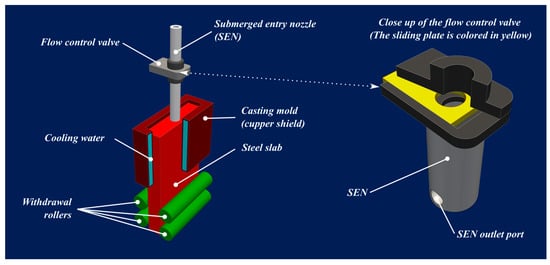
Figure 1.
Schematic description of the casting section of a continuous casting machine for making steel slabs.
In actual CCC machines, each steelmaking company uses the SEN design that best meets its requirements, so its geometric characteristics can change [32,33]. The main design parameters for the SENs are the number, the shape, and the vertical tilt of the exit ports. Regarding the number, the preferred configuration is the bifurcated one with an SEN with two exit ports near the pipe’s end. Each port is located on opposite sides of the SEN, so the exit ports’ axis is perpendicular to the SEN’s longitudinal axis. To minimize defects generated by an asymmetric fluid flow pattern inside the mold, the axis of the outlet ports of a bifurcated SEN must be parallel to the mold’s wide walls. The most common shapes used for the exit ports are rectangular, circular, and oval [34]. In addition, the SEN could have outlet ports with a vertical tilt upwards, horizontally, or downwards [35,36,37]. In this work, the SEN designs have two outlet ports with a circular shape, and their vertical tilt is downward.
The flow entering the mold from the tundish is usually controlled by an SGV or a stopper rod (SR) [25,26,38,39,40]. However, this work will only consider the SGV as the flow-control device. The right-hand panel in Figure 1 shows a close-up of the SGV coupled with a bifurcated SEN. The SGV has an orifice in a plate that controls the steel’s flow rate. The volumetric flow descending through the SEN depends on the height of the steel inside the tundish, which varies constantly. At the beginning of the cast, the tundish is filled to its maximum capacity, and the height of the molten steel decreases as the casting progresses until the tundish is filled again. So, to maintain a constant delivery of molten steel to the mold, the SGV plate’s clearance is narrow at the beginning of the cast, increasing as the molten steel’s height into the tundish decreases. An analysis of the transient reduction in the SGV plate’s clearance is beyond the scope of the present work. Instead, three conditions of the SGV are studied: no flow obstruction, moderate flow obstruction, and severe flow obstruction.
Figure 2 shows three ways of coupling the SGV with the SEN. The coupling is named after the angle formed between the axis of the sliding plate, colored in yellow, and the SEN outlet ports: , , and . Several works show that the coupling induces less asymmetry in the fluid flow pattern inside the mold [27]. So, in all the SEN designs studied in this work, the axes of the sliding plate and the SEN outlet ports will be perpendicular to each other.
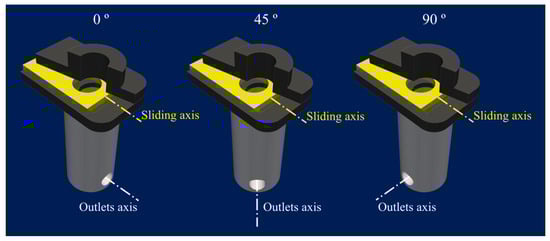
Figure 2.
Typical arrangements of the tundish sliding-gate valve with respect to the axes of the exit ports of a bifurcated SEN.
Another design parameter for a bifurcated SEN is the height of the inner bottom wall relative to the height of outlet ports’ inner lower edges. When the heights of the wall and the edges coincide, the design is labeled as a Flat-Bottom (FB) SEN. Otherwise, a pool or well emerges inside the SEN when the bottom wall height is below the ports’ lower edges. Therefore, the design is called a Well-Bottom (WB) SEN. Figure 3 shows a conventional bifurcated SEN and the customized designs employed in this work. The customization relies on reducing the thickness of the walls to obtain SENs with extra-thin walls, so the sections colored in dark grey are removed. Therefore, the SENs employed in this work are composed only of the sections colored in light grey.
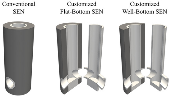
Figure 3.
Conventional SEN and customized FB and WB SEN designs.
The kinematic viscosity of water at 25 °C and molten steel at 1550 °C are and , respectively. Given that the kinematic viscosity of these two fluids is close enough, in 1972, Szekely and Yadoya showed that the hydrodynamic behavior inside a scaled model using water is similar to a CCC, ensuring the Froude number in both models is the same and that the liquid velocity in the scaled model is set correctly [29]. A scaled model ensuring thermal similarity with a CCC requires fulfilling other requirements. However, this work is restricted to studying the hydrodynamic behavior inside the SEN. Based on the previous discussion, the Froude similarity criterion between an actual CCC and the scaled model must be satisfied to specify the SEN dimensions and the operating conditions.
The left-hand panel in Figure 4 shows the dimensions of the customized SENs studied in this work based on a scale factor of . All the SENs have a bore diameter, , of ; the outlet port inner diameter, , is ; and their vertical tilt is downwards. This panel also shows the width of the plate’s clearance for the moderatep and severe-SGV-obstruction conditions, which are 15 and 10 mm, respectively. These obstruction degrees agree with those employed in actual CCC machines. The obstruction plate, shown in blue in this figure, is above the outlet ports’ upper edge. This positioning ensures that the plate’s distance to the outlet ports is at least ten times the SEN’s bore’s diameter, D.
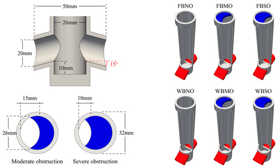
Figure 4.
The left-hand panel shows the dimensions of SEN and the SGV clearance. The right-hand panel provides a 3D view of the six SEN configurations studied in this work.
The right-hand panel in Figure 4 depicts the six customized SEN designs studied in this work: flat-bottom with no obstruction (FBNO), flat-bottom with moderate obstruction (FBMO), flat-bottom with severe obstruction (FBSO), well-bottom with no obstruction (WBNO), well-bottom with moderate obstruction (WBMO), and well-bottom with severe obstruction (WBSO). The SEN’s central long body was made with a Plexiglass pipe 3 mm in thickness. For the experiments presented in Section 3, the outlet ports, colored in red in Figure 4, were also made with Plexiglass pipes 3 mm in thickness. For convenience, in the experiments presented in Section 4, the SEN outlet ports were manufactured on a printer with PLA filament, and their thicknesses were also .
Regarding the operating conditions, all the experiments were conducted using the same water volumetric flow, . Recalling that the scale factor is for an actual mold with a width of and a thickness of , the casting speed in the cold-water scaled model with this volumetric flow is . The measurements used in this analysis begin 30 s after the pump is turned on.
3. Transient Behavior of the Fluid Velocities Field inside the SEN’s Bore
The transient behavior inside the SEN’s bore is analyzed by calculating the fluid velocity field using the particle image velocimetry technique (PIV). The analysis is restricted to a central plane above but near the SEN’s bottom zone. Figure 5 shows a schematic representation of the experimental rig employed for the PIV test, and a photo of the SEN used in these experiments. To allow us to see inside the SEN’s bottom zone, at least partially, the camera’s sensor and the laser sheet were not parallel. Notice that the entire SEN is made from Plexiglass pipes. The lower end of the central tube is closed using the stoppers (black), also shown in the figure. The stoppers’ heights are different, allowing for both the FB and the WB SEN designs to be generated. After several attempts, the best video recordings were obtained when the SEN discharged the water jets directly into the air instead of submerging the SEN into a transparent receptacle filled with water. Therefore, two gadgets made of white PVC plumbing were attached to each outlet port, directing the water jets downward and avoiding excessive splashing. These gadgets are also shown in Figure 5. The device used to recreate the sliding plate under the severe obstruction condition is also shown in Figure 5. This device was manufactured with a printer with PLA filament. The other device used to recreate the moderate obstruction condition is similar to this one.
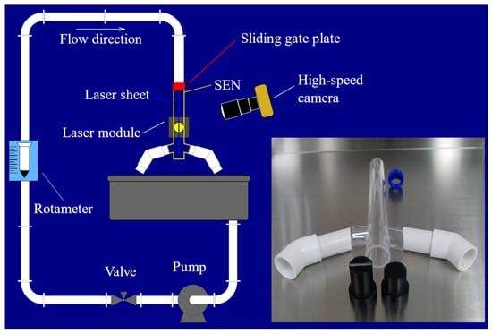
Figure 5.
Schematic representation of the experimental rig employed for the PIV test. The inset shows a picture of the customized SEN and its associated devices.
The experimental tests reported and analyzed in this section were recorded using a monochromatic 9501AZ High-Speed Camera from AZ-Instruments Corp. (Taichung City, Taiwan), using a , , , CS lens. Hollow glass spheres from Dantec Dynamics A/S (Skovlunde, Denmark), with diameters of , were used as seeding particles to trace the fluid flow pattern. The SEN bore was illuminated using a , laser module, which generated a thick lighting sheet. All the experimental tests were recorded at frames per second, with a image resolution. So, the elapsed time between each pair of consecutive images is . This time gap is small enough because all the liquid velocities are expected to be below .
The left panel in Figure 6 shows a pair of consecutive images for the FBNO configuration to exemplify the recording results used for PIV analysis. Notice that the plane under study is perpendicular to the SEN outlet port’s axis. The plane to be analyzed starts from the SEN’s bottom zone and extends above the level of the exit ports to a height around twice the diameter of the SEN bore. The right panel in Figure 6 shows the flow pattern of the liquid in a zone just below the SVG. This image shows the path of reflective particles illuminated by a laser sheet. The particles’ path becomes visible by setting the camera’s exposure time high enough. The SGV creates two zones below it, the main flow and the recirculation zones, which are enclosed in red- and blue-colored rectangles, respectively. The importance of this flow separation will be highlighted below.
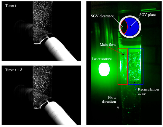
Figure 6.
Left panel: A pair of consecutive images inside the SEN bore for the FBNO configuration. The image on the top was captured 1.2 ms after the one on the bottom. Right panel: Image showing the flow pattern inside the zone just below the SVG. The main flow and the recirculation zones are enclosed in red and blue colored rectangles, respectively.
For the sake of space, the transient analysis of the velocities field inside the SEN bore will only be shown for the no-obstruction and severe-obstruction conditions. However, video files for the six SEN configurations are provided as Supplementary Materials. Figure 7 and Figure 8 display the velocity fields for the FB and WB designs, respectively. Both figures have the same structure: The upper panels belong to the no-obstruction condition, whereas the lower panels were reported in the severe-obstruction condition. The flow patterns sketched on the right-hand side of Figure 7 and Figure 8 were made based on the behavior observed in the high-speed recordings and the results of previous works reported in the literature.
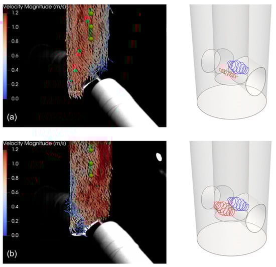
Figure 7.
Left-hand panels: fluid velocity field for the FB design with no obstruction (a), and severe obstruction (b). The green dots are the measurements points. Right-hand panels: Red and blue lines outline the vortexes inside the SEN.
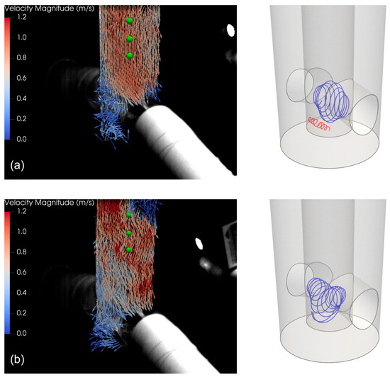
Figure 8.
Left-hand panels: fluid velocity field for the WB design with no obstruction (a), and severe obstruction (b). The green dots are the measurements points. Right-hand panels: Red and blue lines outlinethe vortexes inside the SEN.
The upper panels in Figure 7 and Figure 8 show that, for the no-obstruction condition and regardless of the SEN bottom shape, the liquid’s flow pattern above the outlet ports zone resembles a fully developed turbulent flow. This flow pattern is distorted near the upper edges of the outlet ports. On the contrary, and as expected, the lower panels in Figure 7 and Figure 8 show that the obstruction increases the intensity of the turbulence in the flow inside the SEN bore, but the flow displays ordered rather than erratic fluctuations. It can be noticed, in Figure 7 and Figure 8, that the fluid-flow pattern is distorted differently when the liquid reaches the beginning of the outlet ports in the no-obstruction (panel a) and severe-obstruction conditions (panel b). We assume that this difference reflects a change in the flow pattern in the SEN’s bottom zone.
For the FB design (Figure 7), it is well known that two counter-rotating vortexes characterize the flow pattern at the bottom of the SEN, and many works report that their sizes and intensities are the same [41,42]. However, recent studies have shown that the intensity of the vortexes can differ, and the small, weaker vortex can even disappear periodically. Precisely this behavior was observed for the no-obstruction condition [43,44,45]. On the other hand, for the severe-obstruction condition, the permanent presence of two vortexes with almost the same sizes and intensities was observed.
Concerning the WB design, several works have reported that the flow pattern at the bottom of the SEN is characterized by two counter-rotating vortexes, whose sizes and intensities differ enormously [45,46]. The biggest and strongest vortex occupies a significant fraction of the volume of the pool at the bottom of the SEN and extends to a height close to three-quarters of the height of the exit ports. On the contrary, the smallest and weaker vortex is inside the liquid pool, close to its bottom wall. This behavior coincides with that observed in experiments for the no-obstruction condition. However, for the severe-obstruction condition, the intensity of the biggest vortex increases, is pushed downwards, and sinks into the pool, occupying its volume almost entirely, and causing the weaker vortex to disappear. Additionally, it can be noticed that there is an increase in spreading in the stagnation zone above the ports and below the SGV plate clearance.
The analysis of the fluid transient velocity fields for each experiment was carried out using a set of pairs of consecutive images. However, only the results at the locations marked with green spheres in Figure 7 and Figure 8 are reported and analyzed, which were obtained from nodes of VTK files generated by PIVlab v2.62. Each location is named after its height: upper, middle, and lower. Figure 9 shows the evolution of the fluid velocity magnitude, , over time for the four configurations and at the three locations. Figure 10 shows the evolution of the velocity vector vertical tilt, , over time. By observing the curves in these figures, the change in behavior under the no-obstruction and severe-obstruction conditions is evident. Table 1 summarizes the results of the quantitative analysis of the series shown in Figure 9 and Figure 10 by calculating its arithmetic mean and standard deviation.
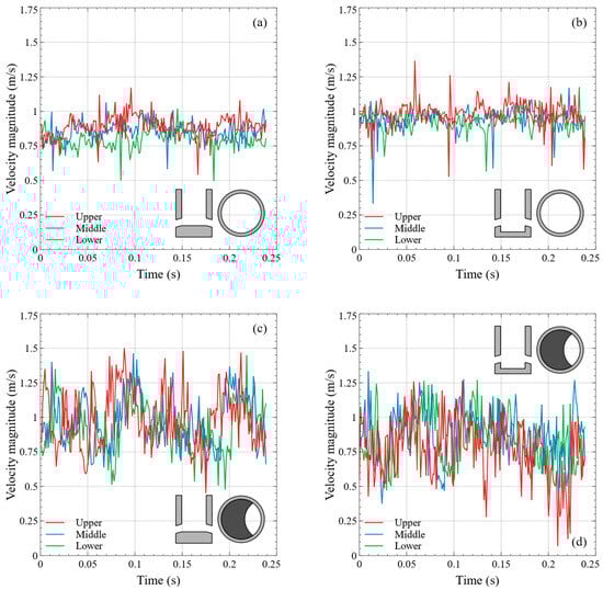
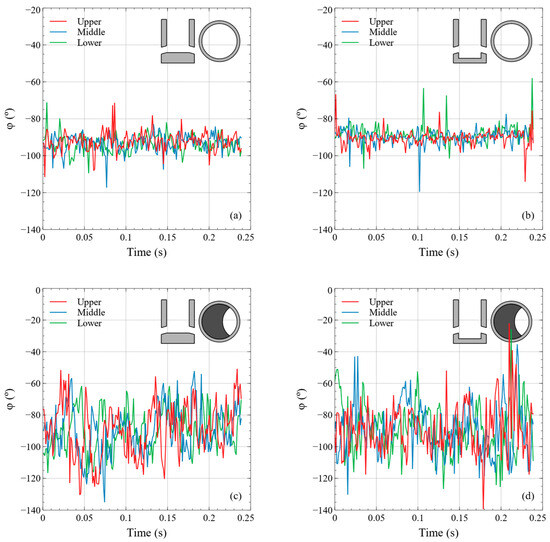

Table 1.
Arithmetic mean and standard deviation of the fluid velocity magnitude and the velocity vector tilt.
Several conclusions can be drawn from Figure 9. The velocity magnitude analysis shows the following: The mean value decreases as the measurement height decreases for all the SEN configurations except at the upper position on the WBSO configuration. For the no-obstruction condition, the mean is lower for the FB design, but this trend reverses for the severe-obstruction condition.
The velocity magnitude standard deviation analysis is as follows: The trend observed in all the configurations is that the standard deviation decreases as the measurement height decreases. Notice that the FBNO and FBSO configurations have almost the same standard deviation. This similarity is also observed in the WBNO and WBSO configurations. On the contrary, the standard deviation for the WBNO configuration is around three times that of the FBNO configuration. A similar proportionality is observed between the WBSO and FBSO conditions.
In addition to the velocity magnitude, the deviation of the velocity vector from the downstream vertical axis was also calculated at the same locations. The mean value of the velocity vector’s vertical tilt shows neither a specific trend nor proportionality between configurations. In addition, the difference among all the values is negligible. However, the standard deviation of the velocity vector’s vertical tilt under the severe-obstruction condition is around three times the value for the same design under the no obstruction condition. The latter can be attributed to the large amount of fluid mixing occurring in the bore.
Along with the statistical analysis, a frequency analysis was also carried out. The power spectral density (PSD) was calculated using the corresponding function in the MATLAB R2023a package on the data shown in Figure 9 and Figure 10. Again, for the sake of space, only the time series belonging to the velocity vector’s vertical tilt at the lower height were analyzed. Figure 11 shows the estimated PSD vs. the frequency for the four SEN configurations. In the plots, near-zero frequency modes were excluded and the expected Nyquist frequency is 200 Hz. Note that the scales are different for the upper and lower panels. The shape of the PSD for the FBNO configuration (Figure 11a) suggests the presence of some periodic fluctuations. In contrast, the plot for the WBNO configuration (Figure 11b) resembles the behavior obtained from a white noise signal. On the other hand, the plots for the FBSO and WBSO configurations (Figure 11c,d) clearly show that the severe-obstruction condition reinforces some periodic behaviors present in the no-obstruction condition or creates new ones with high energy modes.
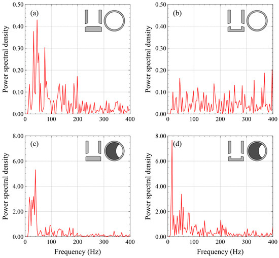
Figure 11.
Frequency analysis of the velocity vector’s tilt time series for the SEN configurations: (a) FBNO, (b) WBNO, (c) FBSO, and (d) WBSO. The SEN design and the SVG clearance are indicated on each panel with sketches.
In summary, the frequency analysis quantitatively corroborates the behavior observed in the high-speed recordings: the SGV increases the turbulence of the flow inside the SEN bore, but the flow displays ordered and periodic fluctuations rather than erratic behavior.
4. Transient Behavior of the SEN Outlet Jets
4.1. Adjustments Made to the SEN
Previous works have studied the control device’s effect on the behavior of the SEN outlet jets by measuring the liquid velocity near the SEN outlets on scaled models using cold water as the working fluid [15,24,28,47]. In those works, the SEN was submerged in the water contained in the mold. The jet velocity was measured using PIV, ultrasonic Doppler velocimetry, and an impeller-velocity probe, among other techniques. The present work adopts a different approach. The SEN outlet jets’ behavior is studied by analyzing transient measurements of the volumetric flow emerging from them. The main purpose of this analysis is not to determine the amount of flow emerging from the outlets but rather to characterize how the flow is distributed at the exit ports. Therefore, a set of customized devices was developed, which, besides dividing the flow emerging from the SEN, allows for coupling with digital flowmeters. Four pieces form this set, and they are shown in Figure 12. Notice that these devices divide the flow into four quarters. The two elements at each side of the SEN are glued together, and subsequently, the new body is glued to the corresponding SEN outlet port.
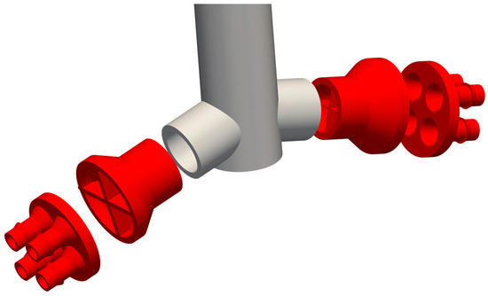
Figure 12.
Customized devices employed for dividing the SEN emerging flow into four quadrants.
Figure 13 shows the experimental rig used for the tests reported in this section. The left panel shows the customized SEN with the devices described previously. As in Section 3, the lower end of the central tube is closed using stoppers with different heights, allowing for both the FB and the WB SEN designs to be generated. However, for convenience, the outlet ports and all the devices were manufactured using a 3D printer with a PLA filament, and their thicknesses were also 3 mm. This panel also shows how rubber pipes connect one coupler to four digital water flow sensors, GR-301 model, from GREDIA (China), shown in the panel on the left of Figure 13. Water exiting from the flow sensors freely falls into the container. The signals generated by the digital flowmeters were acquired using an Arduino Mega microcontroller board, also visible in the left panel of Figure 13.
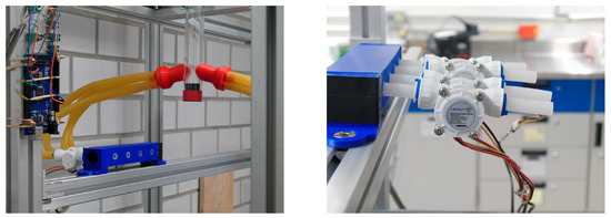
Figure 13.
Experimental rig employed for measuring the volumetric flow at each quadrant and four digital rotational flow meters mounted on a horizontal hub.
The flow sensors employed in this work are turbine-like flowmeters. Therefore, the turbine’s rotation speed is proportional to the volumetric flow rate. Additionally, given that the employed sensors belong to the Class I turbine flow meters (AWWA Standard C701 [48]), the sensors register of the actual rate.
Each flowmeter was calibrated to obtain its characteristic proportionality constant. It was observed that the interval for counting the turbine’s pulses must be at least two seconds to obtain reliable measurements. Thus, the acquisition rate for the volumetric flow signals was one measurement every two seconds. Furthermore, a moving average was applied to the volumetric flow time series to smooth out short-term fluctuations and highlight the longer-term trends.
4.2. Analysis of the Flowmeters Signals
This subsection presents and analyzes the volumetric flow time series obtained from the digital flowmeters using the six SEN configurations described in Figure 4. For clarity, these time series belong to only one of the outlet ports. Since each time series, , represents the volumetric flow leaving the SEN through one of the outlet port’s quadrants, it is crucial to specify the spatial relationship between the SGV plate clearance and the analyzed quadrant. Therefore, the SEN outlet ports quadrants are named after their cardinal direction: Northeast (NE), Northwest (NW), Southeast (SE), and Southwest (SW). The SGV plate’s clearance was located directly above the NE and SE quadrants in all the configurations reported in this section.
Figure 14 and Figure 15 show the transient measurements for the FB and WB SEN designs, respectively. Each panel on these figures uses drawings to indicate the SEN design and the outlet quadrant being studied. In addition, the line color distinguishes the specific SEN configuration. Notice that the scale of the vertical axis of the two graphs in the upper panels of both figures is the same. The same is true for the graphs in the bottom panels. By homogenizing the graph axes’ scales, the time series in Figure 14 and Figure 15 clearly outline the effect of the SGV clearance on how the volumetric flow distributes among each quadrant of the exit port. It is also visible that the effect of the SGV clearance on the SEN outlet jets changes substantially depending on the SEN bottom design.
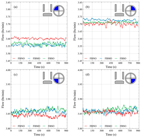
Figure 14.
Time series of the volumetric flow at each quadrant for the FB design and the six SEN configurations. The SEN design and the port quadrant are indicated on each panel with sketches. (a) NW quadrant (b) NE quadrant (c) SW quadrant (d) SE quadrant.
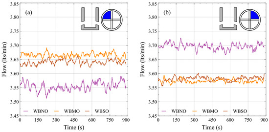
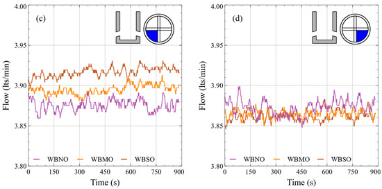
Figure 15.
Time series of the volumetric flow at each quadrant for the WB design and the six SEN configurations. The SEN design and the port quadrant are indicated on each panel with sketches. (a) NW quadrant (b) NE quadrant (c) SW quadrant (d) SE quadrant.
To make the qualitatively observable behavior in Figure 14 and Figure 15 quantifiable, let us construct a set of ad hoc statistics. Table 2 reports the arithmetic mean, , the maximum, , and the minimum, , of the flow rate for each time series, . Equations (1)–(4) define the set of four ad hoc statistics, , , , and , employed to describe the behavior observed in Figure 14 and Figure 15, and Table 3 reports the values of these statistics.
Table 2.
Rank statistics of the volumetric flows time series.
Table 3.
Customized statistics defined in Equations (1) through (4).
The statistic expresses the difference between the flows leaving the SEN through the quadrants on the port’s upper half. Similarly, , , and represent the difference in the flows leaving the SEN through the quadrants on the lower half, the half on the left side, and the half on the right side, respectively.
Previous works devoted to the study of the influence of the bottom configuration on the spread of the jets emerging from SENs found that the WB design produces the broadest jets [45,46]. Those works attributed this feature to the difference between the flow patterns at the SEN’s bottom zone. Based on the results of numerical simulations, they highlighted the difference between the halves on the left and right-hand sides of the jets emerging from the SEN outlet ports. With the data reported in Table 3, the sum of the statistics and for the FBNO configuration is 12.8 and 17.2 for the WBNO configuration. This calculation supports the premise raised in those works.
For the FB design, the data in Table 3 show that modifying the SGV plate’s clearance has little influence on the differences in the outlet port’s south and east halves. However, increasing the turbulence inside the SEN (by reducing the SGV plate clearance) increases the differences in the outlet port’s north and west halves. This behavior can be explained as follows. Increasing turbulence inside the SEN promotes the constant presence of two counter-rotating vortexes in the SEN’s bottom zone (lower panels of Figure 7). By increasing the turbulence, the vortexes’ intensity increases too, but they do not become identical. Recall that the size of the vortex is directly related to the exit flow rate. This assertion is corroborated by the trend observed in Figure 14c,d.
The four statistics, , , , and , show changes in the WB design when the SGV plate clearance is reduced. The changes can be explained by recalling that, when the turbulence inside the bore increases, the intensity of the strongest vortex increases but is pushed downwards and sinks into the pool. The stagnation zone above the ports and below the SGV plate’s clearance also increases its spread. Therefore, the streams flowing through the quadrants on the same half of the SGV plate’s clearance reduce their volumetric flow while the streams on the other half increase their volumetric flow. Additionally, notice that reduces its value by almost half, and the value of increases to just over double. The frequency analysis of the volumetric flow signals was carried out in the same way as in the previous section, and the results are presented in Figure 16 and Figure 17. Again, for clearness, only the analysis of time series belonging to no obstruction and severe obstruction is presented. The results for moderate obstruction are in between the presented extreme cases. Figure 16 and Figure 17 both have the same structure and report the estimated PSD vs. the frequency for the FB and the WB designs, respectively. Notice that all the panels have the same scale for the PSD axis and the frequency range is limited by the Nyquist frequency. The red line displays the results for the no obstruction condition, while the blue line reports the results for the severe obstruction condition.
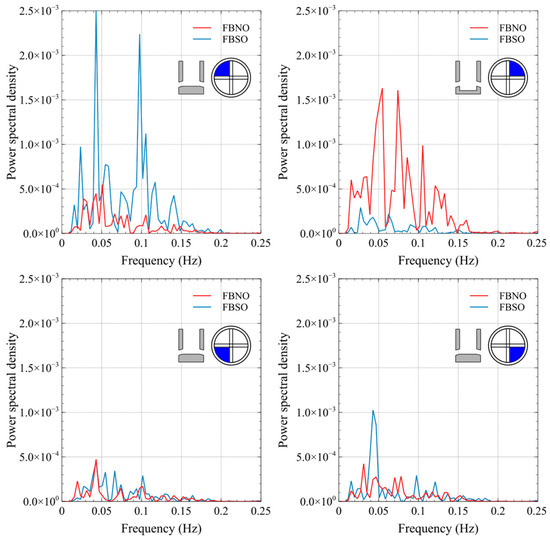
Figure 16.
Frequency analysis of the volumetric flow time series at each quadrant for the FB design and the FBNO and FBSO configurations. The SEN design and the port quadrant are indicated on each panel with sketches.
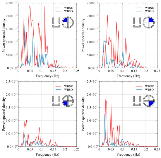
Figure 17.
Frequency analysis of the volumetric flow time series at each quadrant for the WB design and the WBNO and WBSO configurations. The SEN design and the port quadrant are indicated on each panel with sketches.
First, let us analyze the behavior for the no-obstruction condition. The dynamic fluctuations are weaker for the FB design than the WB design. For the FB design, the dynamic behavior in the lower quadrants is quite similar, contrasting with the behavior observed for the upper quadrants. The behavior in the lower quadrants resembles a white noise signal, that is, a quasi-steady-state dynamic behavior with weak random fluctuations. Figure 16 shows periodic fluctuations in both of the upper quadrants, but one has stronger fluctuations. Figure 17 shows periodic fluctuations in all the quadrants for the WB design. Notice that, in this experimental test, the strongest fluctuations are in opposite quadrants, specifically NW and SE.
Now, let us analyze the behavior for the severe-obstruction condition, but recall that the SGV clearance is above the NE and SE quadrants. For the FB design, Figure 16 shows that reducing the SGV clearance led to the following:
- The strength of the fluctuations in the lower quadrants increases, while for the SW it does not change;
- The strength of the fluctuations in the NE quadrant reduces significantly while periodic fluctuations considerably increase in the NW quadrant.
For the WB design, Figure 17 shows that reducing the SGV clearance has the following outcomes:
- The strength of the fluctuations in all the quadrants reduces, but it is much more noticeable in the southern quadrants;
- The strength of periodic fluctuations with specific frequencies increases, which is much more noticeable in the NE and SE quadrants.
The behavior observed in both designs can be understood by recalling that reducing the SGV clearance creates a stagnation zone above the quadrants on the same side of the clearance. This zone, in turn, increases the streams flowing through the quadrants on the opposite half. The overall effect of the SGV can be characterized as a suppression of multiple harmonics enhancing specific frequencies in the exit flow.
4.3. Analysis of the Conic Couplers Effect
The flowmeters mounted on each quadrant of the output ports allow us to measure their bulk flow rate and any slowly changing oscillations. The flowmeters introduce an additional pressure on the port where they are mounted which may lead to a bias in the discharge rate between the two ports. Although a constant pressure imposed on each outlet quadrant would change the total flow rate, this will not affect the measurements of differences in flow rates between quadrants. However, such bias may change the flow pattern inside the SEN’s bore. Visual inspection of the high-speed recordings of the flow structure inside the bore when the flowmeters are mounted shows no qualitative difference with the case of freely discharging flow.
Moreover, the conical pipe couplers that divide the flow into four sections may change the flow pattern expected in the case of SEN without the couplers. The influence of the coupler cannot be readily determined from the experiments. For this reason, we performed numerical simulations using the SPH method. Previous works showed that SPH simulations of weakly compressible fluid satisfactorily reproduce the jet’s structure and the SEN’s internal vortexes [45,46,49]. Details on the numerical parameters and the GPUSPH code are described in [50,51]. Here, we conduct two simulations of FBMO SEN: one without the couplers and one with couplers on both ports. In both cases, water enters through the inlet with a constant velocity . It further accelerates due to gravity and exists freely through the exit ports. The average number of fluid particles was in both simulations. The geometry STL file of the SEN was meshed by unstructured triangular mesh with and discretized with (no couplers) and (with couplers) particles.
To assess the vortex structure inside the SEN, we compare the velocity magnitudes of particles located in a thin slab in the plane centered at . Figure 18 shows the velocity field inside the SEN captured after one second of evolution when the flow is roughly established. It is important to mention that it is expected that fully turbulent flow will settle after 8.0 s, as observed in experimental tests. However, due to excessive computational demand, only one-second numerical simulations were conducted, but we were looking for differences between the pattern with and without couplers. Notice that there is a very similar flow pattern in both cases. This similarity leads us to the conclusion that the fluid freely discharges through the exit ports with the conic couplers does not disrupt the flow pattern inside the SEN.
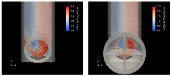
Figure 18.
Velocity of particles along a thin slab centered at for an exit port without (left) and with (right) conic coupler. Note that the SGV clearance is located on the right side of the bore leading to lower speed on the opposite side.
5. Concluding Remarks
This work analyzed how the SGV modifies the dynamic behavior of the fluid flow inside the bore and the SEN exit jets. Through several experimental tests, the frequency analysis of fluid flow fluctuations for six SEN configurations was carried out. For the sake of space, in some cases, only the no-obstruction and severe-obstruction SGV conditions were present. The observed behavior for the moderate-obstruction conditions is in between the presented cases, but the relationship is not linear. For interested readers, we include as Supplementary Material the raw high-speed videos of the flow inside the bore for all the six SEN configurations.
The high-frequency flow fluctuations inside the bore were determined by employing the PIV technique. Also, a low-frequency analysis of the SEN exit jets was carried out using digital flowmeter measurements. These two approaches confirm the observations previously reported for the SEN with no obstruction. Specifically, the WB design produces a dominant, strong vortex, which widens the SEN outlet jets. It was observed that reducing the SGV clearance increases the fluctuations’ amplitude inside the bore, as expected, due to the asymmetry of the entering flow. Despite this, the flow inside the SEN bore displays ordered rather than erratic fluctuations. In addition, it was observed that a stagnation zone below the SGV clearance is formed, which increases the flow on the opposite side of the bore.
The effect of increasing the SGV obstruction is as follows. For the FB design, it promotes the permanent presence of two vortexes at the bottom of the SEN. For the WB design, the dominant vortex is pushed and sunk into the SEN pool, which increases the opening of the SEN outlet jets.
Our findings suggest that current strategies in which the walls of the SEN bore are modified by attaching flow modifiers are unnecessary because the dominant feature is the geometry of the SEN’s bottom section, such as the bottom well. This statement is based on the rounded SEN exit ports used in this work. However, further studies employing ports with other shapes must be carried out.
Finally, several works have reported that the periodic fluctuations inside the mold are found in the 0.5–3.0 Hz frequency range. Our analysis does not cover this range. However, a further study with a new technique for measuring the SEN outlet jet fluctuations in this range is necessary for identifying possible resonant frequencies.
Supplementary Materials
The following supporting information can be downloaded at: https://www.mdpi.com/article/10.3390/fluids9010030/s1, Video S1: Flow pattern inside the bore for the FBNO configuration; Video S2: Flow pattern inside the bore for the FBMO configuration; Video S3: Flow pattern inside the bore for the FBSO configuration; Video S4: Flow pattern inside the bore for the WBNO configuration; Video S5: Flow pattern inside the bore for the WBMO configuration; Video S6: Flow pattern inside the bore for the WBSO configuration.
Author Contributions
Conceptualization, J.G.-T., R.M.-T. and R.G; methodology, J.G.-T., R.M.-T., C.A.R.-R. and R.G.; experimental tests, J.G.-T., R.M.-T. and F.C.-d.-l.-T.; PIV calculations, J.G.-T., F.C.-d.-l.-T. and R.G.; writing—original draft preparation, J.G.-T., R.G. and C.A.R.-R.; supervision, J.G.-T., F.C.-d.-l.-T. and R.G.; funding acquisition, J.G.-T., R.G., F.C.-d.-l.-T., C.A.R.-R. and R.M.-T. All authors have read and agreed to the published version of the manuscript.
Funding
This work was supported by Universidad Autonoma Metropolitana, grant number 22703022.
Data Availability Statement
Data are contained within the article and Supplementary Materials.
Acknowledgments
The reconstruction of the fluid velocity field was carried out using the PIVlab software. The hydrodynamic simulations were made with publicly available GPUSPH v5.0 code www.gpusph.org (accessed on 5 June 2023). The authors acknowledge anonymous reviewers’ comments and subjections, which improve the manuscript structure and results presentation.
Conflicts of Interest
The authors declare no conflicts of interest.
Nomenclature
| CCC | Conventional continuous casting |
| CO2 | Carbon dioxide |
| ESP | Endless strip production |
| FB | Flat-bottom SEN |
| FBMO | Flat-bottom SEN with moderate obstruction |
| FBNO | Flat-bottom SEN with no obstruction |
| FBSO | Flat-bottom SEN with severe obstruction |
| NE | Northeast |
| NW | Northwest |
| PIV | Particle image velocimetry |
| PLA | Polylactic acid |
| PSD | Power spectral density |
| PVC | Polyvinyl chloride |
| SE | Southeast |
| SEN | Submerged entry nozzle |
| SGV | Sliding-gate valve |
| SPH | Smoothed particle hydrodynamics |
| SR | Stopper rod |
| SW | Southwest |
| TSC | Thin slab caster |
| WB | Well-bottom SEN |
| WBMO | Well-bottom SEN with moderate obstruction |
| WBNO | Well-bottom SEN with no obstruction |
| WBSO | Well-bottom SEN with severe obstruction |
References
- Birat, J.-P. Society, Materials, and the Environment: The Case of Steel. Metals 2020, 10, 331. [Google Scholar] [CrossRef]
- Holappa, L. A General Vision for Reduction of Energy Consumption and CO2 Emissions from the Steel Industry. Metals 2020, 10, 1117. [Google Scholar] [CrossRef]
- Holappa, L. Challenges and Prospects of Steelmaking towards the Year 2050. Metals 2021, 11, 1978. [Google Scholar] [CrossRef]
- Raabe, D. The Materials Science behind Sustainable Metals and Alloys. Chem. Rev. 2023, 123, 2436–2608. [Google Scholar] [CrossRef]
- Mousa, E.; Wang, C.; Riesbeck, J.; Larsson, M. Biomass Applications in Iron and Steel Industry: An Overview of Challenges and Opportunities. Renew. Sustain. Energy Rev. 2016, 65, 1247–1266. [Google Scholar] [CrossRef]
- Cemernek, D.; Cemernek, S.; Gursch, H.; Pandeshwar, A.; Leitner, T.; Berger, M.; Klösch, G.; Kern, R. Machine Learning in Continuous Casting of Steel: A State-of-the-Art Survey. J. Intell. Manuf. 2022, 33, 1561–1579. [Google Scholar] [CrossRef]
- Merten, D.C.; Hütt, M.-T.; Uygun, Y. Effect of Slab Width on Choice of Appropriate Casting Speed in Steel Production. J. Iron Steel Res. Int. 2022, 29, 71–79. [Google Scholar] [CrossRef]
- Guthrie, R.I.L.; Isac, M.M. Continuous Casting Practices for Steel: Past, Present and Future. Metals 2022, 12, 862. [Google Scholar] [CrossRef]
- Wang, Y.; Zhang, L. Transient Fluid Flow Phenomena during Continuous Casting: Part I—Cast Start. ISIJ Int. 2010, 50, 1777–1782. [Google Scholar] [CrossRef]
- Zhang, Q.-Y.; Wang, X.-H. Numerical Simulation of Influence of Casting Speed Variation on Surface Fluctuation of Molten Steel in Mold. J. Iron Steel Res. Int. 2010, 17, 15–19. [Google Scholar] [CrossRef]
- Kubo, N.; Kubota, J.; Ishii, T. Simulation of Sliding Nozzle Gate Movements for Steel Continuous Casting. ISIJ Int. 2001, 41, 1221–1228. [Google Scholar] [CrossRef]
- Kalter, R.; Tummers, M.J.; Wefers Bettink, J.B.; Righolt, B.W.; Kenjereš, S.; Kleijn, C.R. Aspect Ratio Effects on Fluid Flow Fluctuations in Rectangular Cavities. Metall. Mater. Trans. B 2014, 45, 2186–2193. [Google Scholar] [CrossRef]
- Du, F.; Li, T.; Zeng, Y.; Zhang, K. Influence of Nozzle Design on Flow Characteristic in the Continuous Casting Machinery. Coatings 2022, 12, 631. [Google Scholar] [CrossRef]
- Sambasivam, R. Clogging Resistant Submerged Entry Nozzle Design through Mathematical Modelling. Ironmak. Steelmak. 2006, 33, 439–453. [Google Scholar] [CrossRef]
- Chaudhary, R.; Lee, G.-G.; Thomas, B.G.; Kim, S.-H. Transient Mold Fluid Flow with Well- and Mountain-Bottom Nozzles in Continuous Casting of Steel. Metall. Mater. Trans. B 2008, 39, 870–884. [Google Scholar] [CrossRef]
- Chatterjee, D. CFD Model Study of a New Four-Port Submerged Entry Nozzle for Decreasing the Turbulence in Slab Casting Mold. ISRN Metall. 2013, 2013, 981597. [Google Scholar] [CrossRef]
- Srinivas, P.S.; Singh, A.; Korath, J.M.; Jana, A.K. A Water-Model Experimental Study of Vortex Characteristics Due to Nozzle Clogging in Slab Caster Mould. Ironmak. Steelmak. 2017, 44, 473–485. [Google Scholar] [CrossRef]
- Cho, S.-M.; Thomas, B.G. Electromagnetic Forces in Continuous Casting of Steel Slabs. Metals 2019, 9, 471. [Google Scholar] [CrossRef]
- Bao, Y.; Li, Z.; Zhang, L.; Wu, J.; Ma, D.; Jia, F. Asymmetric Flow Control in a Slab Mold through a New Type of Electromagnetic Field Arrangement. Processes 2021, 9, 1988. [Google Scholar] [CrossRef]
- Li, Z.; Zhang, L.; Bao, Y.; Ma, D.; Wang, E. Influence of the Vertical Pole Parameters on Molten Steel Flow and Meniscus Behavior in a FAC-EMBr Controlled Mold. Metall. Mater. Trans. B 2022, 53, 938–953. [Google Scholar] [CrossRef]
- Schurmann, D.; Glavinić, I.; Willers, B.; Timmel, K.; Eckert, S. Impact of the Electromagnetic Brake Position on the Flow Structure in a Slab Continuous Casting Mold: An Experimental Parameter Study. Metall. Mater. Trans. B 2020, 51, 61–78. [Google Scholar] [CrossRef]
- Kharicha, A.; Vakhrushev, A.; Karimi-Sibaki, E.; Wu, M.; Ludwig, A. Reverse Flows and Flattening of a Submerged Jet under the Action of a Transverse Magnetic Field. Phys. Rev. Fluids 2021, 6, 123701. [Google Scholar] [CrossRef]
- Vakhrushev, A.; Kharicha, A.; Karimi-Sibaki, E.; Wu, M.; Ludwig, A.; Nitzl, G.; Tang, Y.; Hackl, G.; Watzinger, J.; Eckert, S. Generation of Reverse Meniscus Flow by Applying an Electromagnetic Brake. Metall. Mater. Trans. B 2021, 52, 3193–3207. [Google Scholar] [CrossRef]
- Zhang, X.-W.; Jin, X.-L.; Wang, Y.; Deng, K.; Ren, Z.-M. Comparison of Standard k-ε Model and RSM on Three Dimensional Turbulent Flow in the SEN of Slab Continuous Caster Controlled by Slide Gate. ISIJ Int. 2011, 51, 581–587. [Google Scholar] [CrossRef][Green Version]
- Gursoy, K.A.; Yavuz, M.M. Effect of Flow Rate Controllers and Their Opening Levels on Liquid Steel Flow in Continuous Casting Mold. ISIJ Int. 2016, 56, 554–563. [Google Scholar] [CrossRef]
- Thumfart, M.; Hackl, G.; Fellner, W. Water Model Experiments on the Influence of Phase Distribution in the Submerged Entry Nozzle Considering Varying Operating Conditions. Steel Res. Int. 2022, 93, 2100824. [Google Scholar] [CrossRef]
- Bai, H.; Thomas, B.G. Turbulent Flow of Liquid Steel and Argon Bubbles in Slide-Gate Tundish Nozzles: Part II. Effect of Operation Conditions and Nozzle Design. Metall. Mater. Trans. B 2001, 32, 269–284. [Google Scholar] [CrossRef]
- Bai, H.; Thomas, B.G. Turbulent Flow of Liquid Steel and Argon Bubbles in Slide-Gate Tundish Nozzles: Part I. Model Development and Validation. Metall. Mater. Trans. B 2001, 32, 253–267. [Google Scholar] [CrossRef]
- Szekely, J.; Yadoya, R.T. The Physical and Mathematical Modeling of the Flow Field in the Mold Region in Continuous Casting Systems: Part I. Model Studies with Aqueous Systems. Metall. Trans. 1972, 3, 2673–2680. [Google Scholar] [CrossRef]
- Li, G.; Tu, L.; Wang, Q.; Zhang, X.; He, S. Fluid Flow in Continuous Casting Mold for Ultra-Wide Slab. Materials 2023, 16, 1135. [Google Scholar] [CrossRef]
- Mahapatra, R.B.; Brimacombe, J.K.; Samarasekera, I.V.; Walker, N.; Paterson, E.A.; Young, J.D. Mold Behavior and Its Influence on Quality in the Continuous Casting of Steel Slabs: Part I. Industrial Trials, Mold Temperature Measurements, and Mathematical Modeling. Metall. Trans. B 1991, 22, 861–874. [Google Scholar] [CrossRef]
- Shen, J.L.; Chen, D.F.; Xie, X.; Zhang, L.L.; Dong, Z.H.; Long, M.J.; Ruan, X.B. Influences of SEN Structures on Flow Characters, Temperature Field and Shell Distribution in 420 Mm Continuous Casting Mould. Ironmak. Steelmak. 2013, 40, 263–275. [Google Scholar] [CrossRef]
- Cai, C.; Shen, M.; Ji, K.; Zhang, Z.; Liu, Y. Research on the Influence of the Inner Wall Structure of the Continuous Casting Submerged Nozzle on the Stream of Molten Steel. Trans. Indian Inst. Met. 2022, 75, 613–624. [Google Scholar] [CrossRef]
- Zhang, L.; Yang, S.; Cai, K.; Li, J.; Wan, X.; Thomas, B.G. Investigation of Fluid Flow and Steel Cleanliness in the Continuous Casting Strand. Metall. Mater. Trans. B 2007, 38, 63–83. [Google Scholar] [CrossRef]
- Najjar, F.M.; Thomas, B.G.; Hershey, D.E. Numerical Study of Steady Turbulent Flow through Bifurcated Nozzles in Continuous Casting. Metall. Mater. Trans. B 1995, 26, 749–765. [Google Scholar] [CrossRef]
- Gupta, D.; Lahiri, A.K. Water Modelling Study of the Jet Characteristics in a Continuous Casting Mould. Steel Res. Int. 1992, 63, 201–204. [Google Scholar] [CrossRef]
- Zhang, X.-G.; Zhang, W.-X.; Jin, J.-Z.; Evans, J.W. Flow of Steel in Mold Region During Continuous Casting. J. Iron Steel Res. Int. 2007, 14, 30–35. [Google Scholar] [CrossRef]
- Mohammadi-Ghaleni, M.; Asle Zaeem, M.; Smith, J.D.; O’Malley, R. Computational Fluid Dynamics Study of Molten Steel Flow Patterns and Particle–Wall Interactions Inside a Slide-Gate Nozzle by a Hybrid Turbulent Model. Metall. Mater. Trans. B 2016, 47, 3056–3065. [Google Scholar] [CrossRef]
- Lu, H.; Li, B.; Li, J.; Zhong, Y.; Ren, Z.; Lei, Z. Numerical Simulation of In-Mold Electromagnetic Stirring on Slide Gate Caused Bias Flow and Solidification in Slab Continuous Casting. ISIJ Int. 2021, 61, 1860–1871. [Google Scholar] [CrossRef]
- Yang, H.; Olia, H.; Thomas, B.G. Modeling Air Aspiration in Steel Continuous Casting Slide-Gate Nozzles. Metals 2021, 11, 116. [Google Scholar] [CrossRef]
- Chen, K.K.; Rowley, C.W.; Stone, H.A. Vortex Breakdown, Linear Global Instability and Sensitivity of Pipe Bifurcation Flows. J. Fluid Mech. 2017, 815, 257–294. [Google Scholar] [CrossRef]
- Chen, K.K.; Rowley, C.W.; Stone, H.A. Vortex Dynamics in a Pipe T-Junction: Recirculation and Sensitivity. Phys. Fluids 2015, 27, 034107. [Google Scholar] [CrossRef]
- Real, C.; Miranda, R.; Vilchis, C.; Barron, M.; Hoyos, L.; Gonzalez, J. Transient Internal Flow Characterization of a Bifurcated Submerged Entry Nozzle. ISIJ Int. 2006, 46, 1183–1191. [Google Scholar] [CrossRef][Green Version]
- Real-Ramirez, C.A.; Carvajal-Mariscal, I.; Sanchez-Silva, F.; Cervantes-de-la-Torre, F.; Diaz-Montes, J.; Gonzalez-Trejo, J. Three-Dimensional Flow Behavior Inside the Submerged Entry Nozzle. Metall. Mater. Trans. B 2018, 49, 1644–1657. [Google Scholar] [CrossRef]
- Gonzalez-Trejo, J.; Real-Ramirez, C.A.; Miranda-Tello, J.R.; Gabbasov, R.; Carvajal-Mariscal, I.; Sanchez-Silva, F.; Cervantes-de-la-Torre, F. Influence of the Submerged Entry Nozzle’s Bottom Well on the Characteristics of Its Exit Jets. Metals 2021, 11, 398. [Google Scholar] [CrossRef]
- Gonzalez-Trejo, J.; Real-Ramirez, C.A.; Carvajal-Mariscal, I.; Sanchez-Silva, F.; Cervantes-De-La-Torre, F.; Miranda-Tello, R.; Gabbasov, R. Hydrodynamic Analysis of the Flow inside the Submerged Entry Nozzle. Math. Probl. Eng. 2020, 2020, 6267472. [Google Scholar] [CrossRef]
- Javurek, M.; Wincor, R. Bubbly Mold Flow in Continuous Casting: Comparison of Numerical Flow Simulations with Water Model Measurements. Steel Res. Int. 2020, 91, 2000415. [Google Scholar] [CrossRef]
- American Water Works Association. ANSI/AWWA C701-15: Cold-Water Meters—Turbine Type, for Customer Service; American Water Works Association: Denver, CO, USA, 2015. [Google Scholar]
- Real-Ramirez, C.A.; Carvajal-Mariscal, I.; Gonzalez-Trejo, J.; Miranda-Tello, R.; Gabbasov, R.; Sanchez-Silva, F.; Cervantes-de-la-Torre, F. Visualization and Measurement of Turbulent Flow inside a SEN and off the Ports. Rev. Mex. Fis. 2021, 67, 1–10. [Google Scholar] [CrossRef]
- Hérault, A.; Bilotta, G.; Dalrymple, R.A. SPH on GPU with CUDA. J. Hydraul. Res. 2010, 48, 74–79. [Google Scholar] [CrossRef]
- Gabbasov, R.; González-Trejo, J.; Real-Ramírez, C.A.; Molina, M.M.; la Torre, F.C. Evaluation of GPUSPH Code for Simulations of Fluid Injection Through Submerged Entry Nozzle. In Proceedings of the 10th International Conference on Supercomputing in Mexico, Monterrey, Mexico, 25–29 March 2019; Springer International Publishing: Cham, Switzerland, 2019; pp. 218–226. [Google Scholar]


Disclaimer/Publisher’s Note: The statements, opinions and data contained in all publications are solely those of the individual author(s) and contributor(s) and not of MDPI and/or the editor(s). MDPI and/or the editor(s) disclaim responsibility for any injury to people or property resulting from any ideas, methods, instructions or products referred to in the content. |
© 2024 by the authors. Licensee MDPI, Basel, Switzerland. This article is an open access article distributed under the terms and conditions of the Creative Commons Attribution (CC BY) license (https://creativecommons.org/licenses/by/4.0/).