A Parametric 3D Model of Human Airways for Particle Drug Delivery and Deposition

Abstract

The treatment for asthma and chronic obstructive pulmonary disease relies on forced inhalation of drug particles. Their distribution is essential for maximizing the outcomes. Patient-specific computational fluid dynamics (CFD) simulations can be used to optimize these therapies. In this regard, this study focuses on creating a parametric model of the human respiratory tract from which synthetic anatomies for particle deposition analysis through CFD simulation could be derived. A baseline geometry up to the fourth generation of bronchioles was extracted from a CT dataset. Radial basis function (RBF) mesh morphing acting on a dedicated tree structure was used to modify this baseline mesh, extracting 1000 synthetic anatomies. A total of 26 geometrical parameters affecting branch lengths, angles, and diameters were controlled. Morphed models underwent CFD simulations to analyze airflow and particle dynamics. Mesh morphing was crucial in generating high-quality computational grids, with 96% of the synthetic database being immediately suitable for accurate CFD simulations. Variations in wall shear stress, particle accretion rate, and turbulent kinetic energy across different anatomies highlighted the impact of the anatomical shape on drug delivery and deposition. The study successfully demonstrates the potential of tree-structure-based RBF mesh morphing in generating parametric airways for drug delivery studies.

1. Introduction

The exploration of particle deposition in human airways is of paramount importance in advancing the comprehension of aerosol treatment efficacy [1]. The administration of medical drugs via inhalation stands as a prevalent therapeutic approach for managing widespread respiratory conditions such as asthma and chronic obstructive pulmonary disease (COPD) [2,3,4]. However, the complex and variable anatomy of human airways, coupled with the substantial inter-patient morphological variation, significantly contributes to the complexity of particle trajectories during inhalation [5,6]. Despite the potential therapeutic benefits of aerosolized drug delivery, the variability in particle trajectories within the complex architecture of human airways often results in suboptimal drug deposition [5,7]. This non-optimal distribution can lead to unmanaged symptoms and disease progression in patients with respiratory conditions. In this regard, a comprehensive understanding of these phenomena is crucial for tailor-made inhalation therapies to individual patient characteristics, ensuring optimal drug deposition and, consequently, enhanced treatment outcomes [8,9,10].

To unravel the complex fluid dynamics phenomena that govern the transport and deposition of particles in the airways for accurately estimating the regional dose, numerical models have emerged as a powerful solution [11,12,13]. In this regard, computational fluid dynamics (CFD) stands out as a key numerical tool, offering a versatile approach to analyze and simulate complex airflow patterns within the human respiratory system [14,15,16,17]. In the last decade, different authors have exploited numerical tools to model the human airways [18,19,20,21,22,23]. Several studies explored the capabilities of CFD models as a tool to investigate lung injuries [24,25,26] as well as to optimize drug deposition in human airways [22,23,27,28,29,30]. However, the numerical analysis of drug delivery in the respiratory system involves not only the challenges of particle deposition modeling but also considerations of the inherent complexity and time-consuming nature of CFD studies [31,32]. Conducting detailed CFD simulations of patient-specific anatomies is a multifaceted process, encompassing the detailed variations in airway morphology and physiological parameters. In fact, the highly variable and complex anatomy of human airways introduces significant challenges in accurately modeling the airflow and particle trajectories [33,34,35]. Each individual’s airway geometry can highly influence how and where particles deposit, making generalizations difficult. Then, the physical characteristics of the particles themselves, such as size, shape, and density add another layer of complexity [11,36]. These characteristics directly affect the particles’ behavior in the airway flow, influencing factors like inertial impaction, sedimentation, and diffusion. Moreover, the dynamic nature of breathing patterns, encompassing varying flow rates, further complicates predictive modeling. This variability can lead to differing deposition patterns even under similar conditions and must necessarily be accounted for when simulating these phenomena. Moreover, the time-consuming nature of these simulations poses a significant limitation, particularly in urgent clinical cases where timely decision-making is critical. These complexities necessitate sophisticated modeling approaches and make the prediction of particle deposition challenging for respiratory drug delivery studies. In this complex scenario, CFD analyses for particle deposition could benefit from the implementation of mesh morphing techniques to adapt a baseline patient-specific geometry to a wide range of anatomically different models based on the variation of selected morphological parameters, thus significantly reducing computational costs. The importance of using morphing techniques to parameterize the geometry related to anatomical models enabling systematic and controlled shape variation for patient-specific analyses and sensitivity studies is discussed in [37]. In particular, radial basis function (RBF) mesh morphing was already exploited to enhance the CFD modeling and simulation in the cardiovascular field [38,39,40,41,42].

In this context, our study focused on addressing the challenges previously described by deriving a parametric model of the human respiratory tract capable of generating new synthetic patient-specific geometries on which the representation of the airflow and the particle deposition of the drug could be derived. In this work, we aimed to translate the solution efficacy of RBF mesh morphing to control the shape and size of the upper part and the first three generations of the respiratory tract. In particular, we started with a patient-specific anatomy that we used as baseline geometry to represent different human airways. The mesh of the respiratory tract was created, and its surface portion was subdivided into multiple regions. In order to control each portion of the model, the respiratory tract from the mouth to the fourth generation was described by a set of geometrical parameters. These geometrical parameters consisted of bend radius, diameters, areas, bifurcation angles, and branch lengths. A novel approach based on a specific radial basis functions mesh morphing algorithm acting on the surface computational grid, restructured into a tree-like framework, was implemented to artificially vary the anatomy up to the third generation. It acts recurrently, adapting each part of the parametric model at every iteration according to the provided input parameters. The airflow and particle parameters most relevant for calculating flow patterns and drug deposition in the human respiratory system were identified. These include particle diameter, flow rate, and injection velocity. The most occurring ranges of shape and physical parameters were determined. A total of 1000 different configurations of the input parameters were created. The quality of the grid for each new synthetic patient was checked, and CFD simulations for particle deposition were conducted.

2. Materials and Methods

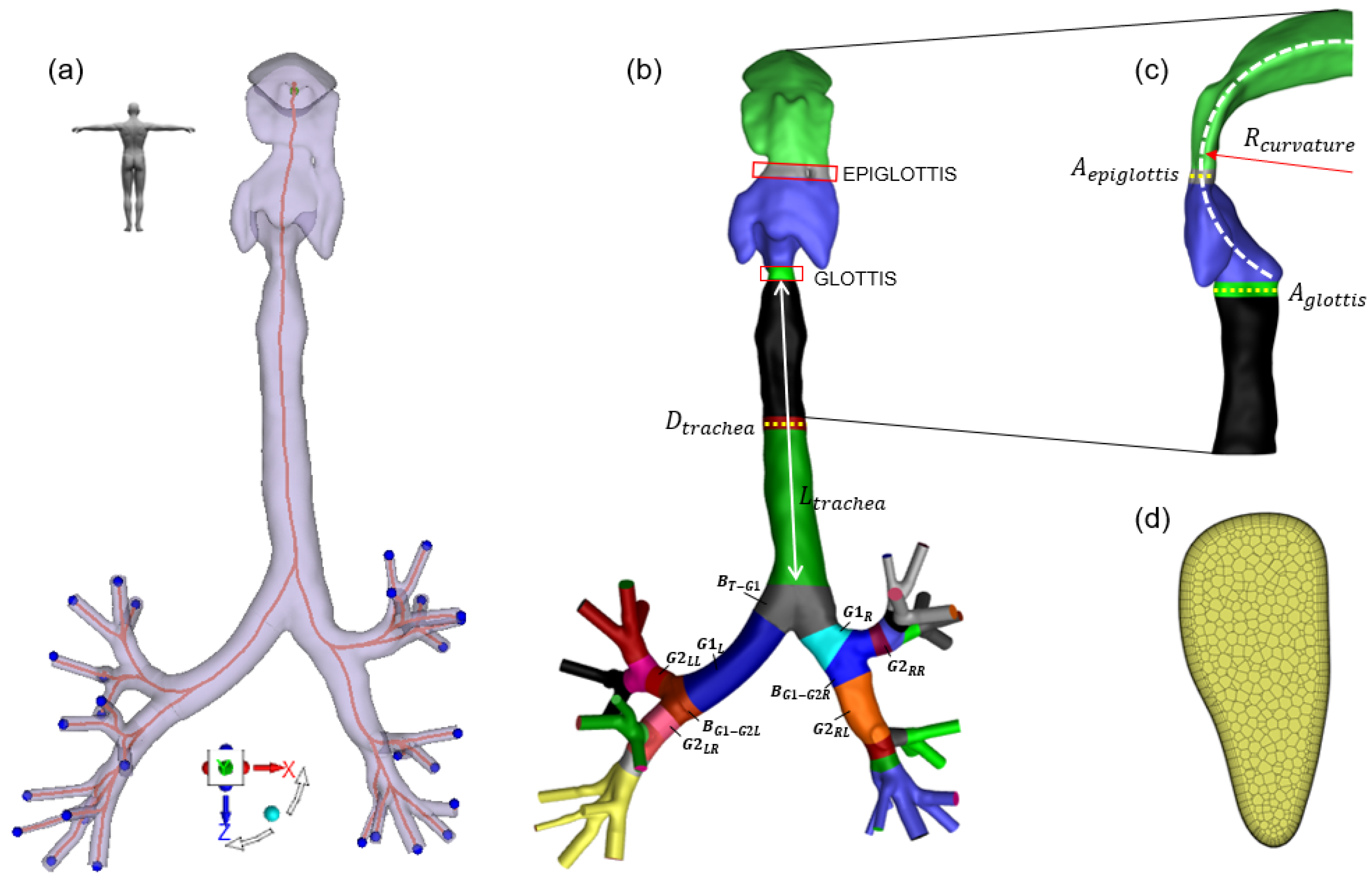
2.1. Baseline Geometry and Centerline Extraction

A CT dataset of a subject volunteer (male, 47 years old) was selected to extract the three-dimensional geometry of the human airways. The dataset was already used in other studies [18,23]. The images were segmented using thresholding methods [43] and then manually refined to obtain the anatomy of interest. The entire human respiratory system comprises 23 generations of airway branches. Asgari et al. [44] conducted a study on the deposition of aerosol microparticles in a realistic lung model spanning from the mouth to the sixth-generation bronchioles. Their findings indicated that aerosol deposition in the case of micron-sized particles predominantly occurs in the superior regions of the airways. For these reasons, in this work, only the upper and central parts of the respiratory tract have been considered, and the segmentation was performed up to the fourth generation of bronchioles, as shown in Figure 1a. To ensure a fully developed flow in the outflow zones, the last segments of the bronchial branches were elongated into pipes of uniform cross-section for a length of 4 times the diameter. Subsequently, the centerline of the model was extracted using VMTK [45] through Voronoi diagrams [46] after automatic detection of the inlet and outlet seed points. The extracted centerline was represented by a set of splines controlled by known points. At the inlets and outlets, the geometry was specifically cut to have a flat surface perpendicular to the centerline, suitable for setting the inflow and outflow boundary conditions of the CFD model. The parameter related to the diameter of each tract was extracted using the same approach proposed in [47]. Briefly, 100 cutting planes perpendicular to the centerline were obtained on each branch. For each branch, 8 segments joining two portions of the perimeter were drawn passing through the center of the plane (i.e., the intersection point of the centerline). These segments spanned angles of 22.5° between them. The average length of the 8 segments constituted the assumed average diameter D${}_i$ of that plane. The average diameter of a given tract was instead defined as:

$$\mathbf{D}=mean\left\{{\mathrm{D}}_1,\dots ,{\mathrm{D}}_{100}\right\}$$

(1)

At each bifurcation of the centerline, a local reference system was inserted to control the bifurcation angle. The origin was placed coincident with the last point before the division of the previous spline into two subsequent splines. The first direction of the reference system was given by the vector connecting the last two points of the spline related to the superior tract. The second direction was determined by computing the normal to the plane passing through the first common point of the bifurcation and the second two control points of each spline. The third direction was obtained through the vector cross-product.

2.2. Mesh Generation and Decomposition

A polyhedral mesh consisting of 1.8 million cells was generated using ANSA pre-processor (BETA CAE Systems, Root, Switzerland). The surface mesh was initially created and an inward extrusion was performed, generating 10 prismatic boundary layers required to accurately predict the wall boundary flow, as shown in Figure 1d. The surface mesh was subsequently partitioned into different sections to uniquely identify the anatomical structures of interest, including the glottis, larynx, epiglottis, trachea, and lower bronchi, shown in Figure 1b. From the trachea onwards, for each branching, a computational buffer zone was identified on the surface grid, which included at least 15 surface polyhedral elements along the direction of the airflow. This zone was defined by isolating parts of the surface grid with cutting planes perpendicular to the centerline. Each buffer zone was created with the aim of absorbing the transformations of the computational grid between one domain and the following. After isolating the surface grid, each domain, including the buffer zones, its nodes, and their coordinates, was placed in an organized tree structure using a Python dictionary. Each branch of the tree thus had a pointer to the father domain and to the respective children.

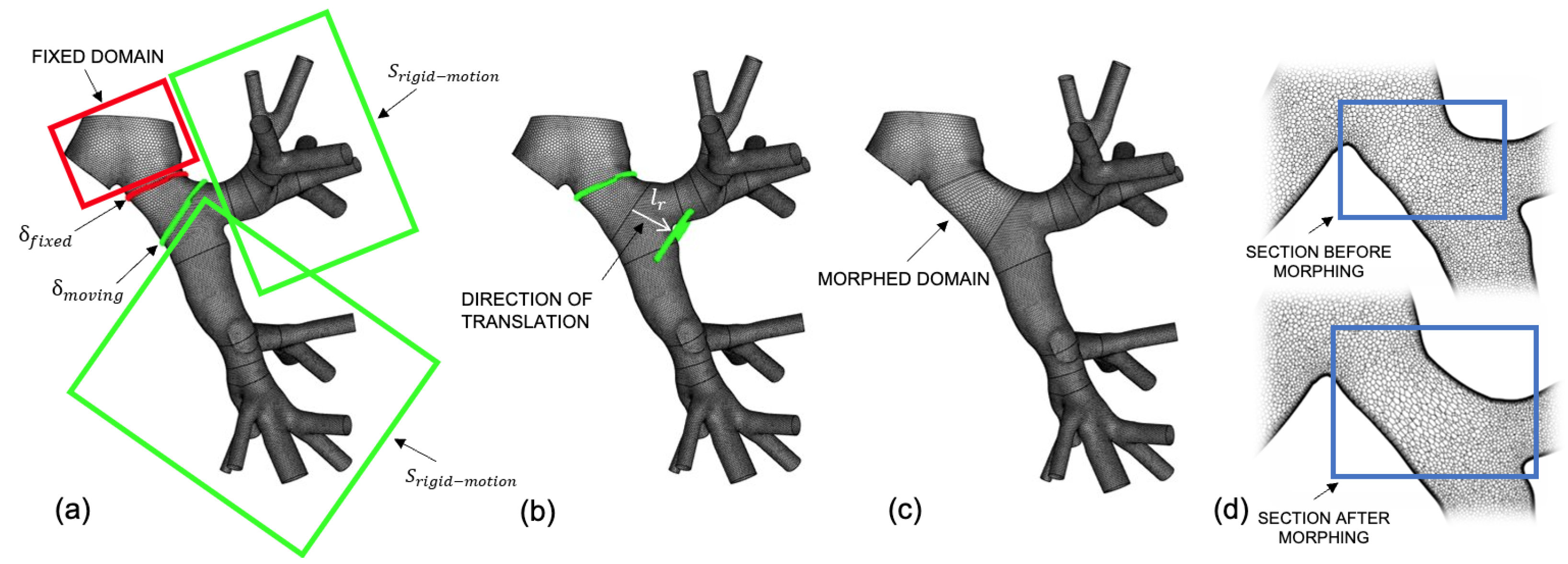
2.3. RBF Mesh Morphing Background

RBF mesh morphing was used to modify the baseline mesh to represent new synthetic anatomies. Among the morphing methods documented in the literature, RBFs are notably recognized for their adaptability to any type of mesh and their superior interpolation capabilities [48]. In particular, RBFs allow the spatial interpolation of a scalar function known at discrete points, called source points (SPs). The displacement of a mesh node in three spatial directions can be described by solving a linear system whose order is equal to the number of SPs used, as detailed in [49]. The interpolation function is the following:

$$s\left(\mathbf{x}\right)=\sum _{i=1}^N{\gamma }_i\phi \left(∥\mathbf{x}-{\mathbf{x}}_{{\mathbf{s}}_{\mathbf{i}}}∥\right)+h\left(\mathbf{x}\right)$$

(2)

where $\mathbf{x}$ represents a generic position in space, ${\mathbf{x}}_{{\mathbf{s}}_{\mathbf{i}}}$ denotes the SP position, $s(·)$ is the function representing a transformation ${\mathbb{R}}^n$→$\mathbb{R}$, $\phi (·)$ is the radial function of order m, ${\gamma }_i$ is the weight, and $h\left(\mathbf{x}\right)$ is a polynomial term with degree $m-1$. The unknowns, which include the polynomial coefficients and the weights ${\gamma }_i$ of the radial functions, are determined by forcing the function to pass through the source point values and imposing an orthogonality condition for the polynomials. The linear problem can be expressed in a matrix format:

$$\left[\begin{array}{cc}\mathbf{M}& \mathbf{P}\\ {\mathbf{P}}^T& \mathbf{0}\end{array}\right]\left\{\begin{array}{c}\gamma \\ \beta \end{array}\right\}=\left\{\begin{array}{c}\mathbf{g}\\ \mathbf{0}\end{array}\right\}$$

(3)

where $\mathbf{M}$ is the interpolation matrix that comprises all the distances between the centers of the RBF ${\mathbf{M}}_{ij}=\phi \left(∥{\mathbf{x}}_{\mathbf{i}}-{\mathbf{x}}_{\mathbf{j}}∥\right)$, $\mathbf{P}$ is the matrix containing the polynomial terms that has for each row j the form ${\mathbf{P}}_j=\left[\begin{array}{c}1,x_{1j},x_{2j},\dots ,x_{nj}\end{array}\right]$, and $\mathbf{g}$ represents the known values at SPs.

Each contribution to the displacement in one of the three directions comes from the following interpolation:

$$\left\{\begin{array}{c}{s}_x\left(\mathbf{x}\right)=\sum _{i=1}^N{\gamma }_i^x\phi \left(∥\mathbf{x}-{\mathbf{x}}_{{\mathbf{s}}_{\mathbf{i}}}∥\right)+{\beta }_1^x+{\beta }_2^{x}x+{\beta }_3^{x}y+{\beta }_4^{x}z\\ s_y\left(\mathbf{x}\right)=\sum _{i=1}^N{\gamma }_i^y\phi \left(∥\mathbf{x}-{\mathbf{x}}_{{\mathbf{s}}_{\mathbf{i}}}∥\right)+{\beta }_1^y+{\beta }_2^{y}x+{\beta }_3^{y}y+{\beta }_4^{y}z\\ s_z\left(\mathbf{x}\right)=\sum _{i=1}^N{\gamma }_i^z\phi \left(∥\mathbf{x}-{\mathbf{x}}_{{\mathbf{s}}_{\mathbf{i}}}∥\right)+{\beta }_1^z+{\beta }_2^{z}x+{\beta }_3^{z}y+{\beta }_4^{z}z\end{array}\right.$$

(4)

When dealing with a mesh, the updated positions of each node can be obtained as:

$${\mathit{x}}_{{\mathit{node}}_{\mathit{new}}}={\mathit{x}}_{\mathit{node}}+\left[\begin{array}{c}{s}_x\left({\mathit{x}}_{\mathit{node}}\right)\\ s_y\left({\mathit{x}}_{\mathit{node}}\right)\\ s_z\left({\mathit{x}}_{\mathit{node}}\right)\end{array}\right]$$

(5)

where ${\mathit{x}}_{{\mathit{node}}_{\mathit{new}}}$ and ${\mathit{x}}_{\mathit{node}}$ represent the vectors containing the updated and original positions of the specified node, respectively.

2.4. RBF Mesh Morphing Application

When applying mesh morphing to the airways, the sections pertaining to the oral cavity, epiglottis, larynx, and glottis were specifically adapted by modifying the curvature radius of the upper respiratory tract or altering the area of the glottis and epiglottis, changing the parameters depicted in Figure 1c. From the trachea to the third generation of bronchi, all structures were controlled using a recursive morphing approach based on the underlying tree structure. The Level Order Traversal technique was used for navigating the tree, whereby all nodes at the same level were completely traversed before moving on to the next level. The function “$\mathit{Traverse}$”, reported below with a pseudocode in Algorithm 1, was used to traverse the tree and prepare the specific morphing operation according to the flag variable (translation, rotation, offset):

Algorithm 1:  $Traverse(S_{morphing},Tree,Flag)$

1: % Initialize the Queue for traversal 2: $Queue.add(Tree.root)$ 3: while  $Queue.IsNotEmpty\left(\right)$  do 4:     $S_{analized}\leftarrow Queue.GetFirstNode\left(\right)$ 5:     $Queue.RemoveFirstNode\left(\right)$ 6:     if $S_{analyzed}=S_{morphing}$ then 7:         if $Flag=“translation”$ then 8:            $Prepare\_morphing\_domains\_translation(S_{analized},Tree,Direction,Magnitude)$ 9:            $\mathbf{Return}$ 10:         else if $Flag=“rotation”$ then 11:            $Prepare\_morphing\_domains\_rotation(S_{analized},Tree,Axis,Angle)$ 12:            $\mathbf{Return}$ 13:         else 14:            $Prepare\_morphing\_domains\_offset(S_{analized},Tree,Diameter)$ 15:            $\mathbf{Return}$ 16:         end if 17:     end if 18:     if $S_{analyzed}.Has\_Children\left(\right)$ then 19:         for $Child\in S_{analyzed}.GetChildren\left(\right)$ do 20:            $Queue.Add\left(Child\right)$ 21:         end for 22:     end if 23: end while

Overall, starting from $n_s$ controlling parameters, $n_s$ morphing procedures were executed within a specific cycle, each acting on a specific section. This approach enabled variations in the bronchial opening angles, enlargement of diameters in each structure, and elongation of the branches belonging to each generation. For every procedure, the surface mesh was stored and used as the starting mesh for the subsequent morphing operation. This recursive process resulted in a completely modified surface mesh based on the $n_s$ controlling parameters. Upon completion of the procedure, a full morphing process was also performed on the volumetric mesh, using the points of the initial surface mesh as SPs, with a displacement determined by the position of the points of the final updated surface mesh [50].

The morphing quality was assessed by deriving the maximum aspect ratio and minimum orthogonal quality [51]. The aspect ratio ($A{R}_i$) of the i-th cell was determined by calculating the ratio between the length of the longest edge and that of the shortest edge. This ratio serves as an indicator of the cell’s geometric perfection. Ideally, in a regular cell, the aspect ratio should be 1. In contrast, for cells with less regular shapes, the aspect ratio exceeds 1, reflecting the disparity in edge lengths. The use of boundary layers, however, results in rather high expected $AR$ values. For these reasons, in addition to the $AR$, the orthogonal quality ($OQ$) is also computed by considering the faces of the individual cells. Two quantities are calculated for each j-th face:

• The normalized dot product of the area vector of a face ($\overrightarrow{A_j}$), whose direction is given by the orientation of the face in space, and a vector from the centroid of the cell to the centroid of that face $\overrightarrow{f_j}$:

  $$O{Q}_{j,1}=\frac{{\overrightarrow{A}}_j·{\overrightarrow{f}}_j}{\left|\overrightarrow{A_j}\right|\left|\overrightarrow{f_j}\right|}$$

  (6)
• The normalized dot product of the area vector of a face ($\overrightarrow{A_j}$) and a vector from the centroid of the cell to the centroid of the adjacent cell that shares that face ($\overrightarrow{c_j}$):

  $$O{Q}_{j,2}=\frac{{\overrightarrow{A}}_j·{\overrightarrow{c}}_j}{\left|{\overrightarrow{A}}_j\right|\left|{\overrightarrow{c}}_j\right|}$$

  (7)

The $OQ$ value of the j-th face is then evaluated as:

$$O{Q}_j=min\left\{O{Q}_{j,1},O{Q}_{j,2}\right\}$$

(8)

Faces with poor $OQ$ will have values closer to 0, while those with optimal $OQ$ will approach a value close to 1.

Below, the morphing transformations performed iteratively on the tree structure of the airways are described in detail.

2.4.1. Translation

The pseudo-code for lengthening or shortening a specific branch associated with a surface $S_i$ delimited by two boundaries ${\delta }_{before}$ and ${\delta }_{after}$ exploiting the tree structure is reported below in Algorithm 2.

Algorithm 2:  $Prepare\_morphing\_domains\_translation(S_{analized},Tree,Direction,Magnitude)$

1: $Copy\_Tree\leftarrow Tree$ 2: ${\delta }_{fixed}\leftarrow S_{analized}.Get\_{\delta }_{before}\left(\right)$ 3: ${\delta }_{fixed}.SetMotion\left(0\right)$ 4: ${\delta }_{moving}\leftarrow S_{analized}.Get\_{\delta }_{after}\left(\right)$ 5: ${\delta }_{moving}.SetDirection\left(Direction\right)$ 6: ${\delta }_{moving}.SetMotion\left(Magnitude\right)$ 7: $S_{rigid\_motion}\leftarrow S_{analized}.GetSubtree\left(\right)$ 8: $S_{fixed}\leftarrow Copy\_Tree.Remove\left([S_{analized},S_{rigid\_motion}]\right)$

The same operations are also described by Figure 2. The portion of the geometry undergoing morphing was only that identified in $S_{analyzed}$. The SPs imposing the motion were contained in ${\delta }_{before}$ (fixed) and ${\delta }_{after}$ (moved). The entire sub-tree from that domain onwards underwent a rigid motion, for which the calculation of RBFs was not necessary. The preceding portion, however, remained fixed.

2.4.2. Rotation

Regarding the rotations, these were set to either increase or reduce the opening angle of each branch up to the third generation. In this morphing action, the buffer designated to absorb the rotation was identified using the same tree traversal algorithm, followed by the identification of its superior and inferior boundaries (in this case, the buffers split into two; thus, it is necessary to uniquely identify both the left and the right contours downstream). The nodes belonging to the upstream boundary were kept fixed in space, while those on the downstream in the left branch underwent a clockwise or counter-clockwise rotation according to the desired opening or closing. The entire downstream surface mesh then experienced a rigid rotation around the initially identified local rotation axis. The rotation applied for opening the right branch of the second generation is shown in Figure 3. A simplified pseudo-code is described below in Algorithm 3:

Algorithm 3:  $Prepare\_morphing\_domains\_rotation(S_{analized},Tree,Axis,Angle)$

1: $Copy\_Tree\leftarrow Tree$ 2: ${\delta }_{fixed}\leftarrow S_{analized}.Get\_{\delta }_{before}\left(\right)$ 3: ${\delta }_{fixed}.SetMotion\left(0\right)$ 4: ${\delta }_{rotating-left}\leftarrow S_{analized}.Get\_{\delta }_{after}\left(\right).GetLeft\left(\right)$ 5: ${\delta }_{rotating-left}.SetAxis\left(Axis\right)$ 6: ${\delta }_{rotating-left}.SetRotation(Angle/2)$ 7: ${\delta }_{rotating-right}\leftarrow S_{analized}.Get\_{\delta }_{after}\left(\right).GetRight\left(\right)$ 8: ${\delta }_{rotating-right}.SetAxis\left(Axis\right)$ 9: ${\delta }_{rotating-right}.SetRotation(Angle/2)$ 10: $S_{rigid-rotation-left}\leftarrow S_{analized}.GetLeftSubtree\left(\right)$ 11: $S_{rigid-rotation-right}\leftarrow S_{analized}.GetRightSubtree\left(\right)$ 12: $S_{fixed}\leftarrow Copy\_Tree.Remove\left([S_{analized},S_{rigid\_rotation\_left},S_{rigid\_rotation\_right}]\right)$

2.4.3. Offset

Regarding the variation of diameter (or area) of each branch, an offset transformation was implemented. All nodes belonging to the selected surface were translated in a direction perpendicular to the surface according to the nodal normal, in order to achieve the desired diameter/area. To avoid abrupt changes between the upstream and downstream domains, the buffer parts acted as domains for absorbing the transformation. The edges that were not affected were indeed kept fixed by imposing a null motion on the corresponding SPs. The offset transformation is shown in Figure 4 and the pseudo-code is reported in Algorithm 4:

Algorithm 4:  $Prepare\_morphing\_domains\_offset(S_{analized},Tree,Diameter)$

1: $Copy\_Tree\leftarrow Tree$ 2: ${\delta }_{fixed}\leftarrow S_{analized}.GetFather\left(\right).Get\_{\delta }_{before}\left(\right)$ 3: if  $$\begin{gathered} S_{analized}.GetFather\left(\right).Get\_{\delta }_{after}\left(\right).GetSize\left(\right)=2 \& \\ {S}_{analized}.GetFather\left(\right).Get\_{\delta }_{after}\left(\right)\left[0\right]=S_{analized}.Get\_{\delta }_{before}\left(\right)\mathbf{then} \end{gathered}$$ 4:     ${\delta }_{fixed}.append(S_{analized}.GetFather\left(\right).Get\_{\delta }_{after}\left(\right)\left[1\right])$ 5: else 6:     ${\delta }_{fixed}.append(S_{analized}.GetFather\left(\right).Get\_{\delta }_{after}\left(\right)\left[0\right])$ 7: end if 8: ${\delta }_{fixed}.append(S_{analized}.GetChildren\left[0\right].Get\_{\delta }_{after}\left(\right).GetRight\left(\right)$ 9: ${\delta }_{fixed}.append(S_{analized}.GetChildren\left[0\right].Get\_{\delta }_{after}\left(\right).GetLeft\left(\right)$ 10: ${\delta }_{fixed}.SetMotion\left(0\right)$ 11: $S_{offset}\leftarrow S_{analyzed}$ 12: $S_{offset}.SetOffset\left(Diameter\right)$

2.5. Synthetic Database Creation

With the purpose of generating new virtual patients, the model underwent $n_s=41$ morphing operations. These corresponded to 15 transformations related to the lengths of the branches, from the trachea to the third generation, 7 rotations for angles concerning each bifurcation, 2 transformations for the area of the epiglottis and glottis, 16 variations of the diameter for the structures from the trachea to the third generation, and 1 parameter related to the curvature of the superior part. However, in order to simplify the control of the model, the parameters related to the diameter were linked together and managed through a single diameter that scaled all the others accordingly, as described in [52]. This morphological relationship had already been discussed in previous publications [53,54]. Globally, 26 geometrical parameters were identified to create a design of experiments and control the parametric model through RBF mesh morphing. The control of the parametric mesh using RBF mesh morphing extended to the structure of the tertiary bronchi. The range of geometrical parameters used was derived from literature [55]. This range was specifically selected to ensure that the geometric variations fall within a physiological range of values and do not result in configurations that are impossible in nature. It is reported in

Table 1. List of geometrical parameters to parameterize the computational model.

Full Parameter Name	Parameter Abbreviation	Minimum Value	Maximum Value
Area of the epiglottis	$A_{epiglottis}$	80 mm${}^2$	340 mm${}^2$
Area of the glottis	$A_{glottis}$	86 mm${}^2$	330 mm${}^2$
Upper airway curvature radius	$R_{curvature}$	45 mm	55 mm
Trachea diameter	$D_{trachea}$	16.5 mm	21.5 mm
Trachea length	$L_{trachea}$	103 mm	132 mm
1st generation angle	${\Theta }_1$	75${}^{\circ }$	105${}^{\circ }$
1st generation left branch length	$L_{G{1}_L}$	51 mm	58 mm
1st generation right branch length	$L_{G{1}_R}$	23 mm	29 mm
2nd generation left branch angle	${\Theta }_{2_L}$	70${}^{\circ }$	90${}^{\circ }$
2nd generation right branch angle	${\Theta }_{2_R}$	75${}^{\circ }$	95${}^{\circ }$
2nd generation left-left branch length	$L_{G{2}_{LL}}$	20 mm	25 mm
2nd generation left-right branch length	$L_{G{2}_{LR}}$	19 mm	25 mm
2nd generation right-left branch length	$L_{G{2}_{RL}}$	28 mm	39 mm
2nd generation right-right branch length	$L_{G{2}_{RR}}$	15 mm	20 mm
3rd generation left-left branch angle	${\Theta }_{3_{LL}}$	80${}^{\circ }$	105${}^{\circ }$
3rd generation left-right branch angle	${\Theta }_{3_{LR}}$	80${}^{\circ }$	105${}^{\circ }$
3rd generation right-left branch angle	${\Theta }_{3_{RL}}$	75${}^{\circ }$	95${}^{\circ }$
3rd generation right-right branch angle	${\Theta }_{3_{RR}}$	80${}^{\circ }$	105${}^{\circ }$
3rd generation left-left-left branch length	$L_{G{3}_{LLL}}$	7 mm	13 mm
3rd generation left-left-right branch length	$L_{G{3}_{LLR}}$	6 mm	10 mm
3rd generation left-right-left branch length	$L_{G{3}_{LRL}}$	7 mm	11 mm
3rd generation left-right-right branch length	$L_{G{3}_{LRR}}$	7 mm	11 mm
3rd generation right-left-left branch length	$L_{G{3}_{RLL}}$	15 mm	19 mm
3rd generation right-left-right branch length	$L_{G{3}_{RLR}}$	8 mm	13 mm
3rd generation right-right-left branch length	$L_{G{3}_{RRL}}$	7 mm	10 mm
3rd generation right-right-right branch length	$L_{G{3}_{RRR}}$	7 mm	10 mm

. A Latin hypercube method [56] was used to generate 1000 synthetic anatomies ready for CFD simulation.

2.6. CFD Settings

The airflow is driven by a differential pressure between the mouth (acting as inlet) and the terminal branches of the airways (serving as outlet). A Dirichlet boundary condition consisting of a parametric inflow velocity was imposed at the level of the mouth, and no-slip boundary conditions were assumed on the solid walls [57]. Each outlet section was named according to the specific lung segment it supplied air to. We hypothesized a simplified uniformly distributed zero pressure at the outlets, a standard practice often adopted in computational analysis of the human airways [58,59]. We assume no effects caused by the mucus generally present on the airway layers [60]. The Navier–Stokes equations for a steady-state case were solved using the second-order upwind momentum SIMPLE scheme, and the pressure-velocity coupling method was adopted. The following mass conservation equation was solved:

$$\nabla ·\left(\rho \overrightarrow{u}\right)=0$$

(9)

where $\rho$ is the density, and u is the air flow velocity.

On the other side, conservation of momentum was described by:

$$\nabla ·\left(\rho \overrightarrow{u}\overrightarrow{u}\right)=-\nabla p+\nabla ·\left(\overline{\overline{\tau }}\right)+\rho \overrightarrow{g}$$

(10)

where p is the static pressure, $\overline{\tau }$ is the stress tensor, and $\rho \overrightarrow{g}$ is the gravitational body force. No external body force arising from the interaction with the dispersed phase was considered in this one-way coupling. The air was assumed with density $\rho$ = 1.225 kg/m${}^3$ and a viscosity of $\mu$ = 1.8 × 10${}^{-5}$ kg/(m s).

Not having experimental data to optimize the turbulent model to be used, the transition SST model was here employed. It was often defined as the best choice for predicting inhalation velocity profiles and turbulent kinetic energy [61,62]. This model is based on the coupling of the SST k-$\omega$ transport equations with one additional equation for the intermittency and one for the transition onset criteria. The transport equation for the intermittency $\gamma$ is defined as:

$$\frac{\partial \left(\rho U_j\gamma \right)}{\partial x_j}=P_{\gamma 1}-E_{\gamma 1}+P_{\gamma 2}-E_{\gamma 2}+\frac{\partial }{\partial x_j}\left[\left(\mu +\frac{{\mu }_t}{{\sigma }_{\gamma }}\right)\frac{\partial \gamma }{\partial x_j}\right]$$

(11)

where the transition sources are defined as:

$$P_{\gamma 1}=C_{a1}{F}_{\mathrm{length}}\rho S{\left[\gamma F_{\mathrm{onset}}\right]}^{c_{\gamma 3}}$$

(12)

and

$$E_{\gamma 1}=C_{e1}{P}_{\gamma 1}\gamma$$

(13)

where S is the strain rate magnitude, $F_{length}$ is an empirical correlation that controls the length of the transition region, $C_{a1}$ = 2, and $C_{e1}$ = 1. The destruction sources are defined as follows:

$$P_{\gamma 2}=C_{a2}\rho \Omega \gamma F_{\mathrm{turb}}$$

(14)

$$E_{\gamma 2}=C_{e2}{P}_{\gamma 2}\gamma$$

(15)

where $\Omega$ is the vorticity magnitude. The following function controls the transaction offset:

$$R_{e_V}=\frac{\rho y^{2}S}{\mu }$$

(16)

$$R_T=\frac{\rho k}{\mu \omega }$$

(17)

$$F_{\mathrm{onset}1}=\frac{R{e}_v}{2193R{e}_{\theta c}}$$

(18)

$$F_{\mathrm{onset}2}=min\left(max\left(F_{\mathrm{onset}1},F_{\mathrm{onset}1}^4\right),2.0\right)$$

(19)

$$F_{\mathrm{onset}3}=max\left(1-{\left(\frac{R_T}{25}\right)}^3,0\right)$$

(20)

$$F_{\mathrm{onset}}=max\left(F_{\mathrm{onset}2}-F_{\mathrm{onset}3},0\right)$$

(21)

$$F_{\mathrm{turb}}=e^{-{\left(\frac{R_T}{4}\right)}^4}$$

(22)

where y is the wall distance, and $R{e}_{\theta c}$ is the critical Reynolds number, where the intermittency first starts to increase in the boundary layer. The remaining constants for the intermittency equation are $C_{a2}$ = 0.06, $C_{e2}$ = 50, $c_{\gamma 3}$ = 0.5, and ${\sigma }_{\gamma }$ = 1. The transport equation for the transition momentum thickness Reynolds number ${\tilde{R}}_{\theta t}$ is:

$$\frac{\partial \left(\rho U_j{\tilde{R}}_{\theta t}\right)}{\partial x_j}=P_{\theta t}+\frac{\partial }{\partial x_j}\left[{\sigma }_{\theta t}\left(\mu +{\mu }_t\right)\frac{\partial {\tilde{R}}_{\theta t}}{\partial x_j}\right]$$

(23)

with:

$$P_{\theta t}=c_{\theta t}\frac{\rho }{t}\left({Re}_{\theta t}-{\widetilde{Re}}_{\theta t}\right)\left(1.0-F_{\theta t}\right)$$

(24)

$$t=\frac{500\mu }{\rho U^2}$$

(25)

$$F_{\theta t}=min\left(max\left(F_{\mathrm{wake}}{e}^{{\left(-\frac{y}{\delta }\right)}^4},1.0-{\left(\frac{\gamma -1/50}{1.0-1/50}\right)}^2\right),1.0\right)$$

(26)

$${\theta }_{BL}=\frac{R{\tilde{e}}_{\theta t}\mu }{\rho U}$$

(27)

$${\delta }_{BL}=\frac{15}{2}{\theta }_{BL}$$

(28)

$$\delta =\frac{50\Omega y}{U}{\delta }_{BL}$$

(29)

$$R{e}_{\omega }=\frac{\rho \omega y^2}{\mu }$$

(30)

$$F_{\mathrm{wake}}=e^{-{\left(\frac{R{e}_{\omega }}{1E+5}\right)}^2}$$

(31)

with $c_{\theta t}$ = 0.03 and $c_{{\sigma }_{\theta t}}$ = 2. The empirical correlations related to ${Re}_{\theta t}$, $F_{length}$, and ${Re}_{\theta c}$ are provided by Langtry and Menter [63]. The transition model interacts with the SST turbulence model by modification of the k-equation as follows:

$$\frac{\partial }{\partial x_i}\left(\rho k{u}_i\right)=\frac{\partial }{\partial x_j}\left({\Gamma }_k\frac{\partial k}{\partial x_j}\right)+G_k^{*}-Y_k^{*}+S_k$$

(32)

$$G_k^{*}={\gamma }_{eff}{\tilde{G}}_k$$

(33)

$$Y_k^{*}=min\left(max\left({\gamma }_{eff},0.1\right),1.0\right)Y_k$$

(34)

where ${\tilde{G}}_k$ and $Y_k$ are the original production and destruction terms for the SST model. For the air phase, the system of equations were numerically solved by using the finite-volume approach in ANSYS Fluent v. 221.

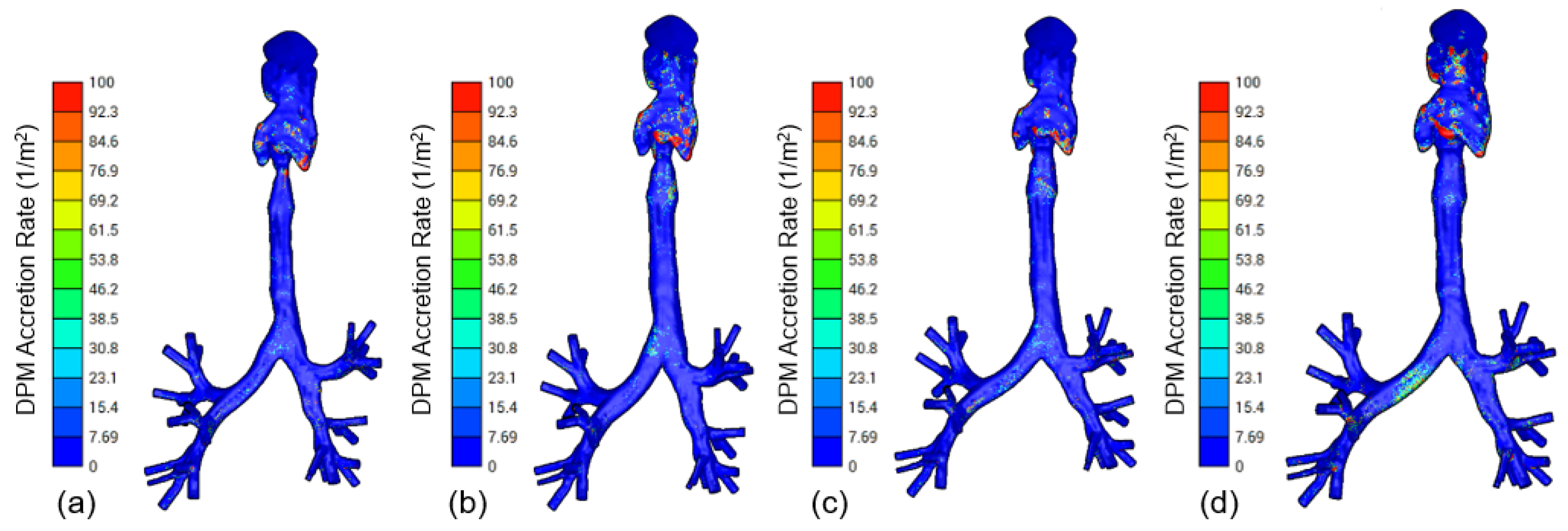
2.7. Discrete Phase Model

The discrete phase model (DPM) was included by defining the initial position, velocity, size, and temperature of drug particles. These initial conditions along with the physical properties of the discrete phase were used for the initialization of the particle trajectory. No heat/mass transfer calculations were considered. The drug particles were assumed as smooth spheres without and with a paramagnetic core (the shell–core particles). The DPM was solved through a one-way coupling principle, accounting for particle movement within the airflow while disregarding the impact of particles on the airflow itself [21]. The trajectory of a discrete phase particle was predicted by integrating the force balance on the particle, written in a Lagrangian reference frame. This force balance is equal to the particle inertia with the forces acting on the particle and can be written as:

$$m_p\frac{d{\overrightarrow{u}}_p}{dt}=m_p\frac{\overrightarrow{u}-{\overrightarrow{u}}_p}{{\tau }_r}+m_p\frac{\overrightarrow{g}\left({\rho }_p-\rho \right)}{{\rho }_p}$$

(35)

where $m_p$ is the particle mass, $\overrightarrow{u}$ is the air phase velocity, ${\overrightarrow{u}}_p$ is the particle velocity, $\rho$ is the fluid density, ${\rho }_p$ is the particle density, and $m_p\frac{\overrightarrow{u}-{\overrightarrow{u}}_p}{{\tau }_r}$ is the drag force with the ${\tau }_r$ particle relaxation time evaluated as:

$${\tau }_r=\frac{{\rho }_p{d}_p^2}{18\mu }\frac{24}{C_{d}Re}$$

(36)

where $\mu$ is the molecular viscosity of the fluid, $d_p$ is the particle diameter, $C_d$ is the drag coefficient, and $Re$ is the relative Reynolds number defined as:

$$Re\equiv \frac{\rho d_p\left|{\overrightarrow{u}}_p-\overrightarrow{u}\right|}{\mu }$$

(37)

The inlet plane at the level of the mouth was selected as input surface, and a uniform diameter distribution for the drug particle was assumed. Particle diameter ($d_p$), particle flow rate ($Q_p$), and inflow velocity ($v_{in}$) were set as input parameters to evaluate the deposition efficiency for different classes of pharmaceutical particles. The ranges for them were:

• (in the 0.1 µm ≤ $d_p$ ≤ 10 µm )
• (in the 15 L/min ≤ $Q_p$ ≤ 190 L/min )
• (in the 1 m/s ≤ $v_{in}$ ≤ 10 m/s )

For all the extracted geometries and for a combination of particle-related parameters, wall shear stress (WSS), turbulent kinetic energy (TKE), and DPM accretion rate were extracted. Mesh morphing and simulations were performed on a Dell Precision 7820 workstation with 2 16-cores, Intel^® Xeon Gold 5218, and 256 GB RAM.

3. Results

3.1. Mesh Morphing

The morphing algorithm allowed for the automatic generation of computational grids for CFD, removing the need to repeat any manual step from scratch. Maximum aspect ratio and minimum orthogonal quality are reported in the histograms of Figure 5. The RBF interpolation methods resulted in smooth spatial transformations that preserved the surface mesh quality and the structure of the underlying boundary layers. The volume meshes extracted through mesh morphing were of relatively good quality. Only 47 of them exhibited an orthogonal quality lower than 0.1. Moreover, within these, the elements with the lowest $OQ$ always constituted less than 2% of the total grid elements. When running the simulations, poorly converged runs due to mesh inconsistency were identified and a remeshing scheme was implemented to prepare a new model for performing the computation. Relatively few cases showed poor convergence or crashed mainly due to combinations of the particular parameters, which generated geometry generally difficult to observe in physiological cases. During a testing phase, creating a DoE of 1000 snapshots, 96% of them proved to be valid, without the need for remeshing, for CFD calculation with particle deposition.

3.2. CFD Modeling

Figure 6 presents a quantitative analysis of the WSS along the inner walls of four different virtual patients (

Table 2. List of parameters for deriving the anatomies for which the wall shear stress is reported in Figure 6a–d.

Parameter Name	Model (a)	Model (b)	Model (c)	Model (d)
$A_{epiglottis}$ (mm${}^2$)	179.16	209.90	121.05	146.02
$A_{glottis}$ (mm${}^2$)	168.91	320.89	124.13	182.01
$R_{curvature}$ (mm)	47.47	52.91	50.22	48.93
$D_{trachea}$ (mm)	16.52	18.33	20.98	20.75
$L_{trachea}$ (mm)	126.75	124.34	121.73	105.01
${\Theta }_1$ (${}^{\circ }$)	99.98	80.05	82.40	98.51
$L_{G{1}_L}$ (mm)	52.13	56.24	51.69	51.64
$L_{G{1}_R}$ (mm)	27.04	27.09	27.69	24.31
${\Theta }_{2_L}$ (${}^{\circ }$)	82.47	82.10	78.74	86.20
${\Theta }_{2_R}$ (${}^{\circ }$)	83.33	86.25	90.05	77.39
$L_{G{2}_{LL}}$ (mm)	21.75	23.13	24.28	21.81
$L_{G{2}_{LR}}$ (mm)	19.60	22.93	21.29	23.79
$L_{G{2}_{RL}}$ (mm)	38.14	32.53	35.38	34.65
$L_{G{2}_{RR}}$ (mm)	17.63	16.29	16.54	16.96
${\Theta }_{3_{LL}}$ (${}^{\circ }$)	89.60	93.88	87.01	96.41
${\Theta }_{3_{LR}}$ (${}^{\circ }$)	94.24	91.68	85.83	99.93
${\Theta }_{3_{RL}}$ (${}^{\circ }$)	87.05	88.75	75.38	80.87
${\Theta }_{3_{RR}}$ (${}^{\circ }$)	95.10	101.70	98.95	93.25
$L_{G{3}_{LLL}}$ (mm)	10.79	8.64	10.63	12.14
$L_{G{3}_{LLR}}$ (mm)	9.08	9.10	7.32	6.31
$L_{G{3}_{LRL}}$ (mm)	8.17	10.75	8.32	7.83
$L_{G{3}_{LRR}}$ (mm)	7.33	8.41	8.78	7.04
$L_{G{3}_{RLL}}$ (mm)	17.55	16.96	18.33	16.77
$L_{G{3}_{RLR}}$ (mm)	11.23	10.96	9.07	11.13
$L_{G{3}_{RRL}}$ (mm)	7.35	7.69	7.45	7.34
$L_{G{3}_{RRR}}$ (mm)	9.93	8.94	7.85	8.46
$d_p$ (µm)	2.89	5.13	5.25	7.33
$Q_p$ (L/min)	189.82	105.01	123.29	176.77
$v_{in}$ (m/s)	4.36	4.54	3.39	3.09

). Given the complicated geometry of the lung, which contributes to flow resistance, there is a significant variation in wall shear stress across different lung airway generations. For all the cases, the turbulent kinetic energy reaches its maximum near the larynx, subsequently starting to decrease beginning with the trachea and continually further down towards the lower generations, as shown in Figure 7 for the models created using the values reported in

Table 3. List of parameters for deriving the anatomies for which the turbulent kinetic energy is reported in Figure 7a–d.

Parameter Name	Model (a)	Model (b)	Model (c)	Model (d)
$A_{epiglottis}$ (mm${}^2$)	179.16	209.90	121.05	214.38
$A_{glottis}$ (mm${}^2$)	168.91	320.89	124.13	274.03
$R_{curvature}$ (mm)	47.47	52.91	50.22	48.70
$D_{trachea}$ (mm)	16.52	18.33	20.98	20.99
$L_{trachea}$ (mm)	126.75	124.34	121.73	114.34
${\Theta }_1$ (${}^{\circ }$)	99.98	80.05	82.40	84.09
$L_{G{1}_L}$ (mm)	52.13	56.24	51.69	54.21
$L_{G{1}_R}$ (mm)	27.04	27.09	27.69	26.72
${\Theta }_{2_L}$ (${}^{\circ }$)	82.47	82.10	78.74	88.76
${\Theta }_{2_R}$ (${}^{\circ }$)	83.33	86.25	90.05	76.47
$L_{G{2}_{LL}}$ (mm)	21.75	23.13	24.28	21.08
$L_{G{2}_{LR}}$ (mm)	19.60	22.93	21.29	21.87
$L_{G{2}_{RL}}$ (mm)	38.14	32.53	35.38	37.11
$L_{G{2}_{RR}}$ (mm)	17.63	16.29	16.54	15.21
${\Theta }_{3_{LL}}$ (${}^{\circ }$)	89.60	93.88	87.01	84.60
${\Theta }_{3_{LR}}$ (${}^{\circ }$)	94.24	91.68	85.83	101.65
${\Theta }_{3_{RL}}$ (${}^{\circ }$)	87.05	88.75	75.38	81.02
${\Theta }_{3_{RR}}$ (${}^{\circ }$)	95.10	101.70	98.95	101.25
$L_{G{3}_{LLL}}$ (mm)	10.79	8.64	10.63	10.28
$L_{G{3}_{LLR}}$ (mm)	9.08	9.10	7.32	9.22
$L_{G{3}_{LRL}}$ (mm)	8.17	10.75	8.32	9.53
$L_{G{3}_{LRR}}$ (mm)	7.33	8.41	8.78	9.36
$L_{G{3}_{RLL}}$ (mm)	17.55	16.96	18.33	17.28
$L_{G{3}_{RLR}}$ (mm)	11.23	10.96	9.07	12.57
$L_{G{3}_{RRL}}$ (mm)	7.35	7.69	7.45	9.04
$L_{G{3}_{RRR}}$ (mm)	9.93	8.94	7.85	7.15
$d_p$ (µm)	2.89	5.13	5.25	1.84
$Q_p$ (L/min)	189.82	105.01	123.29	42.47
$v_{in}$ (m/s)	4.36	4.54	3.39	1.21

.

Figure 8 shows the visualization of the particle distribution of different-sized particles for four different cases (

Table 4. List of parameters for deriving the anatomies for which the DPM accretion rate is reported in Figure 8a–d.

Parameter Name	Model (a)	Model (b)	Model (c)	Model (d)
$A_{epiglottis}$ (mm${}^2$)	90.94	121.05	175.30	207.09
$A_{glottis}$ (mm${}^2$)	145.64	124.13	124.81	338.24
$R_{curvature}$ (mm)	48.25	50.22	47.72	46.29
$D_{trachea}$ (mm)	16.80	20.98	18.78	18.32
$L_{trachea}$ (mm)	111.38	121.73	122.64	105.05
${\Theta }_1$ (${}^{\circ }$)	80.00	82.40	99.93	96.62
$L_{G{1}_L}$ (mm)	51.79	51.69	53.75	56.42
$L_{G{1}_R}$ (mm)	26.56	27.69	24.52	26.34
${\Theta }_{2_L}$ (${}^{\circ }$)	76.82	78.74	86.09	79.35
${\Theta }_{2_R}$ (${}^{\circ }$)	86.97	90.05	85.23	86.65
$L_{G{2}_{LL}}$ (mm)	22.35	24.28	22.76	21.70
$L_{G{2}_{LR}}$ (mm)	21.95	21.29	23.47	21.44
$L_{G{2}_{RL}}$ (mm)	33.28	35.38	31.32	36.20
$L_{G{2}_{RR}}$ (mm)	19.56	16.54	15.33	16.77
${\Theta }_{3_{LL}}$ (${}^{\circ }$)	102.64	87.01	83.48	93.17
${\Theta }_{3_{LR}}$ (${}^{\circ }$)	87.55	85.83	100.53	96.38
${\Theta }_{3_{RL}}$ (${}^{\circ }$)	86.36	75.38	85.49	77.47
${\Theta }_{3_{RR}}$ (${}^{\circ }$)	104.86	98.95	83.76	84.02
$L_{G{3}_{LLL}}$ (mm)	11.14	10.63	10.00	12.92
$L_{G{3}_{LLR}}$ (mm)	7.67	7.32	8.33	7.96
$L_{G{3}_{LRL}}$ (mm)	7.16	8.32	7.49	8.10
$L_{G{3}_{LRR}}$ (mm)	10.40	8.78	10.83	9.61
$L_{G{3}_{RLL}}$ (mm)	18.70	18.33	18.89	18.12
$L_{G{3}_{RLR}}$ (mm)	10.57	9.07	10.65	12.01
$L_{G{3}_{RRL}}$ (mm)	9.98	7.45	8.92	9.77
$L_{G{3}_{RRR}}$ (mm)	9.17	7.85	8.83	8.67
$d_p$ (µm)	8.03	5.25	8.46	6.94
$Q_p$ (L/min)	58.43	123.29	152.89	108.11
$v_{in}$ (m/s)	1.23	3.39	1.18	4.65

). Generally, particle deposition varies primarily based on the diameter of the particles. Particles with a smaller diameter tend to deposit more in the downstream generations compared to those with a larger diameter. The accretion rate in the upper domains also appears to increase as the inlet velocity decreases. Particle deposition is dominant in the upper airways, especially depending on the lower flow rates. This demonstrates that variations in anatomical models produce significant and strong effects worthy of consideration.

4. Discussion

Anatomical parameterization can be used either separately or in conjunction with the physical parameters, enabling the swift creation of synthetic models with controlled geometrical variations. This approach is beneficial as it capitalizes on the detailed information derived from a real patient-specific model and employs the strengths of parameterization techniques commonly found in generic models. The ability to morph the geometry is also crucial in cases where there is a need to replicate anomalous situations of small constriction in parts of the respiratory tract due to occlusion phenomena. From an implementation perspective, significant initial effort was needed to accurately partition the mesh and prepare the morphing strategy. However, once the scripts were finalized, the process became fully automated, enabling the creation of an unlimited number of synthetic models by simply selecting the desired combination of input geometrical parameters. During mesh morphing, the first boundary layers near the wall are not fixed but undergo minimal deformation, typically in the micron range. The ability to preserve the y+ by adopting a harmonic RBF spline is explained in [64]. This adaptability is crucial to accurately reproduce new unknown geometries while maintaining good mesh quality for accurate CFD simulations, particularly for capturing near-wall phenomena. Concerning the morphing results, it should be noted that although the $OQ$ (orthogonal quality) indicates that the degradation of elements is localized in a relatively small number of cells for only a few generated virtual patients, a single distorted element can be sufficient to prevent a computational simulation from reaching convergence. The 4% failure rate in mesh morphing can be attributed to a combination of factors. The complexity of the anatomical geometry and the limitations of the radial basis function (RBF) mesh morphing algorithm are significant contributors, especially in areas with high bifurcation where mesh inconsistency after morphing occurred in 7 configurations. Additionally, the global interaction of 26 controlled geometrical parameters sometimes resulted in unrealistic or unphysiologically accurate airway structures, leading to failures in 33 synthetic anatomies. It is important to note that there were no failures associated with inconsistencies in the CFD boundary conditions. These challenges highlight the complexities of mesh morphing and the importance of the remeshing approach in response to these failures. Of course, reducing the morphing failures is essential for better representing complex geometries immediately suitable for CFD simulation. Setting more stringent bounds for the range of geometrical parameters can prevent the creation of unfeasible airway structures. Adopting incremental morphing steps allows for gradual adjustments, ensuring mesh integrity is maintained. Furthermore, it would be appropriate to define relational constraints for the set of parameters, limiting the variations of some based on the value of others on which they might depend [65]. Finally, mesh optimization techniques could further stabilize the grid structure after morphing. The turbulent kinetic energy plot reveals that turbulence occurs immediately beyond the oropharynx region, and it decays quite rapidly after that in all 960 simulated cases, as already shown in [66]. This work highlighted how a tree-structure-based morphing approach could be used to generate patient-specific human airway models for performing fluid dynamics by controlling a set of geometrical parameters. This achievement is particularly important for medical research, especially in drug delivery optimization to understand how a drug might deposit more in some geometries rather than others. Typically, this type of research is performed on a single shape, while patient-specific deviations can have a large impact on the outcome of such research. This type of research is normally executed by hospitals/clinics, pharmaceutical companies, and other companies that provide technical solutions for the healthcare industry. However, particle deposition within the human airways, which bifurcate through as many as 23 generations, is influenced by a considerable number of shape parameters. Modeling this full extent would lead to a prohibitively high number of mesh cells and impractical simulation durations. Consequently, our model contains the initial four generations and allows mesh morphing on the first three. This aspect is rationalized by the observation that inertial impact is dominant in the upper airways and a large percentage of particles is deposited in the upper airways, and beyond the fourth generation, the distribution of flow and particles tends to become more uniform [67].

Limitations and Future Work

While this study marks an important advance in developing patient-specific CFD models for respiratory drug delivery, it is important to acknowledge its constraints. When creating the parametric model, only variations within small-occluded human airways have been considered. However, people with severely constricted airways are in most need of medical treatment. Therefore, future work should extend the ranges of the shape parameters accounting for unhealthy patients as well. Secondly, the model considered here extends up to the fourth generation, and morphing allows controlling up to the third. Several studies have shown that drug deposition also occurs in subsequent generations, especially when considering diameters on the order of a few nanometers [68]. Time-variant inlet profiles could be applied and combined with the parametric model to reproduce the oscillatory respiratory flow [69,70]. A validation of the in silico model’s deposition against in vivo models or phantoms is still missing, although it was beyond the scope of this work [71,72]. In the future, this parametric model will be used to create a database of results to be compressed in order to obtain a reduced-order model related to specific clinical parameters of interest, which are fundamental in the creation of digital twins of the respiratory tract. The current limitations of our study, mainly in the domain of model accuracy and applicability, highlight directions for future research and development. Such refinements are essential steps towards the long-term objective of enhancing drug delivery methods.

5. Conclusions

This work has proposed an approach to control a parametric model of the respiratory tract for obtaining a wide dataset of virtual patients valid for performing fluid dynamics simulations for particle deposition, also including the acting physical variables. The variation of the airway geometry up to the third generation has been controlled. The findings from this research could provide a significant benefit for simulating particle deposition within human patient-specific airways. RBF mesh morphing can be used to automatically create reliable synthetic models for drug delivery analyses. This approach could allow us to gain deeper insights into the complexities of airflow dynamics and particle deposition across different anatomical structures, which is vital for the progression of personalized medical treatments.

References

1. Sorino, C.; Negri, S.; Spanevello, A.; Visca, D.; Scichilone, N. Inhalation therapy devices for the treatment of obstructive lung diseases: The history of inhalers towards the ideal inhaler. Eur. J. Intern. Med. 2020, 75, 15–18. [Google Scholar] [CrossRef]
2. Reddel, H.K.; Bacharier, L.B.; Bateman, E.D.; Brightling, C.E.; Brusselle, G.G.; Buhl, R.; Cruz, A.A.; Duijts, L.; Drazen, J.M.; FitzGerald, J.M.; et al. Global Initiative for Asthma Strategy 2021: Executive Summary and Rationale for Key Changes. Am. J. Respir. Crit. Care Med. 2022, 205, 17–35. [Google Scholar] [CrossRef]
3. Agustí, A.; Celli, B.R.; Criner, G.J.; Halpin, D.; Anzueto, A.; Barnes, P.; Bourbeau, J.; Han, M.K.; Martinez, F.J.; Montes De Oca, M.; et al. Global Initiative for Chronic Obstructive Lung Disease 2023 Report: GOLD Executive Summary. Eur. Respir. J. 2023, 61, 2300239. [Google Scholar] [CrossRef]
4. Baldi, S.; Dellaca, R.; Govoni, L.; Torchio, R.; Aliverti, A.; Pompilio, P.; Corda, L.; Tantucci, C.; Gulotta, C.; Brusasco, V.; et al. Airway distensibility and volume recruitment with lung inflation in COPD. J. Appl. Physiol. 2010, 109, 1019–1026. [Google Scholar] [CrossRef]
5. Donovan, G.M.; Wang, K.C.W.; Shamsuddin, D.; Mann, T.S.; Henry, P.J.; Larcombe, A.N.; Noble, P.B. Pharmacological ablation of the airway smooth muscle layer—Mathematical predictions of functional improvement in asthma. Physiol. Rep. 2020, 8, e14451. [Google Scholar] [CrossRef]
6. Thomas, M.L.; Longest, P.W. Evaluation of the polyhedral mesh style for predicting aerosol deposition in representative models of the conducting airways. J. Aerosol Sci. 2022, 159, 105851. [Google Scholar] [CrossRef]
7. Rahman, M.; Zhao, M.; Islam, M.S.; Dong, K.; Saha, S.C. Nanoparticle transport and deposition in a heterogeneous human lung airway tree: An efficient one path model for CFD simulations. Eur. J. Pharm. Sci. 2022, 177, 106279. [Google Scholar] [PubMed]
8. Longest, P.W.; Tian, G.; Khajeh-Hosseini-Dalasm, N.; Hindle, M. Validating Whole-Airway CFD Predictions of DPI Aerosol Deposition at Multiple Flow Rates. J. Aerosol Med. Pulm. Drug Deliv. 2016, 29, 461–481. [Google Scholar] [CrossRef] [PubMed]
9. Bui, V.K.H.; Moon, J.Y.; Chae, M.; Park, D.; Lee, Y.C. Prediction of aerosol deposition in the human respiratory tract via computational models: A review with recent updates. Atmosphere 2020, 11, 137. [Google Scholar] [CrossRef]
10. Leclerc, L.; Prévôt, N.; Hodin, S.; Delavenne, X.; Mentzel, H.; Schuschnig, U.; Pourchez, J. Acoustic Aerosol Delivery: Assessing of Various Nasal Delivery Techniques and Medical Devices on Intrasinus Drug Deposition. Pharmaceuticals 2023, 16, 135. [Google Scholar] [CrossRef]
11. Hofmann, W. Modelling inhaled particle deposition in the human lung—A review. J. Aerosol Sci. 2011, 42, 693–724. [Google Scholar] [CrossRef]
12. Longest, P.W.; Bass, K.; Dutta, R.; Rani, V.; Thomas, M.L.; El-Achwah, A.; Hindle, M. Use of computational fluid dynamics deposition modeling in respiratory drug delivery. Expert Opin. Drug Deliv. 2019, 16, 7–26. [Google Scholar]
13. Kharat, S.B.; Deoghare, A.B.; Pandey, K.M. Development of human airways model for CFD analysis. Mater. Today Proc. 2018, 5, 12920–12926. [Google Scholar]
14. Leong, S.; Chen, X.; Lee, H.; Wang, D. A review of the implications of computational fluid dynamic studies on nasal airflow and physiology. Rhinology 2010, 48, 139. [Google Scholar] [PubMed]
15. James Ayodele, O.; Ebenezer Oluwatosin, A.; Christian Taiwo, O.; Adebukola Dare, A. Computational Fluid Dynamics Modeling in Respiratory Airways Obstruction: Current Applications and Prospects. Int. J. Biomed. Sci. Eng. 2021, 9, 16. [Google Scholar] [CrossRef]
16. Faizal, W.; Ghazali, N.N.N.; Khor, C.; Badruddin, I.A.; Zainon, M.; Yazid, A.A.; Ibrahim, N.B.; Razi, R.M. Computational fluid dynamics modelling of human upper airway: A review. Comput. Methods Programs Biomed. 2020, 196, 105627. [Google Scholar]
17. Shang, Y.; Dong, J.; Tian, L.; Inthavong, K.; Tu, J. Detailed computational analysis of flow dynamics in an extended respiratory airway model. Clin. Biomech. 2019, 61, 105–111. [Google Scholar]
18. Kenjereš, S.; Tjin, J.L. Numerical simulations of targeted delivery of magnetic drug aerosols in the human upper and central respiratory system: A validation study. R. Soc. Open Sci. 2017, 4, 170873. [Google Scholar] [CrossRef]
19. Tullio, M.; Aliboni, L.; Pennati, F.; Carrinola, R.; Palleschi, A.; Aliverti, A. Computational fluid dynamics of the airways after left-upper pulmonary lobectomy: A case study. Int. J. Numer. Methods Biomed. Eng. 2021, 37, e3462. [Google Scholar] [CrossRef]
20. Tanprasert, S.; Kampeewichean, C.; Shiratori, S.; Piemjaiswang, R.; Chalermsinsuwan, B. Non-spherical drug particle deposition in human airway using computational fluid dynamics and discrete element method. Int. J. Pharm. 2023, 639, 122979. [Google Scholar] [CrossRef]
21. Inthavong, K.; Zhang, K.; Tu, J. Numerical modelling of nanoparticle deposition in the nasal cavity and the tracheobronchial airway. Comput. Methods Biomech. Biomed. Eng. 2011, 14, 633–643. [Google Scholar]
22. Feng, Y.; Zhao, J.; Kleinstreuer, C.; Wang, Q.; Wang, J.; Wu, D.H.; Lin, J. An in silico inter-subject variability study of extra-thoracic morphology effects on inhaled particle transport and deposition. J. Aerosol Sci. 2018, 123, 185–207. [Google Scholar] [CrossRef]
23. Zhang, Z.; Kleinstreuer, C.; Hyun, S. Size-change and deposition of conventional and composite cigarette smoke particles during inhalation in a subject-specific airway model. J. Aerosol Sci. 2012, 46, 34–52. [Google Scholar] [CrossRef]
24. Geitner, C.M.; Köglmeier, L.J.; Frerichs, I.; Langguth, P.; Lindner, M.; Schädler, D.; Weiler, N.; Becher, T.; Wall, W.A. Pressure-and time-dependent alveolar recruitment/derecruitment in a spatially resolved patient-specific computational model for injured human lungs. arXiv 2023, arXiv:2305.14408. [Google Scholar] [CrossRef] [PubMed]
25. Geitner, C.M.; Becher, T.; Frerichs, I.; Weiler, N.; Bates, J.H.T.; Wall, W.A. An approach to study recruitment/derecruitment dynamics in a patient-specific computational model of an injured human lung. Int. J. Numer. Methods Biomed. Eng. 2023, 39, e3745. [Google Scholar] [CrossRef] [PubMed]
26. Radulesco, T.; Meister, L.; Bouchet, G.; Varoquaux, A.; Giordano, J.; Mancini, J.; Dessi, P.; Perrier, P.; Michel, J. Correlations between computational fluid dynamics and clinical evaluation of nasal airway obstruction due to septal deviation: An observational study. Clin. Otolaryngol. 2019, 44, 603–611. [Google Scholar] [CrossRef] [PubMed]
27. Spasov, G.; Rossi, R.; Vanossi, A.; Cottini, C.; Benassi, A. A critical analysis of the CFD-DEM simulation of pharmaceutical aerosols deposition in extra-thoracic airways. Int. J. Pharm. 2022, 629, 122331. [Google Scholar] [CrossRef]
28. Ponzini, R.; Da Vià, R.; Bnà, S.; Cottini, C.; Benassi, A. Coupled CFD-DEM model for dry powder inhalers simulation: Validation and sensitivity analysis for the main model parameters. Powder Technol. 2021, 385, 199–226. [Google Scholar] [CrossRef]
29. Grill, M.J.; Biehler, J.; Wichmann, K.R.; Rudlstorfer, D.; Rixner, M.; Brei, M.; Richter, J.; Bügel, J.; Pischke, N.; Wall, W.A.; et al. In silico high-resolution whole lung model to predict the locally delivered dose of inhaled drugs. arXiv 2023, arXiv:2307.04757. [Google Scholar]
30. Barrio-Perotti, R.; Martín-Fernández, N.; Vigil-Díaz, C.; Walters, K.; Fernández-Tena, A. Predicting particle deposition using a simplified 8-path in silico human lung prototype. J. Breath Res. 2023, 17, 046002. [Google Scholar]
31. Soni, B.; Aliabadi, S. Large-scale CFD simulations of airflow and particle deposition in lung airway. Comput. Fluids 2013, 88, 804–812. [Google Scholar]
32. Benassi, A.; Cottini, C. Numerical simulations for inhalation product development: Achievements and current limitations. ONdrugDelivery 2021, 127, 68–75. [Google Scholar]
33. Shang, Y.; Tian, L.; Fan, Y.; Dong, J.; Inthavong, K.; Tu, J. Effect of morphology on nanoparticle transport and deposition in human upper tracheobronchial airways. J. Comput. Multiph. Flows 2018, 10, 83–96. [Google Scholar]
34. Aghababaie, M.; Suresh, V.; McGlashan, S.; Tawhai, M.; Burrowes, K. In silico prediction of e-cigarette aerosol particle transport and deposition within the airways. In Proceedings of the 2023 45th Annual International Conference of the IEEE Engineering in Medicine & Biology Society (EMBC), Sydney, Australia, 24–27 July 2023; pp. 1–4. [Google Scholar]
35. Farghadan, A.; Coletti, F.; Arzani, A. Topological analysis of particle transport in lung airways: Predicting particle source and destination. Comput. Biol. Med. 2019, 115, 103497. [Google Scholar] [CrossRef]
36. He, Y.; Bayly, A.E.; Hassanpour, A. Coupling CFD-DEM with dynamic meshing: A new approach for fluid-structure interaction in particle-fluid flows. Powder Technol. 2018, 325, 620–631. [Google Scholar]
37. Sigal, I.A.; Yang, H.; Roberts, M.D.; Downs, J.C. Morphing methods to parameterize specimen-specific finite element model geometries. J. Biomech. 2010, 43, 254–262. [Google Scholar] [CrossRef] [PubMed]
38. Capellini, K.; Vignali, E.; Costa, E.; Gasparotti, E.; Biancolini, M.E.; Landini, L.; Positano, V.; Celi, S. Computational fluid dynamic study for aTAA hemodynamics: An integrated image-based and radial basis functions mesh morphing approach. J. Biomech. Eng. 2018, 140, 111007. [Google Scholar] [CrossRef]
39. Capellini, K.; Gasparotti, E.; Cella, U.; Costa, E.; Fanni, B.M.; Groth, C.; Porziani, S.; Biancolini, M.E.; Celi, S. A novel formulation for the study of the ascending aortic fluid dynamics with in vivo data. Med. Eng. Phys. 2021, 91, 68–78. [Google Scholar] [CrossRef]
40. Biancolini, M.E.; Capellini, K.; Costa, E.; Groth, C.; Celi, S. Fast interactive CFD evaluation of hemodynamics assisted by RBF mesh morphing and reduced order models: The case of aTAA modelling. Int. J. Interact. Des. Manuf. (IJIDeM) 2020, 14, 1227–1238. [Google Scholar] [CrossRef]
41. Geronzi, L.; Gasparotti, E.; Capellini, K.; Cella, U.; Groth, C.; Porziani, S.; Chiappa, A.; Celi, S.; Biancolini, M.E. High fidelity fluid-structure interaction by radial basis functions mesh adaption of moving walls: A workflow applied to an aortic valve. J. Comput. Sci. 2021, 51, 101327. [Google Scholar] [CrossRef]
42. Marin-Castrillon, D.M.; Geronzi, L.; Boucher, A.; Lin, S.; Morgant, M.C.; Cochet, A.; Rochette, M.; Leclerc, S.; Ambarki, K.; Jin, N.; et al. Segmentation of the aorta in systolic phase from 4D flow MRI: Multi-atlas vs. deep learning. Magn. Reson. Mater. Phys. Biol. Med. 2023, 36, 687–700. [Google Scholar] [CrossRef] [PubMed]
43. Aykac, D.; Hoffman, E.A.; McLennan, G.; Reinhardt, J.M. Segmentation and analysis of the human airway tree from three-dimensional X-ray CT images. IEEE Trans. Med. Imaging 2003, 22, 940–950. [Google Scholar] [CrossRef] [PubMed]
44. Asgari, M.; Lucci, F.; Kuczaj, A.K. Multispecies aerosol evolution and deposition in a human respiratory tract cast model. J. Aerosol Sci. 2021, 153, 105720. [Google Scholar] [CrossRef]
45. Antiga, L.; Piccinelli, M.; Botti, L.; Ene-Iordache, B.; Remuzzi, A.; Steinman, D.A. An image-based modeling framework for patient-specific computational hemodynamics. Med. Biol. Eng. Comput. 2008, 46, 1097. [Google Scholar]
46. Antiga, L.; Ene-Iordache, B.; Remuzzi, A. Centerline computation and geometric analysis of branching tubular surfaces with application to blood vessel modeling. In Proceedings of the WSCG, Plzen-Bory, Czech Republic, 3–7 February 2003. [Google Scholar]
47. Geronzi, L.; Haigron, P.; Martinez, A.; Yan, K.; Rochette, M.; Bel-Brunon, A.; Porterie, J.; Lin, S.; Marin-Castrillon, D.M.; Lalande, A.; et al. Assessment of shape-based features ability to predict the ascending aortic aneurysm growth. Front. Physiol. 2023, 14, 378. [Google Scholar] [CrossRef]
48. Yu, H.; Xie, T.; Paszczynski, S.; Wilamowski, B.M. Advantages of radial basis function networks for dynamic system design. IEEE Trans. Ind. Electron. 2011, 58, 5438–5450. [Google Scholar] [CrossRef]
49. Biancolini, M.E. Fast Radial Basis Functions for Engineering Applications; Springer: Berlin/Heidelberg, Germany, 2017. [Google Scholar]
50. Geronzi, L.; Martinez, A.; Rochette, M.; Yan, K.; Bel-Brunon, A.; Haigron, P.; Escrig, P.; Tomasi, J.; Daniel, M.; Lalande, A.; et al. Computer-aided shape features extraction and regression models for predicting the ascending aortic aneurysm growth rate. Comput. Biol. Med. 2023, 162, 107052. [Google Scholar] [CrossRef]
51. Sorgente, T.; Biasotti, S.; Manzini, G.; Spagnuolo, M. A Survey of Indicators for Mesh Quality Assessment. In Computer Graphics Forum; Wiley Online Library: Hoboken, NJ, USA, 2023; Volume 42, pp. 461–483. [Google Scholar]
52. Choi, S.; Yoon, S.; Jeon, J.; Zou, C.; Choi, J.; Tawhai, M.H.; Hoffman, E.A.; Delvadia, R.; Babiskin, A.; Walenga, R.; et al. 1D network simulations for evaluating regional flow and pressure distributions in healthy and asthmatic human lungs. J. Appl. Physiol. 2019, 127, 122–133. [Google Scholar] [CrossRef] [PubMed]
53. Choi, S.; Hoffman, E.A.; Wenzel, S.E.; Castro, M.; Fain, S.B.; Jarjour, N.N.; Schiebler, M.L.; Chen, K.; Lin, C.L. Quantitative assessment of multiscale structural and functional alterations in asthmatic populations. J. Appl. Physiol. 2015, 118, 1286–1298. [Google Scholar] [CrossRef]
54. Sauret, V.; Halson, P.M.; Brown, I.W.; Fleming, J.S.; Bailey, A.G. Study of the three-dimensional geometry of the central conducting airways in man using computed tomographic (CT) images. J. Anat. 2002, 200, 123–134. [Google Scholar] [CrossRef]
55. Ahookhosh, K.; Pourmehran, O.; Aminfar, H.; Mohammadpourfard, M.; Sarafraz, M.M.; Hamishehkar, H. Development of human respiratory airway models: A review. Eur. J. Pharm. Sci. 2020, 145, 105233. [Google Scholar] [CrossRef] [PubMed]
56. Stein, M. Large sample properties of simulations using Latin hypercube sampling. Technometrics 1987, 29, 143–151. [Google Scholar] [CrossRef]
57. Islam, M.S.; Saha, S.C.; Sauret, E.; Ong, H.; Young, P.; Gu, Y. Euler–Lagrange approach to investigate respiratory anatomical shape effects on aerosol particle transport and deposition. Toxicol. Res. Appl. 2019, 3, 2397847319894675. [Google Scholar]
58. Luo, H.; Liu, Y. Modeling the bifurcating flow in a CT-scanned human lung airway. J. Biomech. 2008, 41, 2681–2688. [Google Scholar] [CrossRef] [PubMed]
59. Nithiarasu, P.; Hassan, O.; Morgan, K.; Weatherill, N.; Fielder, C.; Whittet, H.; Ebden, P.; Lewis, K. Steady flow through a realistic human upper airway geometry. Int. J. Numer. Methods Fluids 2008, 57, 631–651. [Google Scholar]
60. Tian, G.; Longest, P.W. Development of a CFD boundary condition to model transient vapor absorption in the respiratory airways. J. Biomech. Eng. 2010, 132, 051003. [Google Scholar] [CrossRef]
61. Xu, X.; Wu, J.; Weng, W.; Fu, M. Investigation of inhalation and exhalation flow pattern in a realistic human upper airway model by PIV experiments and CFD simulations. Biomech. Model. Mechanobiol. 2020, 19, 1679–1695. [Google Scholar] [CrossRef] [PubMed]
62. Zhang, Z.; Kleinstreuer, C. Laminar-to-turbulent fluid–nanoparticle dynamics simulations: Model comparisons and nanoparticle-deposition applications. Int. J. Numer. Methods Biomed. Eng. 2011, 27, 1930–1950. [Google Scholar]
63. Langtry, R.B.; Menter, F.R. Correlation-based transition modeling for unstructured parallelized computational fluid dynamics codes. AIAA J. 2009, 47, 2894–2906. [Google Scholar] [CrossRef]
64. Biancolini, M.E.; Chiappa, A.; Cella, U.; Costa, E.; Groth, C.; Porziani, S. Radial basis functions mesh morphing: A comparison between the bi-harmonic spline and the wendland c2 radial function. In Proceedings of the International Conference on Computational Science, Las Vegas, NV, USA, 16–18 December 2020; pp. 294–308. [Google Scholar]
65. Weibel, E. Morphometry of the human lung: The state of the art after two decades. Bull. Eur. Physiopathol. Respir. 1979, 15, 999–1013. [Google Scholar]
66. Kenjereš, S. On recent progress in modelling and simulations of multi-scale transfer of mass, momentum and particles in bio-medical applications. Flow Turbul. Combust. 2016, 96, 837–860. [Google Scholar] [CrossRef]
67. Islam, M.S.; Saha, S.C.; Sauret, E.; Gemci, T.; Gu, Y. Pulmonary aerosol transport and deposition analysis in upper 17 generations of the human respiratory tract. J. Aerosol Sci. 2017, 108, 29–43. [Google Scholar]
68. Rahman, M.M.; Zhao, M.; Islam, M.S.; Dong, K.; Saha, S.C. Aerosol particle transport and deposition in upper and lower airways of infant, child and adult human lungs. Atmosphere 2021, 12, 1402. [Google Scholar] [CrossRef]
69. Gaddam, M.G.; Santhanakrishnan, A. Effects of varying inhalation duration and respiratory rate on human airway flow. Fluids 2021, 6, 221. [Google Scholar] [CrossRef]
70. Piemjaiswang, R.; Shiratori, S.; Chaiwatanarat, T.; Piumsomboon, P.; Chalermsinsuwan, B. Computational fluid dynamics simulation of full breathing cycle for aerosol deposition in trachea: Effect of breathing frequency. J. Taiwan Inst. Chem. Eng. 2019, 97, 66–79. [Google Scholar] [CrossRef]
71. Koullapis, P.; Kassinos, S.C.; Muela, J.; Perez-Segarra, C.; Rigola, J.; Lehmkuhl, O.; Cui, Y.; Sommerfeld, M.; Elcner, J.; Jicha, M.; et al. Regional aerosol deposition in the human airways: The SimInhale benchmark case and a critical assessment of in silico methods. Eur. J. Pharm. Sci. 2018, 113, 77–94. [Google Scholar]
72. Collier, G.J.; Kim, M.; Chung, Y.; Wild, J.M. 3D phase contrast MRI in models of human airways: Validation of computational fluid dynamics simulations of steady inspiratory flow. J. Magn. Reson. Imaging 2018, 48, 1400–1409. [Google Scholar] [CrossRef]
Figure 1. (a) The segmented model with the centerline extracted for all bifurcations up to the fourth generation. (b) Complete model divided into sections represented by different colors controllable through the mesh morphing: the name of the structures up to the second generation is indicated. (c) View of the superior part of the airways with the identified geometrical parameters. (d) Cutting plane from where the computational grid and the boundary layers were visible.
Fluids 09 00027 g001
Figure 2. (a) Identification of edges for translation and of fixed domains with imposed rigid motion. (b) Direction of translation. (c) Mesh after morphing. (d) Effect of the morphing translation on a derived cutting plane along the direction of flow propagation of the airways model.
Fluids 09 00027 g002
Figure 3. (a) Identification of the edges where rotations are applied to morph the buffer domain. The domain before the buffer is fixed, whereas the left branch downstream undergoes a clockwise rotation, and the right branch an anti-clockwise rotation. (b) Rotation of the edges according to the angle theta around the local reference system. (c) Mesh after morphing. (d) Effect of the morphing rotation on a derived cutting plane along the direction of flow propagation of the airways model.
Fluids 09 00027 g003
Figure 4. (a) The offset is applied by translating all nodes related to the surface affected by the diameter variation. (b) Offset direction for the Source Points belonging to the specific modified segment. (c) Mesh after morphing: the offset is absorbed by the upstream and downstream domains, which act as buffer zones. (d) Effect of the morphing offset on a cross-section perpendicular to the centerline of the airways model.
Fluids 09 00027 g004
Figure 5. Evaluation of the morphing quality using (a) maximum aspect ratio and (b) minimum orthogonal quality.
Fluids 09 00027 g005
Figure 6. Assessment of WSS for 4 different configurations of the input variables of the parametric model (ad).
Fluids 09 00027 g006
Figure 7. Assessment of turbulent kinetic energy for 4 different configurations of the input variables of the parametric model (ad).
Fluids 09 00027 g007
Figure 8. Assessment of particle accretion rate for 4 different configurations of the input variables of the parametric model (ad).
Fluids 09 00027 g008