Abstract
The reliable exchange of data is a crucial issue for the loose coupling of computational fluid dynamics (CFD) and computational structural mechanics (CSM) modules in fluid–structure interaction (FSI) applications. This paper presents a comparison between two methods for mapping the traction field across mismatching grids, namely the RIBES method and the preCICE algorithm, both based on radial basis function (RBF) interpolation. The two methods demonstrate different degrees of control over balance preservation during mapping, with the RIBES algorithm exhibiting greater efficacy. Test benches are a parametric double curved geometry and a wind tunnel mock-up. In this second case, forces from mapping are used to load a CSM model to retrieve stress and displacement fields. Differences in FEM results are appreciable although not significant, showing a correlation between the accuracy of balance preservation during data mapping and the structural output.
1. Introduction
The effective and precise combination of computational fluid dynamics (CFD) and computational solid mechanics (CSM) routines is integral to fluid–structure interaction (FSI). Aerodynamic components such as wings, flaps, rudders and stabilizers are characterized by lightweight and flexible structures. Their mechanical behavior and the dynamics of the fluid flow that grazes over them mutually affect each other. Frequently, the flexibility of the structures involved is such that this reciprocal interplay significantly alters the situation from what it would be if the structure were assumed to be rigid. From a scientific and technical perspective, there are numerous examples falling into this category, including wind turbines [1], textile roofs [2], parachutes [3] and both the static and transient [4] dynamics of airplane wings, to name just a few. Examining an aerodynamic component thoroughly requires a comprehensive analysis of the interaction between the two fundamental physics. For instance, if the structural evaluation is conducted statically, the component must be considered in its equilibrium state, accounting for its deformed shape and the corresponding fluid flow. This integration is generally obtained by resorting to one of two main approaches [5]: the tight approach involves the writing of a unique large system of both fluid dynamics and structural mechanics equations whose solution simultaneously updates variables pertaining to the two physics; the loose coupling approach adopts separate solvers for CFD and CSM problems, and boundary conditions are updated iteratively until convergence. Both approaches possess advantages and disadvantages. The tight approach necessitates greater computational resources and expertise, rendering it less prevalent compared to the alternative strategy. Often, it is implemented using in-house codes developed by the user. However, it offers the simultaneous handling of both physics, resulting in faster and more stable convergence [6]. Conversely, the loose coupling method [7] utilizes pre-existing, well-established software to independently solve the two problems. Nevertheless, this approach may encounter convergence difficulties and demands robust and precise data transfer between the associated modules. This data transfer constitutes a significant drawback of the loose method. Typically, CFD and CSM numerical grids do not align, as meshing practices differ between the two domains. Pressures, extracted at the centers of CFD cells, need to be mapped onto CSM nodes and converted to forces. As this process iterates multiple times before convergence, any errors introduced during this data shift are likely to accumulate, potentially leading to solutions deviating significantly from the correct one. Mapping algorithms for surface meshes can be broadly divided into two categories: weighted-residual methods and interpolation methods [8]. Weighted-residual methods involve computing a residual over the problem domain using test functions and setting it equal to zero. The nature of this residual can vary; if it is computed from the pressure fields, the method is known as mortar. This can be standard mortar if the test functions are the common shape functions [9,10] or dual mortar if dual shape functions are used [11]. Area-weighted averaging is suitable for cell-centered data [12,13,14,15], where the test functions exhibit a stepwise behavior from inside to outside a cell. The reaction-force method [16,17] is a mapping method based on a static analysis, using a common discretization between source and target meshes. In this case, the underlying weak formulation is that at the base of FEM itself. Interpolation techniques use polynomials or mathematical series based on the spatial proximity between source and target points. Nearest-neighbor interpolation [18], nearest element interpolation [19], polynomial interpolation [20] and radial basis function interpolation fall into this category. A vast body of literature exists on mapping methods, with notable and comprehensive reviews provided by Smith et al. [21], Franke [22] and others.
The focus of this paper is to compare two data mapping strategies within the context of CFD-CSM data exchange. Both approaches utilize radial basis functions (RBFs) as a crucial component of their algorithms. The first method, introduced in [23], is referred to as the RIBES method, as it was developed to address a key aspect of the RIBES EU research project. RIBES stands for Radial basis functions at fluid Interface Boundaries to Envelope flow results for advanced Structural analysis. Initiated in December 2014 and concluded in December 2016, the project aimed to enhance the methodologies employed in aircraft design. The second method is that included in the preCICE open-source coupling library. PreCICE stands for Precise Code Interaction Coupling Environment [24]; it enables multi-code coupling of existing software for many types of numerical simulations. In the current release of preCICE, the available data mapping methods are limited to those that operate in a black-box manner on point clouds (such as nearest-neighbor mapping and RBF interpolation) or require minimal additional information (like nearest-projection mapping). The present work focuses on the method employing RBF interpolation.
The comparison parameters encompass the criteria for defining a robust and high-quality mapping method. These include load conservation, where force and moment resultants should remain unchanged before and after mapping, with associated vectors aligning in magnitude and direction. Additionally, flexibility is essential, requiring the method to seamlessly handle transfer problems between fine and coarse meshes without requiring ad hoc adjustments. Lastly, performance metrics such as computational time and memory usage must remain within reasonable limits. Comparison benchmarks are the catenoid, introduced in [8] and addressed also in [23], and a straight 1.6 m wide wing, with a root chord of 600 mm and 0.7 as the taper ratio, employed in the wind tunnel experimental campaign within the RIBES project [25,26]. As regards the latter, fluid results from CFD analyses are mapped onto the structural mesh to conduct stress assessments. Finally, another desired requirement for a well-conceived mapping method is the ability to potentially interface with any FEM/CFD solver. In this regard, the tests are conducted using commercial and open-source solvers.
RBF Interpolation
Radial basis functions (RBFs) constitute a central focus in approximation theory [27], which deals with the challenge of approximating complex and usually unknown functions using simpler functions derived from incomplete and scattered data. RBFs stand out as particularly attractive among various interpolating mathematical tools because they enable the generation of an analytical interpolator capable of exactly reproducing specified values at known points in a smooth manner. A unique RBF series can, in fact, manage a substantial quantity of points providing a seamless interpolation devoid of the instability and oscillations commonly associated with high-degree polynomials. This eliminates the necessity for employing specific patterns of point placement or resorting to piecewise interpolation methods, as well as the requirement for organizing points into structured grids. Below, we provide an overview of the mathematical foundation and the terminology related to the RBF problem, without aiming to cover every detail comprehensively. For those interested, we suggest referring to the literature available on both aspects: the purely mathematical [28] and the more practically oriented [29] perspective.
The formulation of an interpolation problem begins with a collection of points in an N-dimensional space, referred to as source points. Each point is linked to a specific field value, whether scalar or vectorial. The sought interpolator provides the field value at any target point within the N-dimensional space, returning the original value if the target location coincides with a source point. The interpolating function above addressed is a collection of radial bases :
where the summation extends to the number of introduced source points. Table 1 lists several of the most common radial bases (or kernels), where and ϵ serves as a shape parameter [30], introduced to accommodate the average grid spacing. In the case of the generalized multiquadratic (GMQ) kernel, the values of and are determined by the user and need to be adjusted according to the specific characteristics of the problem at hand. provides a scalar value because each radial basis is contingent upon the Euclidean distance between points. In case a vectorial field should be reproduced, Equation (1) applies independently to each scalar component of the field. The weights appearing in Equation (1) are determined by imposing the interpolation condition, ensuring that the interpolator precisely reproduces the original values at the source points. In a vector-matrix representation:

Table 1.
Most common radial basis functions.
Here, represents the matrix comprising the radial bases calculated individually for each source point as the target, is the vector containing the given values and represents the vector of unknown weights. To accommodate the representation of a polynomial function , whose degree varies according to the selected kernel [30], it can be incorporated into the series outlined in Equation (1). This inclusion introduces formal complexities into the system described in Equation (2), as additional orthogonality conditions are required to handle the augmented set of unknowns, which now also include the coefficients of the polynomial. Further mathematical consequences pertaining to this extension can be explored in the specialized literature. The method just described is the simplest way of performing an RBF interpolation. However, as is evident, large numbers of nodes lead to large matrices that need to be inverted. Partition of unity techniques [31] can divide a single interpolation problem into several smaller problems that partially overlap, resulting in a consistent reduction in computational running time. It is hardly necessary to observe that RBF interpolation finds wide application in many fields, and it would be extremely belittling not to acknowledge their successful adoption out of a plain interpolation context: from neural networks [32] to computer graphics (surface reconstruction [33]); from mesh morphing [34,35] to image analysis of deformations [36,37]; strain retrieval in non-linear mechanics [38]; and association with reduced order models [39]. RBF mesh morphing has been employed for several applications, from evolutionary optimizations [40] to advanced modelling [41]. RBFs also proved to be a valuable tool to enhance FEM accuracy [42] and, as basis for collocation methods, led to very accurate results for stress retrieval in composite laminates [43].
2. Methods and Results
2.1. The Catenoid
The first test bench used to validate the soundness of the algorithms under comparison was the catenoid [8], a double curvature hull parametrically described by Equation (3):
In this equation, ∈ [0, π] and ∈ [−1.5, 1.5]. The pressure field acting on the catenoid is also given an analytical form:
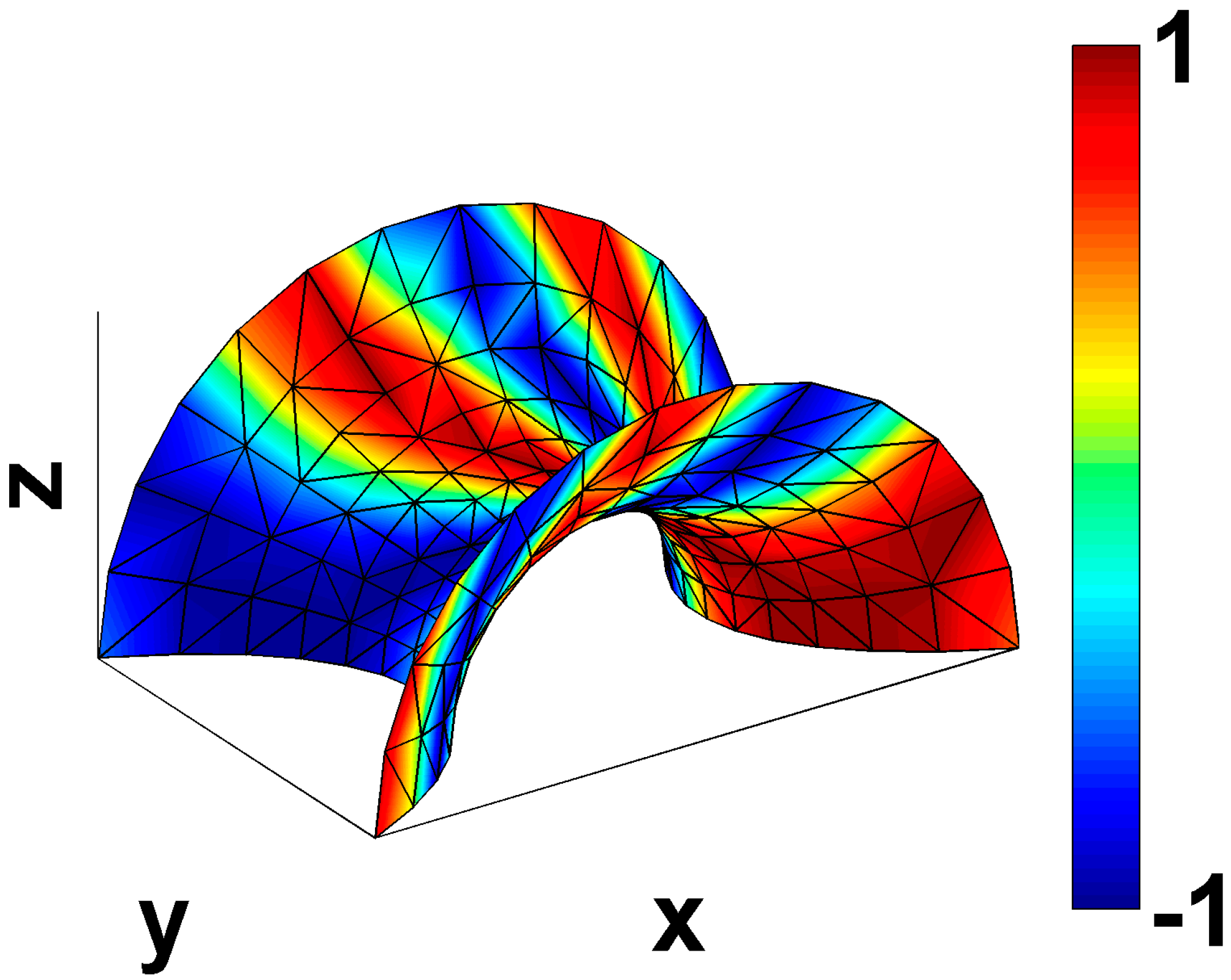
The parametric shell is then discretized into triangular patches, where the total number of nodes or elements indicates the refinement level. Mapping was performed from source to target meshes according to the matchings reported in the rows of Table 2. This process ensures comprehensive coverage of all couplings, encompassing transitions from coarse to fine, from fine to coarse and across similar discretization levels. Figure 1 illustrates the grid, comprising 196 nodes, constructed based on the catenoid geometry. The colormap represents the pressure field in Equation (4).

Table 2.
Row-wise: discretization size of mesh pairs used for mapping.
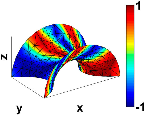
Figure 1.
Grid comprising 196 nodes constructed on the catenoid geometry. Colormap refers to the pressure field.
The RIBES method utilizes RBF interpolation to obtain the source pressure field values at target nodes. In fact, the points on the grid where pressure is known serve as the source sites for an RBF interpolation problem, while the nodes of the second mesh are the target points where pressure needs to be determined. The matrix , introduced in Equation (2), is constructed by inter-correlating points from the source domain, while the vector collects the pointwise values of pressure at those nodes. Upon solving the system, the vector is found, which is then applied to another correlation matrix, linking points across different domains, and resulting in the interpolated pressure values at the target nodes. These values then undergo an optimization process based on fuzzy sets [44] to ensure balance conservation from source to target. Each node of the coarser mesh serves as the center of a spherical fuzzy subset, including a specified number of nodes from the coarser mesh. Correspondingly, identical arrangements of fuzzy subsets are established over the finer mesh, with nodes falling within the same pre-organized spherical volumes. Balance between pairs of homologous subsets across source and target domains is enforced through corrective coefficients that smoothly vary over the target. Determining the appropriate number of points to include in each fuzzy subset is a non-trivial task. While the mathematical properties of fuzzy subsets guarantee translational balance, the sought-after number of nodes may minimize errors in the rotational balance. In most cases involving shell meshes, this minimum lies within the interval , with
where and are the number of points of source and target grids, respectively. For each instance in Table 2, each integer comprising the interval in Equation (5) was employed to tune the correction of RBF interpolation. Only the scenario that exhibited the least rotational imbalance was kept. The code, which executes the described workflow, was scripted using Matlab R2023a. Table 3 summarizes the errors on balance encountered with the RIBES method for the cases in Table 2. The RBF kernel was a linear spline with no polynomial supplement; the pole used for moment calculation was the center of gravity of the target mesh. As expected, greater errors are evident at the extremities of Table 3 where the most dissimilar meshes interconnect. Nevertheless, the maximum error in the magnitude of the moment vector barely exceeds 5%, a level deemed acceptable.

Table 3.
Percentage errors on global resultants, component-wise () and for vectors (). For the catenoid geometry, and employing the RIBES method.
The same tests were repeated using the preCICE algorithm. It should be noted that preCICE offers the user a choice between conservative and consistent mapping approaches. The conservative method takes nodal forces as input and aims to maintain translational balance between the source and target meshes. However, in the case of coarse-to-fine mapping, forces are only applied to a subset of target nodes, chosen based on their proximity to the source nodes. While this configuration may yield satisfactory balance results, it lacks consistency in terms of output, as a continuous pressure field is transformed into a spiky one, with discontinuous variations between zero and peak values. As recommended in the preCICE guide for the mapping of physical (non-cumulative) variables such as pressure, the authors opted for the consistent option, evaluating its performance against balance preservation. In preCICE, consistent mapping can be achieved using either projection-based data mapping or data mapping with RBFs. Since this paper focuses on RBF-based methods, the latter was chosen. This led to a straightforward RBF interpolation problem across different domains with no additional control over global quantity conservation. Table 4 presents the preCICE errors in balance for the catenoid test bench, corresponding to the mesh couplings detailed in Table 2.

Table 4.
Percentage errors on global resultants, component-wise () and for vectors (). For the catenoid geometry, and employing the preCICE algorithm.
The consistent preCICE algorithm introduced discrepancies in balance for both translational and rotational equilibria, which, for the most dissimilar meshes, exceeded 15% of the vector magnitude.
2.2. The RIBES Wing
FSI methodologies and numerical strategies require validation against experimental results. Numerous online databases provide data from both static and dynamic aeroelastic campaigns for code validation (Agard 445.6 [45], HIRENASD [46], EuRAM [47], DLF-F6 [48], Turek FSI benchmark [49]). However, customized measurements are often necessary to address specific aspects of the case being studied, depending on the emphasis during the validation phase. The RIBES project involved fabricating and equipping a wing mock-up for use in a wind tunnel campaign. The RIBES wing has a wingspan of 1600 mm, with CAD and numerical models available online [50]. Comparison between mapping algorithms now encompassed the whole CFD–CSM workflow interrupted after one iteration of a steady-state study. CFD analysis was conducted within the SU2 environment. SU2 is an open-source CFD solver widely used in the aeronautical field due to its high reliability for both compressible and incompressible analyses.
SU2 can solve the compressible Reynolds-Averaged Navier–Stokes (RANS) equations [51], expressed in differential form as
Equation (6) describes the evolution of mass, momentum and energy in a control domain Ω over time t. is the vector of conservative variables, i.e., , where is the fluid density, is the total energy per unit mass, is the flow velocity in a Cartesian coordinate system and is a generic source term. and are the convective and viscous fluxes, respectively.
In this analysis, a “standard air” model was considered. This means that compressibility effects were also included, assuming the air behaved as an ideal gas. An SST turbulence model was enforced, and the same boundary conditions used in the RIBES project were applied: the analysis was steady-state, with Mach number = 0.11762, Angle of attack = 6°, Reynolds number = 1.41 × 10⁶ and Reynolds length = 0.5153.
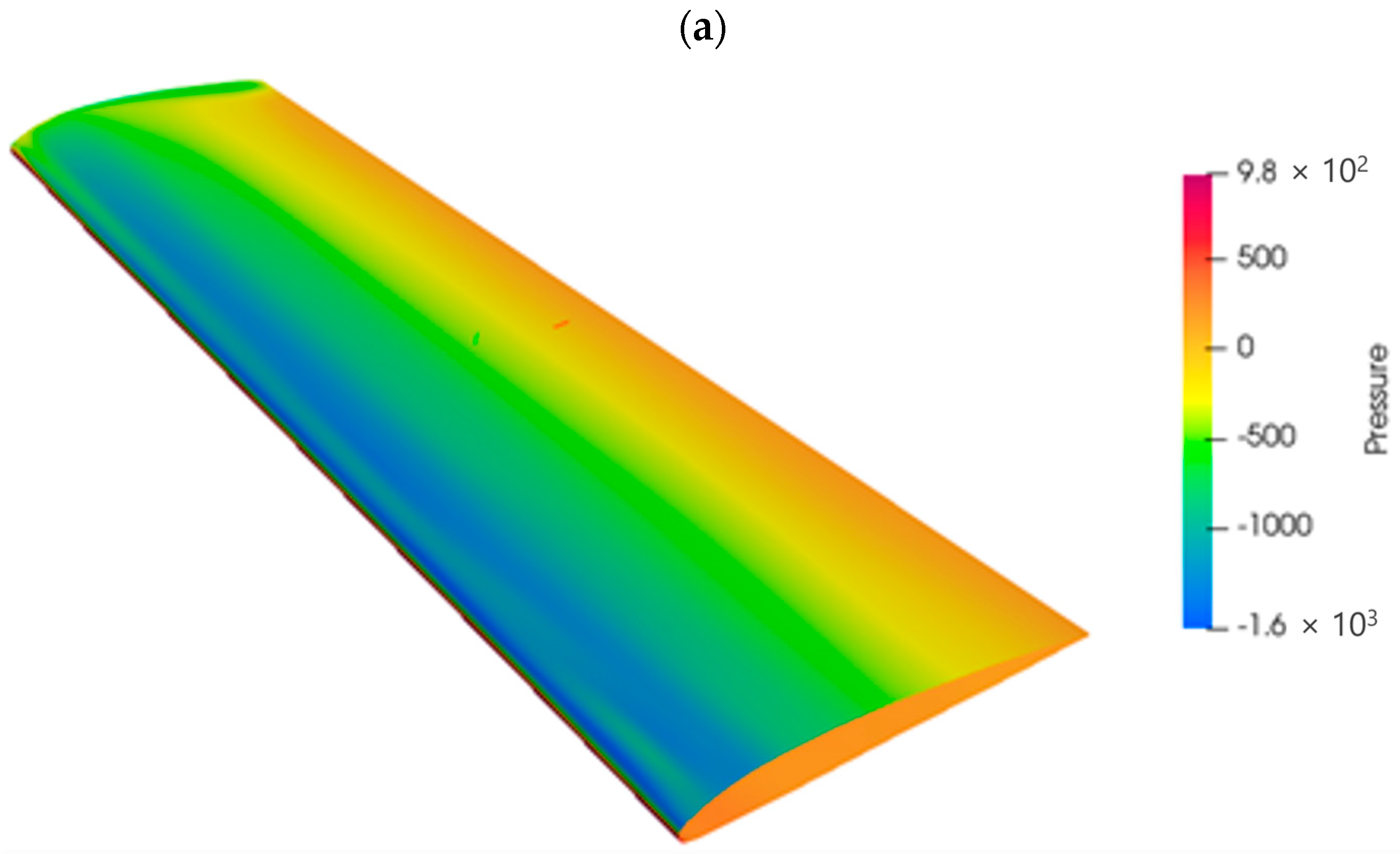
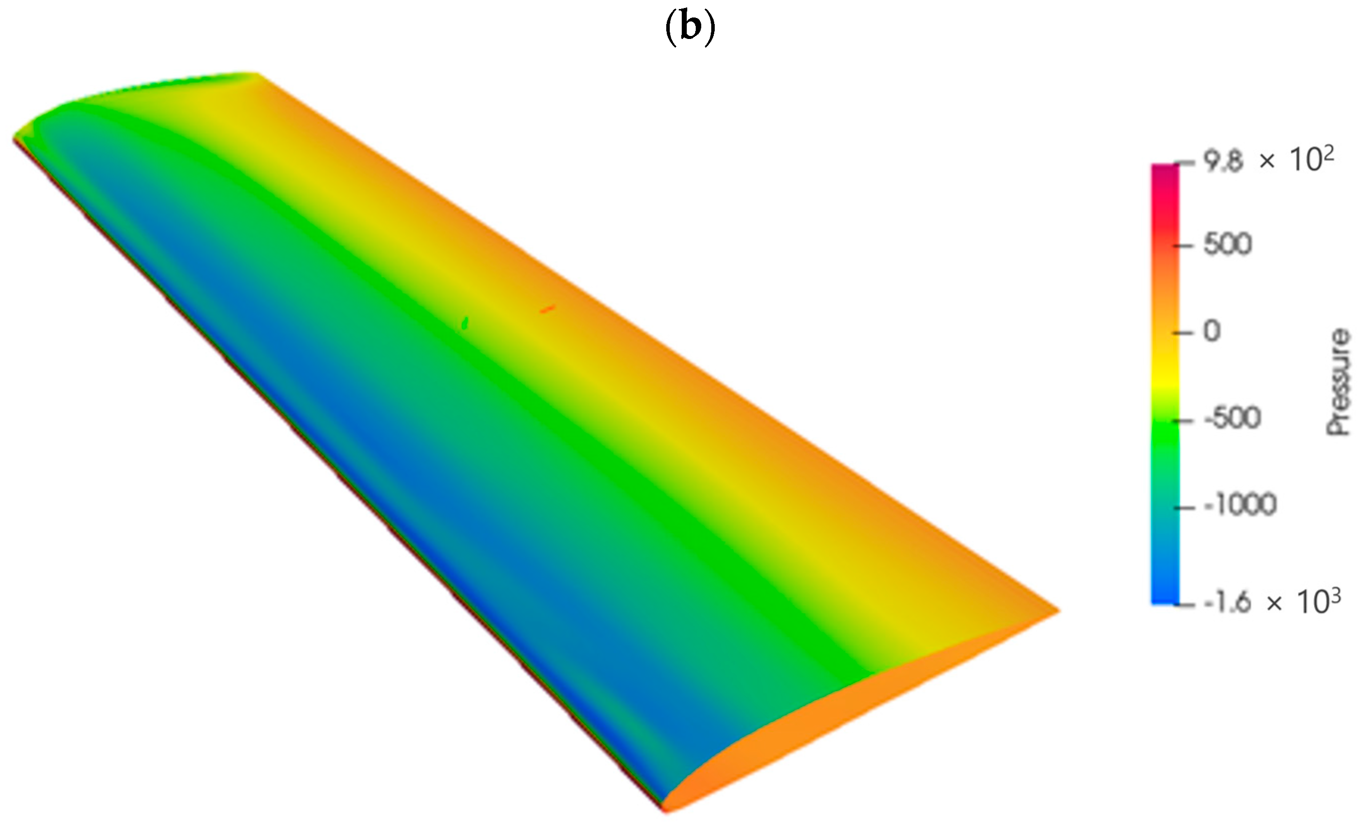
The results, particularly for the pressure field (used for mapping), were compared with those retrieved with the commercial solver ANSYS Fluent (considered the reference solver). As shown in Figure 2, a good agreement between the results is observed.


Figure 2.
Comparison of the pressure fields for the RIBES wing obtained with Fluent (a) and SU2 (b).
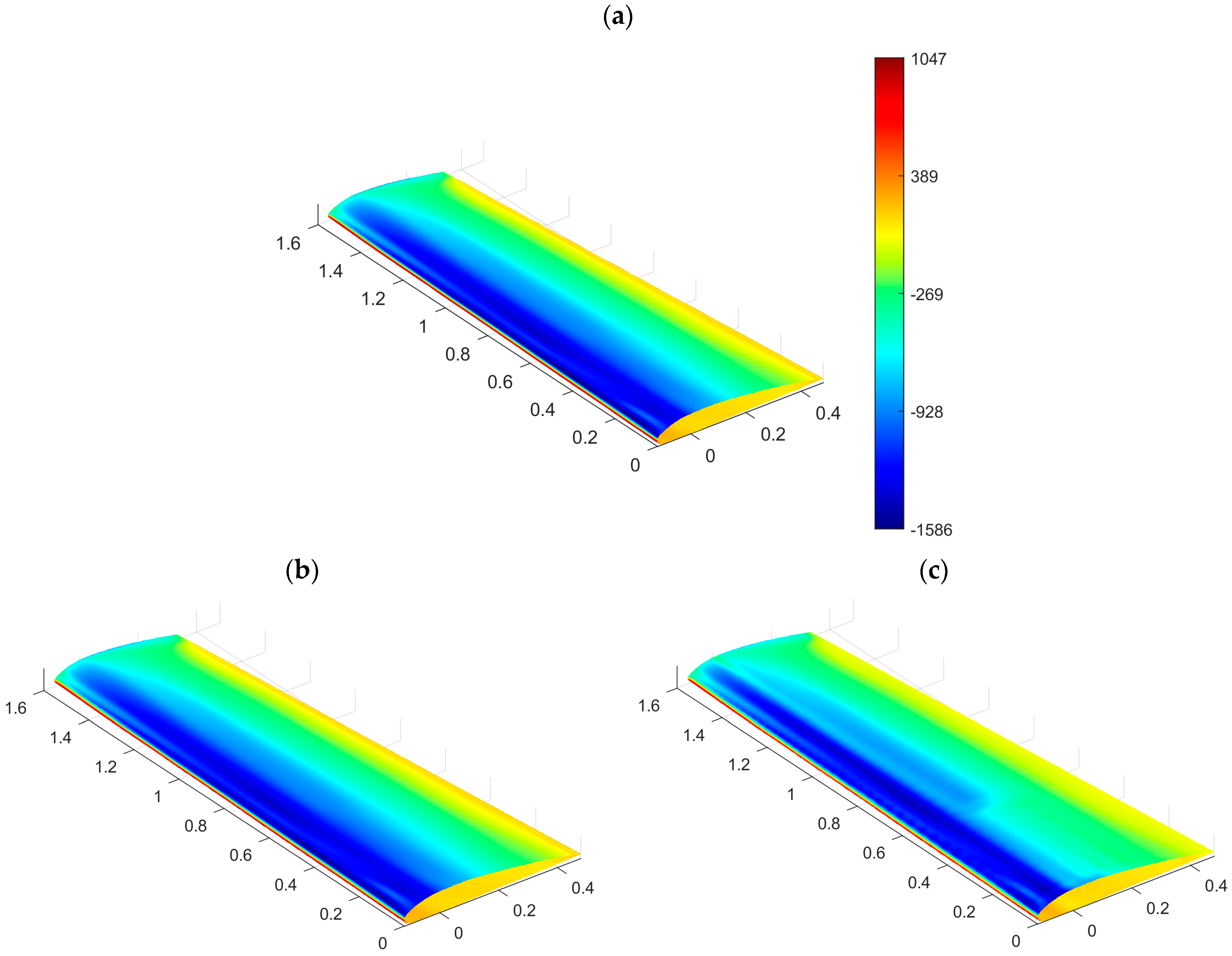
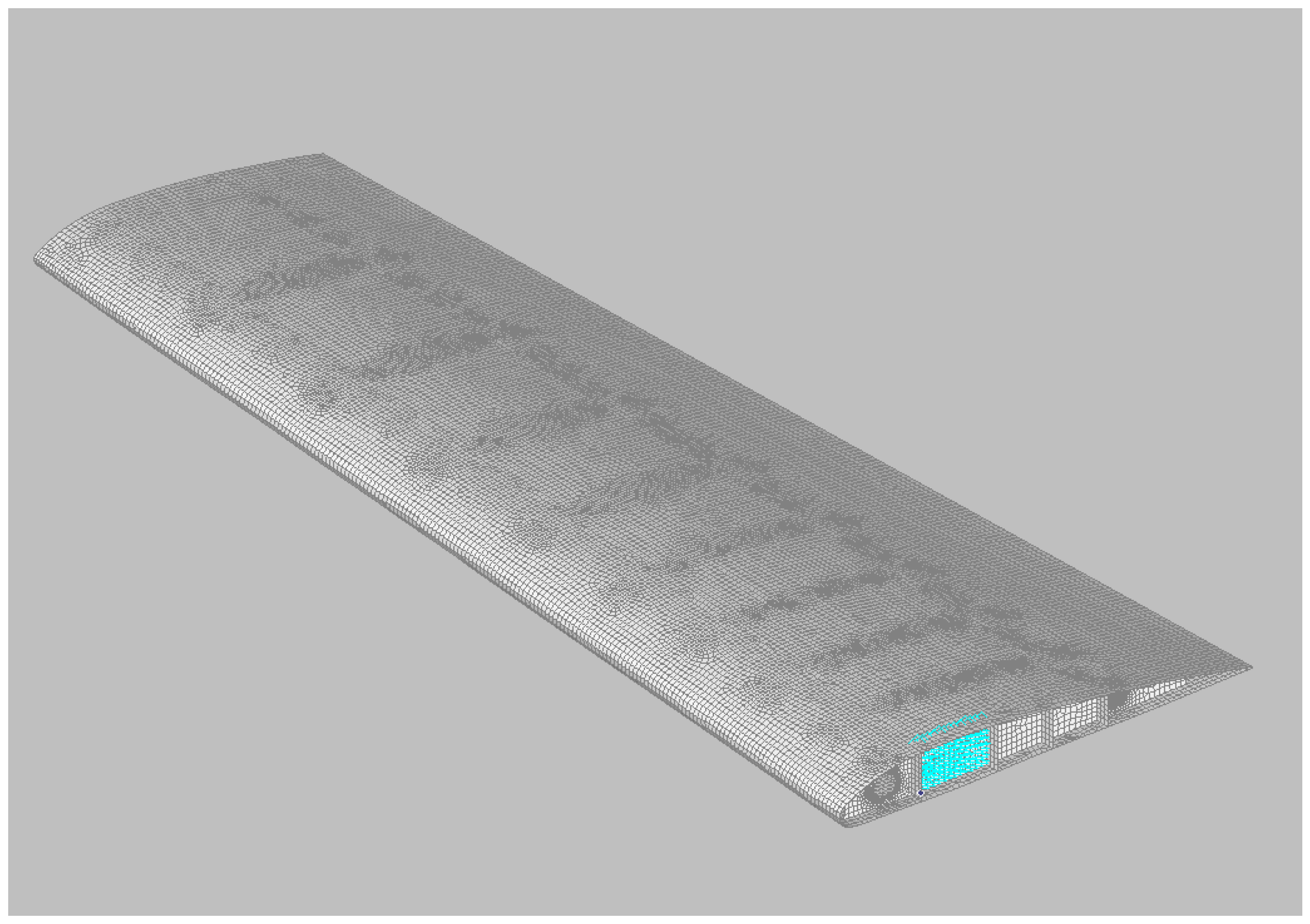
The CFD wing boundary was extracted from the whole model upon removal of the wing cap, mismatching with the CSM one, and the trailing edge (Figure 3). This last aspect occupies a tiny portion of the overall model and contains almost coincident nodes; consequently, its contribution appears irrelevant under the point of view of global balance. The resulting wing hull comprises 8673 quadrilateral patches and 8900 nodes. The CSM model incorporates a wing skin reinforced with ribs and spars. Only the mesh of the wing skin enters the mapping process, while the model retains its reinforcements for the final stress assessment. The target mesh consists of 47,082 triangular and quadrilateral elements and 45,846 nodes. The RIBES method utilizes RBF interpolation and scans the interval specified in Equation (5) to determine the optimal correction scheme for rotational balance. This second phase of the workflow represents the algorithm bottleneck, with a total computing time of 1030 s on a Dell Precision T5810 with a 3.50 GHz processor, 48 GB of RAM and 6 working cores. Figure 4 presents a triple comparison: the pressure field on the source mesh, shown above (a), and the pressure on the target domain before (result of plain RBF interpolation) and after correction, shown on the bottom left (b) and right (c), respectively. At first glance, all the represented pressure fields appear similar; anyway, solutions b and c for the target lead to widely different sets of force and moment resultants. The difference in the pressure field on the suction side is visible with the corrected pressure field, as it adjusts to the local mesh refinement. Table 5 reports the balance percentage errors for the traction field mapped with the RIBES method against the source one. A stress assessment was conducted in FEMAP, using Nastran as the solver, loading the complete CSM model with the corrected mapped field. FEMAP employs the solid potential method to model solid bodies [52], which forms the foundation of FEM formulation. The wing is made of Aluminum 2024-T3, with its mechanical properties detailed in Table 6. The material behavior was assumed to be linearly elastic and isotropic, following Hooke’s law:
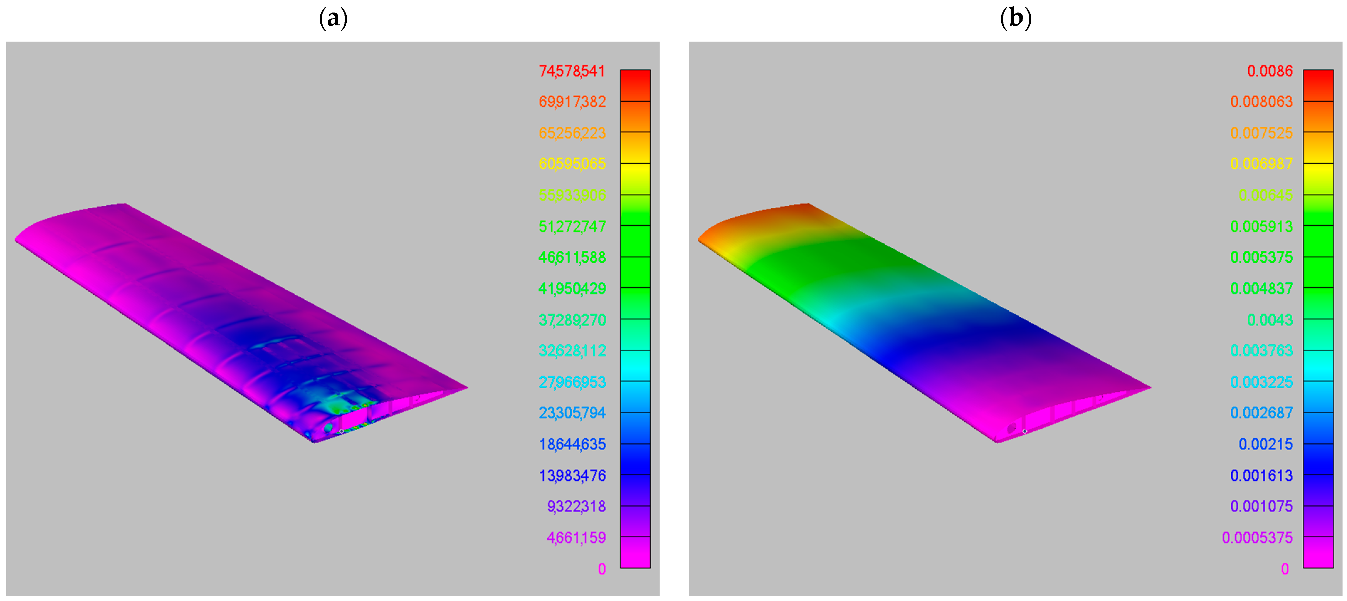
where is the vector of stress components and is the vector of strain components. The structural model was anchored at the base, simulating the attachment of the wing to the fuselage, following the scheme of a simple cantilever beam, as visible in Figure 5, where constrained nodes are marked with cyan triangles. The maximum values of Von Mises stress and vertical deflection are 69.8 MPa and 8.1 mm, respectively. Figure 6 displays stress and displacement maps resulting from the FEM analyses.

Figure 3.
CFD mesh before (a) and after (b) the removal of the wing cap and the trailing edge.

Figure 4.
Pressure field on RIBES wing: CFD source model (a), CSM target model with pressure field interpolated by plain RBF (b), CSM target model with pressure field mapped with RIBES method (c).

Table 5.
Percentage errors on global resultants, component-wise () and for vectors (). For the RIBES wing, and employing the RIBES method.

Table 6.
Mechanical properties of Aluminum 2024-T3.

Figure 5.
CSM model with fixed nodes highlighted by cyan triangles.
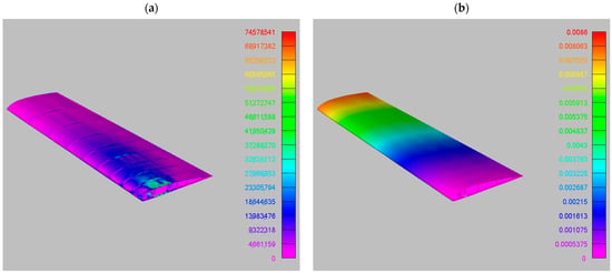
Figure 6.
FEM output for the mapped loads from the RIBES method: (a) Von Mises stress, maximum value 69.8 MPa; (b) vertical deflection, maximum value 8.1 mm.
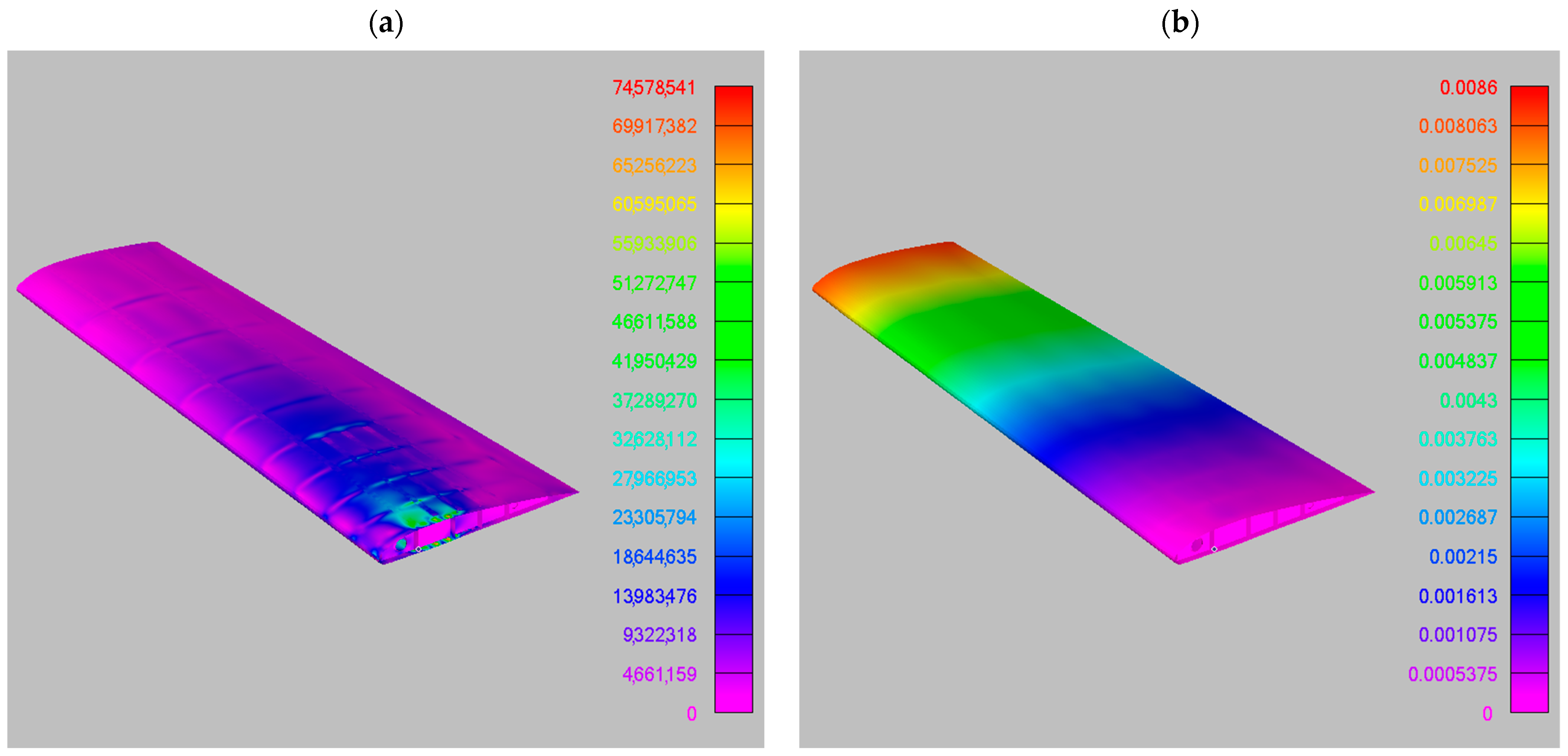
The same mapping instance was then addressed with the preCICE algorithm, again opting for the consistency-preserving option. The time required for data transfer was 9000 s. Table 7 illustrates the balance errors, while Figure 7 depicts the target pressure fields. Additionally, Figure 8 presents the results from FEM in terms of displacements and stresses, with maximum values of Von Mises stress and vertical displacements reaching 72.5 MPa and 8.25 mm, respectively.

Table 7.
Percentage errors on global resultants, component-wise () and for vectors (). For the RIBES wing, and employing the preCICE algorithm.
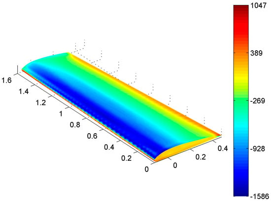
Figure 7.
Pressure field on RIBES wing CSM target model with pressure field interpolated by consistent preCICE algorithm.

Figure 8.
FEM output for the preCICE mapped loads: (a) Von Mises stress, maximum value 72.5 MPa; (b) vertical deflection, maximum value 8.25 mm.
3. Discussion
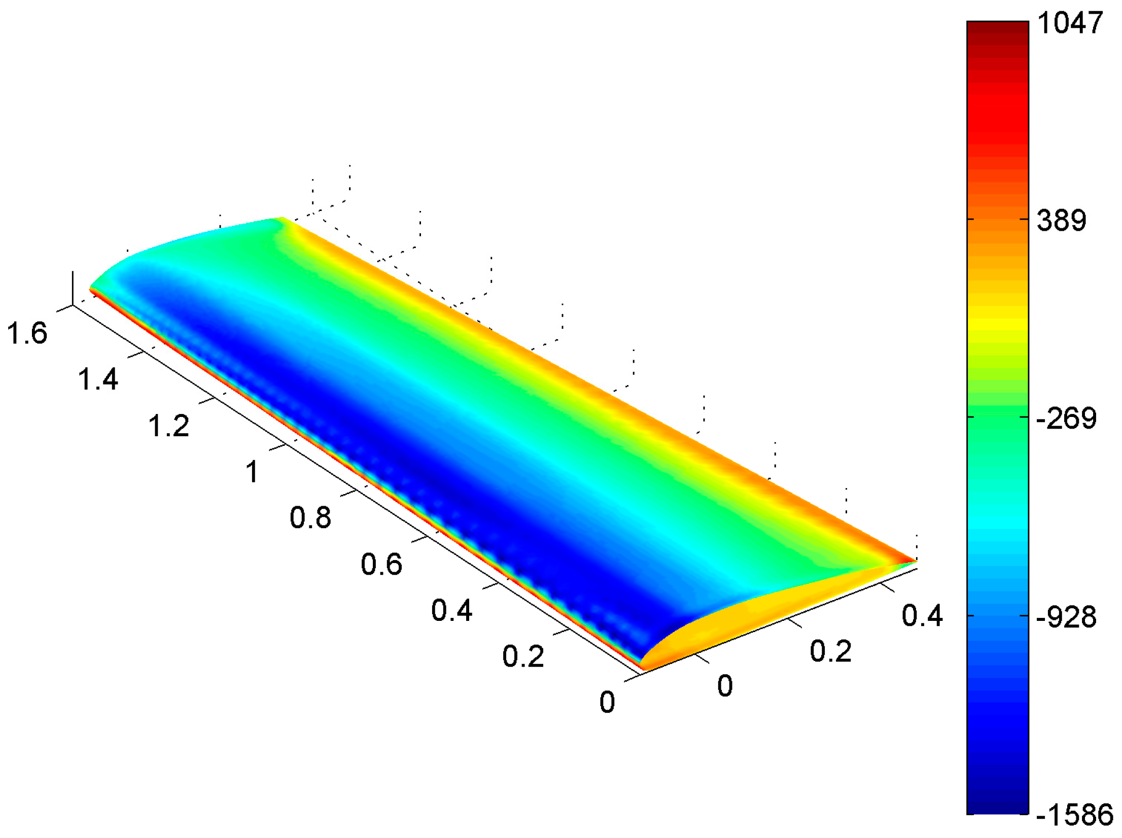
A well-designed mapping algorithm should map information across mismatching grids in a conservative manner, i.e., no data loss or alteration must occur. At the same time, it is supposed to be consistent, in the sense that a pointwise source field varying in a certain interval should keep its overall trend over the target mesh and range in-between similar bounds. Furthermore, the mapping algorithm is performant if it can complete all the above in a reasonable time and with no excessive usage of computational resources. The RIBES method attempts to meet these criteria by combining the consistency of RBF interpolation with a subsequent phase that utilizes fuzzy sets to enforce balance conservation retrospectively. Significant time savings can be achieved through the adoption of boundary decomposition methods and computational parallelization. The preCICE algorithm leaves the choice between consistency and conservation to the user, revealing a weakness in guaranteeing both simultaneously. In its conservative form, which is suitable for non-cumulative quantities, the preCICE algorithm performs a straightforward interpolation using RBFs. This method leverages the smoothness and scalability of RBFs to produce a continuous output within the same bounds as the source field. However, RBFs alone do not ensure the conservation of global quantities, such as force and moment resultants, because these depend on the model discretization and node distribution across the surface. The RIBES method tweaks the pressure field obtained from a plain RBF interpolation by accounting for local grid discretization while maintaining continuity. It employs fuzzy logic to handle granular information, such as the assignment of spotted areas to nodes. The originality of the RIBES method lies in its combination of two distinct steps aimed at different objectives, adjusting the RBFs’ interpolated pressure field minimally to achieve a satisfactory level of balance. In this study, the authors compared the RIBES method against the consistent preCICE algorithm across two distinct test scenarios. Regarding consistency, both approaches demonstrated high quality: the mapped fields closely resembled the source field, with color plots displaying similar variations across domains without significant over- or under-shoots. From a balance perspective, the RIBES method has an advantage due to its underlying mathematical formulation, which ensures translational balance. Moreover, the local action of the correction procedure leads to lower discrepancies in the rotational balance compared to the preCICE approach. Figure 9 shows the target wing skin where the difference between the two mapped pressure fields (RIBES method–preCICE algorithm) is presented, normalized by the maximum absolute value of the source pressure. It can be observed that the local pressure discrepancy is minimal over most of the wing. However, small areas on the suction side and trailing edge experience a pressure difference of about 26% of the maximum absolute value. Variations on the leading edge are due to differences in the homogeneity of the local mapped pressure: the RIBES method produces a continuous distribution, while the preCICE algorithm results in a more scattered output. Regarding performance, it is worth noting that while the RIBES method achieves considerably faster data transfer, the preCICE algorithm, in its basic form, handles the problem according to a plain serial approach. Therefore, this aspect should be excluded from the comparison since the underlying conditions differ.
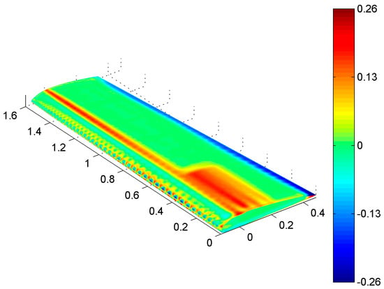
Figure 9.
Map of the difference in the mapped pressure fields (RIBES method–preCICE), normalized to the maximum absolute source pressure (1586 Pa).
As regards FEM results for the RIBES wing, Von Mises stress peaks differ by 3.87%, with maximum deflections by 1.85% between the two mapped fields. Figure 10a illustrates the difference map of Von Mises stress between the results shown in Figure 6a and Figure 8a, normalized to the maximum stress value. Figure 10b shows the normalized difference in vertical displacements between the results depicted in Figure 6b and Figure 8b. The maximum local variations in stress are approximately 10%, while the maximum local difference in deflections is around 3%. The greatest local variations in Von Mises stress occur along the longitudinal edge of the internal wing reinforcements, corresponding to the rib vertices. The stress and displacement fields largely coincide, and discrepancies in their maximum values, although noticeable, are not significant. However, it is worth noting that the model being considered is a wing mock-up with a limited wingspan and width, loaded and constrained as a cantilever. These conditions are probably not the most suitable to highlight variations in FEM output, which leads to contained differences in results despite significant differences in balance. The observed discrepancies may vary for full-scale models, with different boundary conditions or with different geometries involved. Thus, the discussed methods are valuable as precise investigation tools.
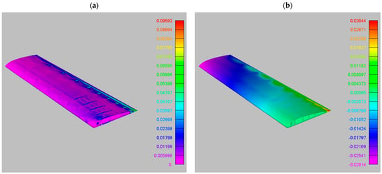
Figure 10.
Local differences between outputs from the RIBES method and the preCICE algorithm in terms of Von Mises stress (a) and vertical deflections (b), normalized to their respective maximum values.
4. Conclusions
This paper provides a comparative analysis of two load mapping techniques used to transfer data between computational fluid dynamics (CFD) and computational structural mechanics (CSM) modules in fluid–structure interaction (FSI) applications. Radial basis functions (RBFs) are key components of both algorithms, namely, the RIBES method and the one integrated into the preCICE library. These approaches were evaluated in two different scenarios: a simpler case involving the parametric geometry of the catenoid, and a practical application of the RIBES wing, utilized in the aeroelasticity experimental campaign as part of the RIBES EU project. The RIBES method exhibited higher precision in preserving balance between the source and target domains. Utilizing the mapped traction fields on the wing to individually load the structural model in FEM analyses revealed that variations in balance could impact the obtained fields to an extent that, in this specific case, proved to be noticeable yet not significant.
Author Contributions
Conceptualization, A.C., A.L. and C.G.; methodology, A.C.; software, A.C., A.L. and C.G.; validation, A.C. and C.G.; formal analysis, A.C. and C.G.; investigation, A.C.; resources, A.C., A.L. and C.G.; data curation, A.C.; writing—original draft preparation, A.C.; writing—review and editing, A.C. and A.L.; visualization, A.C. All authors have read and agreed to the published version of the manuscript.
Funding
This research received no external funding.
Data Availability Statement
Part of the original data presented in this study are openly available in the RIBES database at http://ribes-project.eu/, accessed on 27 April 2024.
Conflicts of Interest
The authors declare no conflicts of interest.
References
- Hsu, M.C.; Bazilevs, Y. Fluid-structure interaction modelling of wind turbines: Simulating the full machine. Comput. Mech. 2012, 50, 821–833. [Google Scholar] [CrossRef]
- Wuchner, R.; Kupzok, A.; Bletzinger, K.U. A framework for stabilized partitioned analysis of thin-membrane-wind interaction. Int. J. Numer. Methods Fluids 2007, 54, 945–963. [Google Scholar] [CrossRef]
- Stein, K.; Benney, R.; Kalro, V.; Johnson, A.; Tezduyar, T.; Stein, K.; Benney, R.; Kalro, V.; Johnson, A.; Tezduyar, T. Parallel computation of parachute fluid-structure interactions. In Proceedings of the 14th Aerodynamic Decelerator Systems Technology Conference, San Francisco, CA, USA, 3–5 June 1997. [Google Scholar]
- Farhat, C.; Van der Zee, K.G.; Geuzaine, P. Provably second-order time-accurate loosely-coupled solution algorithms for transient nonlinear computational aeroelasticity. Comput. Methods Appl. Mech. Eng. 2006, 195, 1973–2001. [Google Scholar] [CrossRef]
- Keyes, D.E.; McInnes, L.C.; Woodward, C.; Gropp, W.; Myra, E.; Pernice, M.; Bell, J.; Brown, J.; Clo, A.; Connors, J.; et al. Multiphysics simulations: Challenges and opportunities. Int. J. High. Perform. Comput. Appl. 2013, 27, 4–83. [Google Scholar] [CrossRef]
- Michler, C.; Hulshoff, S.J.; Van Brummelen, E.H.; De Borst, R. A monolithic approach to fluid–structure interaction. Comput. Fluids 2004, 33, 839–848. [Google Scholar] [CrossRef]
- Wong, K.K.; Thavornpattanapong, P.; Cheung, S.C.; Tu, J. Numerical stability of partitioned approach in fluid-structure interaction for a deformable thin-walled vessel. Comput. Math. Methods Med. 2013, 2013, 638519. [Google Scholar] [CrossRef]
- Wang, T.; Wüchner, R.; Sicklinger, S.; Bletzinger, K.U. Assessment and improvement of mapping algorithms for non-matching meshes and geometries in computational FSI. Comput. Mech. 2016, 57, 793–816. [Google Scholar] [CrossRef]
- Cebral, J.R.; Lohner, R. Conservative load projection and tracking for fluid-structure problems. AIAA J. 1997, 35, 687–692. [Google Scholar] [CrossRef]
- Jiao, X.; Heath, M.T. Common-refinement-based data transfer between non-matching meshes in multiphysics simulations. Int. J. Numer. Methods Eng. 2004, 61, 2402–2427. [Google Scholar] [CrossRef]
- Puso, M.A. A 3D mortar method for solid mechanics. Int. J. Numer. Methods Eng. 2004, 59, 315–336. [Google Scholar] [CrossRef]
- Dukowicz, J.K. Conservative rezoning (remapping) for general quadrilateral meshes. J. Comput. Phys. 1984, 54, 411–424. [Google Scholar] [CrossRef]
- Ramshaw, J.D. Conservative rezoning algorithm for generalized two-dimensional meshes. J. Comput. Phys. 1985, 59, 193–199. [Google Scholar] [CrossRef]
- Grandy, J. Conservative remapping and region overlays by intersecting arbitrary polyhedra. J. Comput. Phys. 1999, 148, 433–466. [Google Scholar] [CrossRef]
- Jones, P.W. First-and second-order conservative remapping schemes for grids in spherical coordinates. Mon. Weather Rev. 1999, 127, 2204–2210. [Google Scholar] [CrossRef]
- Hou, G.; Satyanarayana, A. Analytical sensitivity analysis of a static aeroelastic wing. In Proceedings of the 8th Symposium on Multidisciplinary Analysis and Optimization, Long Beach, CA, USA, 6–8 September 2000; p. 4824. [Google Scholar]
- Hou, G.; Wang, J.; Layton, A. Numerical methods for fluid-structure interaction—A review. Commun. Comput. Phys. 2012, 12, 337–377. [Google Scholar] [CrossRef]
- Huang, H.; Cui, C.; Cheng, L.; Liu, Q.; Wang, J. Grid interpolation algorithm based on nearest neighbor fast search. Earth Sci. Inform. 2012, 5, 181–187. [Google Scholar] [CrossRef]
- Silva, G.H.; Le Riche, R.; Molimard, J.; Vautrin, A. Exact and efficient interpolation using finite elements shape functions. Eur. J. Comput. Mech. 2009, 18, 307–331. [Google Scholar] [CrossRef]
- Gasca, M.; Sauer, T. Polynomial interpolation in several variables. Adv. Comput. Math. 2000, 12, 377–410. [Google Scholar] [CrossRef]
- Smith, M.; Cesnik, C.; Hodges, D.; Moran, K. An evaluation of computational algorithms to interface between CFD and CSD methodologies. In Proceedings of the 37th Structure, Structural Dynamics and Materials Conference, Salt Lake City, UT, USA, 15–17 April 1997. [Google Scholar]
- Franke, R. Scattered data interpolation: Tests of some methods. Math. Comput. 1982, 38, 181–200. [Google Scholar]
- Biancolini, M.E.; Chiappa, A.; Giorgetti, F.; Groth, C.; Cella, U.; Salvini, P. A balanced load mapping method based on radial basis functions and fuzzy sets. Int. J. Numer. Methods Eng. 2018, 115, 1411–1429. [Google Scholar] [CrossRef]
- preCICE v2: A Sustainable and User-Friendly Coupling Library. Available online: https://open-research-europe.ec.europa.eu/articles/2-51/v2 (accessed on 30 March 2023).
- Cella, U.; Della Vecchia, P.; Groth, C.; Porziani, S.; Chiappa, A.; Giorgetti, F.; Nicolosi, F.; Biancolini, M.E. Wind tunnel model design and aeroelastic measurements of the ribes wing. J. Aerosp. Eng. 2021, 34, 04020109. [Google Scholar] [CrossRef]
- Biancolini, M.E.; Groth, C.; Porziani, S.; Chiappa, A.; Giorgetti, F.; Nicolosi, F.; Cella, U. Validation of structural modeling for realistic wing topologies involved in fsi analyses: Ribes test case. J. Aerosp. Eng. 2021, 34, 04020110. [Google Scholar] [CrossRef]
- Fasshauer, G.E. Meshfree Approximation Methods with MATLAB; World Scientific: Singapore, 2007; Volume 6. [Google Scholar]
- Buhmann, M.D. Radial Basis Functions. Acta Numer. 2000, 9, 1–38. [Google Scholar] [CrossRef]
- Biancolini, M.E. Fast Radial Basis Functions for Engineering Applications; Springer International Publishing: Berlin/Heidelberg, Germany, 2017. [Google Scholar]
- Boyd, J.P.; Gildersleeve, K.W. Numerical experiments on the condition number of the interpolation matrices for radial basis functions. Appl. Numer. Math. 2011, 61, 443–459. [Google Scholar] [CrossRef]
- Babuška, I.; Melenk, J.M. The partition of unity method. Int. J. Numer. Methods Eng. 1997, 40, 727–758. [Google Scholar] [CrossRef]
- Haykin, S. Neural Networks: A Comprehensive Foundation; Prentice Hall PTR: Hoboken, NJ, USA, 1998. [Google Scholar]
- Casciola, G.; Lazzaro, D.; Montefusco, L.B.; Morigi, S. Shape preserving surface reconstruction using locally anisotropic radial basis function interpolants. Comput. Math. Appl. 2006, 51, 1185–1198. [Google Scholar] [CrossRef]
- Biancolini, M.E. Mesh morphing and smoothing by means of radial basis functions (RBF): A practical example using fluent and RBF morph. In Handbook of Research on Computational Science and Engineering: Theory and Practice; IGI Global: Hershey, PA, USA, 2012; pp. 347–380. [Google Scholar]
- De Boer, A.; Van der Schoot, M.S.; Bijl, H. Mesh deformation based on radial basis function interpolation. Comput. Struct. 2007, 85, 784–795. [Google Scholar] [CrossRef]
- Biancolini, M.E.; Salvini, P. Radial Basis Functions for the image analysis of deformations. In Proceedings of the CompIMAGE, Rome, Italy, 5–9 September 2012. [Google Scholar]
- Groth, C.; Chiappa, A.; Porziani, S.; Biancolini, M.E.; Marotta, E.; Salvini, P. A post-processing method based on radial basis functions for the fast retrieval of the strain field in digital image correlation methods. Materials 2022, 15, 7936. [Google Scholar] [CrossRef] [PubMed]
- Groth, C.; Chiappa, A.; Porziani, S.; Salvini, P.; Biancolini, M.E. An RBF meshless approach to evaluate strain due to large displacements in flexible printed circuit boards. Micromachines 2022, 13, 1163. [Google Scholar] [CrossRef]
- Kardampiki, E.; Vignali, E.; Haxhiademi, D.; Federici, D.; Ferrante, E.; Porziani, S.; Chiappa, A.; Groth, C.; Cioffi, M.; Biancolini, M.E.; et al. The hemodynamic effect of modified blalock–taussig shunt morphologies: A computational analysis based on reduced order modeling. Electronics 2022, 11, 1930. [Google Scholar] [CrossRef]
- Groth, C.; Chiappa, A.; Biancolini, M.E. Shape optimization using structural adjoint and RBF mesh morphing. Procedia Struct. Integr. 2018, 8, 379–389. [Google Scholar] [CrossRef]
- Valentini, P.P.; Biancolini, M.E. Interactive sculpting using augmented-reality, mesh morphing, and force feedback: Force-feedback capabilities in an augmented reality environment. IEEE Consum. Electron. Mag. 2018, 7, 83–90. [Google Scholar] [CrossRef]
- Chiappa, A.; Salvini, P.; Brutti, C.; Biancolini, M.E. Upscaling 2D finite element analysis stress results using radial basis functions. Comput. Struct. 2019, 220, 131–143. [Google Scholar] [CrossRef]
- Chiappa, A.; Groth, C.; Biancolini, M.E. A two-scale RBF meshless method for the interface stress retrieval in simply bended and torqued long-fibres laminates. Compos. Struct. 2023, 306, 116600. [Google Scholar] [CrossRef]
- Zadeh, L.A. Fuzzy sets. Inf. Control 1965, 8, 338–353. [Google Scholar] [CrossRef]
- Yates, E.C. AGARD standard aeroelastic configurations for dynamic response, I-wing 445.6. In Technical Memorandum (TM); NASA Langley Research Center: Hampton, VA, USA, 1988. [Google Scholar]
- Ballmann, J. Experimental analysis of high Reynolds number structural dynamics in ETW. In Proceedings of the 46th AIAA Aerospace Sciences Meeting and Exhibit, Reno, NV, USA, 7–10 January 2008; p. 841. [Google Scholar]
- Kuzmina, S.I.; Ishmuratov, F.; Zichenkov, M.; Chedrik, V. Integrated numerical and experimental investigations of the Active/Passive Aeroelastic concepts on the European Research Aeroelastic Model (EuRAM). ASD J. 2011, 2, 31–51. [Google Scholar] [CrossRef]
- Laflin, K.R.; Klausmeyer, S.M.; Zickuhr, T.; Vassberg, J.C.; Wahls, R.A.; Morrison, J.H.; Brodersen, O.P.; Rakowitz, M.E.; Tinoco, E.N.; Godard, J.L. Data summary from second AIAA computational fluid dynamics drag prediction workshop. J. Aircr. 2005, 42, 1165–1178. [Google Scholar] [CrossRef]
- Turek, S.; Hron, J. Proposal for numerical benchmarking of fluid-structure interaction between an elastic object and laminar incompressible flow. In Fluid-Structure Interaction, 1st ed.; Hans-Joachim Bungartz, H.J., Michael Schäfer, M., Eds.; Spinger: Berlin/Heidelberg, Germany, 2006; pp. 371–385. [Google Scholar]
- RIBES Project. Available online: http://ribes-project.eu/ (accessed on 28 March 2024).
- Landau, L.D.; Lifshitz, E.M. Fluid Mechanics: Landau and Lifshitz: Course of Theoretical Physics, 2nd ed.; Pergamon Press: Oxford, UK, 1987; Volume 6. [Google Scholar]
- Hughes, T.J. The Finite Element Method: Linear Static and Dynamic Finite Element Analysis; Dover Publications, Inc.: Mineola, NY, USA, 2012. [Google Scholar]
Disclaimer/Publisher’s Note: The statements, opinions and data contained in all publications are solely those of the individual author(s) and contributor(s) and not of MDPI and/or the editor(s). MDPI and/or the editor(s) disclaim responsibility for any injury to people or property resulting from any ideas, methods, instructions or products referred to in the content. |
© 2024 by the authors. Licensee MDPI, Basel, Switzerland. This article is an open access article distributed under the terms and conditions of the Creative Commons Attribution (CC BY) license (https://creativecommons.org/licenses/by/4.0/).

