Control of Aerodynamic Characteristics of Thick Airfoils at Low Reynolds Numbers Using Methods of Boundary Layer Control

Abstract

The article explores flow behavior around thick airfoils at low Reynolds numbers and the potential application of energy methods to manipulate the flow field for increased lift and reduced drag. The study relies on a set of propulsion airfoils calculated using a combined approach of solving the inverse problem of aerodynamics and applying stochastic global optimization methods. The calculations consider the transition from laminar to turbulent flow regimes, which significantly affects lift and airfoil drag. The suitability of different turbulence models for airfoil modeling in low Reynolds numbers is discussed, and numerical simulation results determine the lift coefficient dependence on angle of attack and the optimal air flow rate taken from the airfoil surface for each angle of attack. The accuracy of different turbulence models is analyzed by comparing numerical simulation results to physical experiment data.

1. Introduction

Energy methods, which were widely used in the early development of short-takeoff-and-landing transport aircraft [1,2,3], are used to achieve break-free streamlining of large-height airfoils. More recently, these methods have been implemented to resolve challenges related to the seamless integration of propulsion systems with aircraft airframes as well as the utilization of engines to promote flow laminarization and boundary layer usage near aerodynamic surfaces [4,5].

Integrated propulsion system design combines the structural elements of an engine and aerodynamic surfaces to create lift force in one element. This design improves the weight capacity of the aircraft due to the use of the fuselage to generate lift, so many promising aircraft are being developed with the realization of this design scheme. The low flight speeds, large internal volume, height of the aerodynamic profile in the cross-section, small wing elongation, significant influence of vortex and breakaway effects are characteristic features pertinent to such aircraft. These attributes, coupled with laminarization technology, give rise to a highly intricate spatial flow structure. Designing the aircraft control system and analyzing it holistically pose daunting challenges. Thus, an important issue is to develop and form high-precision applied numerical methods to calculate the aerodynamics of such systems accurately [6].

Placing the air intake of the integrated propulsion system at the critical upper point of the profile generates a continuous laminar flow in the profile section, resulting in high aerodynamic quality. The profile section beyond the air intake, upon air intake from the upper surface, produces thrust akin to a nozzle. The creation of thrust force as a result of air intake operation is a topic tackled in contemporary scientific and technical literature [7].

Thick airfoils with air extraction from the upper surface have been researched extensively utilizing the mathematical model of the vortex cell [8]. The extraction of air from the cell and its release through a slot nozzle in the profile’s trailing edge resulted in a good aerodynamic quality even for very large relative profile thicknesses. Meanwhile, achieving the conditions of uninterrupted aerodynamic surface flow presents a challenging task, as it necessitates providing the necessary parameters for the injected flow. Meeting the requirements for in-channel thrusters to ensure proper operation may be unacceptable within the context of the propulsive wing design problem.

The traditional method of aerodynamic design involves increasing wing span to maximize the lift-to-thrust ratio and transportation efficiency [9]. The implementation of an adjustable wing presents a potential solution for enhancing the takeoff and landing performance of aircraft. By altering the curvature of the airfoil, there is an opportunity to manipulate the pressure distribution over the wing and subsequently regulate aerodynamic forces and moments. The application of suction in the boundary layer enables the modification of the flow pattern around a thick aerodynamic wing from a separated state to a practically continuous one. This transformation results in an elevation of the lift force and lift-to-drag ratio. The calculation of the drag coefficient takes into consideration supplementary drag attributed to energy expenditures connected with air suction.

The advancement of propulsive airfoil technology results in the emergence of novel aircraft lift surface configurations [8] (Griffith–Goldschmied airfoil concept). The wing’s trailing edge discharges air bled from the upper surface, producing supplementary thrust. Due to the extraction of air from the airfoil’s upper critical point and its release through the trailing edge, the wing’s super-circulation is actively regulated [10]. Without air extraction, such airfoils have poor streamlining, while with the required air flow through the internal channel, the tail section of the airfoil generates thrust. The procedure for air extraction is technically executed through a transverse (tangential) fan (crossflow fan or CFF) [11,12,13]. By altering the fan blade rotation speed, separation of the boundary layer can be avoided [4].

The modification of existing airfoils and the design of new ones to enhance their aerodynamic properties have been extensively analyzed in numerous studies [1,2,3]. Several types of airfoils that incorporate internal channels and energy principles for lift augmentation and thrust generation by extracting air from a critical point on the wing’s trailing edge have been developed. Air is drawn from the upper surface of a jet-slotted wing through slots located in the middle part of the airfoil and at the trailing edge. It is then blown tangentially onto the upper surface of the wing through a slot located at the leading edge. The wing’s circulation and lift increase due to the presence of an internal channel that allows air to flow in the direction of flight [14].

Considerable attention has been devoted in the literature to regulating the airflow around airfoils by forming deliberate large-scale vortex structures [15]. By utilizing vortex cells, it becomes feasible to alter the flow structure and stabilize it, giving it a non-separated character and improving the aerodynamic features significantly [16]. Vortex cells are curvilinear cavities found in the contours of bodies. To increase the flow circulating in them, a distributed or concentrated suction (slotted) or boundary movement such as the rotation of the central body is employed [17]. Technical abbreviations will be explained upon first usage. The flow in the vortex cell (cavity) may become unstable under certain conditions [18], and boundary layer suction [19] is used to enhance the efficiency of the vortex cell.

Placing a vortex cell on a semicircular airfoil’s surface, accompanied by slit suction and ejection into the nearby wake, results in reconstructing the low-velocity flow’s unsteady separation pattern around the airfoil [20]. The separation point of the flow shifts to the airfoil’s trailing edge, and the lift changes from ultra-low negative to positive, while the drag is decreased by half. The static pressure reduces by two to three times on the upper surface and doubles on the lower surface. Moreover, the level of pressure fluctuations decreases significantly. Implementing longitudinal slotted cuts facilitates a flow pattern restructuring around the body, resulting in a decrease or elimination of separation zones and a noteworthy improvement in the integral characteristics [21].

Passive vortex cells without suction are ineffective as the separated flow intensity is low and the effect on the external flow is weak. Empirically, the aerodynamic characteristics of the airfoil with vortex cells are the same as those without them. Vortex cell usage creates multiple technological requests concerning flight dynamics and control, integrated aerodynamic configurations and power plants of aircraft and design methods.

The airfoils located in the tail portion of the propulsion system comprise a component that functions as a nozzle contour and propels the system by extracting air from the surface [22]. The engine generates thrust by moving air from the surface and pumping it through channels. As a result, the pressure on the traction area of the wing increases, resulting in an increase in thrust. The main characteristic of propulsion airfoils is their capacity for impeding separation flow, thus decreasing drag, elevating lift and enhancing the lift-to-drag ratio at reasonable energy expenditures.

This study examines the challenge of devising high-lift airfoils through means of energy with the aim of augmenting lift force. A mathematical modeling method is developed to simulate the flow around airfoils, using the inverse problem of aerodynamics to solve for known flow properties while accounting for the laminar-turbulent transition. Geometrical modeling of airfoil shapes is completed through the target function of aerodynamic quality, which represents the lift force to drag force ratio. The precision of different turbulence models is compared in their application to the low Reynolds number airflow around a model airfoil. The relationship between the lift properties of airfoils and the air flow rates taken from their surface is analyed. The potential use of propulsion airfoils in the designs of the wings and fuselages of unmanned aerial vehicles is considered.

2. Choice of Airfoil

At low Reynolds numbers, the airfoils shown in Figure 1 have wide practical application. The E387 airfoil, with a flat surface adjacent to the trailing edge, provides fairly smooth pressure recovery. The FX63-137 and M06-13-12 airfoils have convex and concave surfaces adjacent to the trailing edge, respectively, but they have different aerodynamic characteristics. Unlike the concave surface, the convex surface of the airfoil makes it possible to provide high (negative) moments and smooth changes in aerodynamic characteristics when the flow is stalled from the rear of the airfoil. A comparison of the aerodynamic characteristics of the given airfoils is given in [23] for Reynolds numbers up to $\mathrm{Re}=2\times {10}^5$.

The evolution of the ideas of vortex cells (Glauert vortex cell) has led to the concept of a propulsive wing in which air is drawn in by a transverse fan (Figure 2). The use of traditional axial fans for flow control is not suitable because axial fans are sensitive to flow irregularities within the boundary layer and do not work well at high back pressure [24]. When the pressure drop across the fan is more than 1.15, the efficiency drops sharply, and when air is extracted from the airfoil surface, pressure drops of 1.5–2 and higher must be realized. Boundary layer air extraction with CFF provides laminar flow on the upper surface, which reduces frictional drag. Ejection of the air extracted from the surface through a slotted nozzle eliminates the vortex wake effect behind the wing. The increased pressure in the section of the airfoil from the slot to the blowing nozzle creates positive thrust.

The CFF efficiency reaches about 80%, which is lower than that of axial fans, but this is compensated by the convenience of the design, less sensitivity to flow inhomogeneity in the boundary layer, and large back pressure [13]. When the boundary layer is blown off, air can be extracted from the high-pressure region at the bottom of the wing, and the CFF will play the role of an energy flap [25].

3. Simulation of Flowfield

One stage in the numerical study of advanced aircraft’s aerodynamic characteristics is conducting a comparative analysis of results obtained with various semi-empirical turbulence models. The accuracy of each turbulence model is typically assessed through problem solving involving low-intensity turbulent eddies and separated flows [26].

The SST (Shear-Stress Transport) model, proposed by Menter in 1993 [27], and the Menter model for shear stress transport, proposed in 2003 [28], are popularly used for separated flow modeling. The SST model simplifies two turbulence models: the k–$\epsilon$ model applied to the far-off wall shear flow region and the k–$\omega$ model used in the near-wall region. The SST model offers significant benefits compared to the RNG and realizable versions from the k–$\epsilon$ family of models. Additionally, it outperforms the Spalart–Allmaras eddy viscosity model, which uses either the vorticity model or the modulus of the strain rate tensor to compute eddy viscosity as well as the V2F four-parameter model [29].

The flow around the airfoils of such a wing occurs at low Reynolds numbers ($\mathrm{Re}<5\times {10}^5$). At such Reynolds numbers, a laminar–turbulent transition may occur in the vicinity of the airfoils, which is accompanied by flow separation, an abrupt change in the aerodynamic characteristics of the airfoil, and deterioration in flight performance. With the Reynolds number $\mathrm{Re}={10}^5$, the recirculation zone occupies approximately 20–30% of the airfoil length [30]. A comparison of aerodynamic characteristics of different airfoils is given in [23,31]. A catalog of high-carrying airfoils for low flight speeds is constructed in [31] using the inverse multi-point method of conformal mappings.

The airfoil flow occurs at low Reynolds numbers ($\mathrm{Re}<5\times {10}^5$), leading to a laminar–turbulent transition and flow separation in the airfoil surface vicinity. These changes result in an abrupt shift in the airfoil’s aerodynamic characteristics and a decrease in flight performance. At $\mathrm{Re}={10}^5$, approximately 20–30% of the airfoil length is occupied by the recirculation zone [30]. A comparison of aerodynamic characteristics among various airfoils is presented in [23,31]. In [31], a catalog of airfoils that provide high lift at low flight speeds is created using the inverse multi-point method of conformal mappings.

One issue with airfoil modeling at low Reynolds numbers is the extensive laminar boundary layer region [32]. Many semi-empirical turbulence models are unreliable in predicting the transition from laminar to turbulent flow [33,34], as they significantly underestimate the intensity of separated flow by predicting a false eddy viscosity field. The available empirical models, which are based on the processing of physical experimental data, relate the critical Reynolds number of the transition to characteristics of the boundary layer such as the pressure gradient and the level of turbulence. The transition occurs in the section of the boundary layer where the local Reynolds number surpasses the critical value.

Once the boundary layer reaches a certain thickness, instability arises, leading to the formation of Tollmien–Schlichting waves. The amplitude of these waves increases exponentially, following the dependence equation of $A\sim e^N$. Assuming no external disturbances are present, the transition starts at $N=8$ and concludes at $N=11$. Generalization of the $e^N$ method to three-dimensional problems is complicated due to its basis on concepts of a two-dimensional boundary layer [35].

In external flow problems, achieving satisfactory accuracy within a wide range of angles of attack and Reynolds numbers is not possible with conventional turbulence models [36]. Several semi-empirical turbulence models consider the possibility of a laminar–turbulent transition [37]. The $\gamma$–${\mathrm{Re}}_{\theta t}$ model utilizes external empirical correlations to initiate a laminar–turbulent transition at critical local near-wall flow quantities [38,39]. The transfer equation for the intermittency parameter and the critical Reynolds number [40] is also incorporated with the equations of the SST model. About ten empirical correlations and a dozen and a half constants are necessary for closing the equations. The numerical simulations of both external and internal turbulent separated flows demonstrate the superiority of the $\gamma$–${\mathrm{Re}}_{\theta t}$ model when compared to other semi-empirical turbulence models [37,41].

4. Mathematical Model

The implementation of special wing airfoils enables the creation of a laminar flow regime in the boundary layer, leading to an improved lift-to-drag ratio. Calculating the friction forces on the aerodynamic surface relies heavily on the state of the boundary layer, further highlighting the need for accurate calculation methods when designing laminarized airfoils to determine the position of the laminar–turbulent transition.

To address the challenge related to the two-dimensional turbulent flow of viscous incompressible fluid around an airfoil, a mathematical model based on the solution of the Reynolds-averaged Navier–Stokes (RANS) equations is used. The models were utilized to conclude the RANS encompassing the Spalart–Allmaras model (SA), k–$\omega$ SST (SST model) and its varied alterations such as $\gamma$–SST and the SST model altered for low Reynolds numbers.

The model consists of four differential equations: a transport equation for turbulent kinetic energy, a transport equation for the specific dissipation rate of turbulent energy, a transport equation for intermittency, and a transport equation for the Reynolds number that corresponds to the onset of the laminar–turbulent transition.

The equations governing the kinetic energy of turbulence and its dissipation rate take the following form

$$\begin{array}{cc}\hfill & \frac{𝜕\left(\rho k\right)}{𝜕t}+\frac{𝜕\left(\rho v_{j}k\right)}{𝜕x_j}=\frac{𝜕}{𝜕x_j}\left[\left(\mu +{\sigma }_k{\mu }_t\right)\frac{𝜕k}{𝜕x_j}\right]+P_k-D_k;\hfill \end{array}$$

(1)

$$\begin{array}{cc}\hfill & \frac{𝜕\left(\rho \omega \right)}{𝜕t}+\frac{𝜕\left(\rho v_j\omega \right)}{𝜕x_j}=\frac{𝜕}{𝜕x_j}\left[\left(\mu +{\sigma }_{\omega }{\mu }_t\right)\frac{𝜕\omega }{𝜕x_j}\right]+2(1-F_1)\frac{\rho {\sigma }_{\omega 2}}{\omega }\frac{𝜕k}{𝜕x_j}\frac{𝜕\omega }{𝜕x_j}+P_{\omega }-D_{\omega }.\hfill \end{array}$$

(2)

Here, k is the kinetic energy of turbulence, and $\omega$ is the specific rate of turbulence dissipation. The source terms $P_k$ and $D_k$ take into account the generation and dissipation of the kinetic energy of turbulence, and the source terms $P_{\omega }$ and $D_{\omega }$ take into account the generation and dissipation of the specific dissipation rate.

In addition to Equations (1) and (2), equations are solved for the intermittency parameter $\gamma$ and the Reynolds number ${\mathrm{Re}}_{\theta t}$, which is found from the loss thickness momentum, which implies integration across the boundary layer. Additional equations have the form

$$\begin{array}{cc}\hfill & \frac{𝜕\left(\rho \gamma \right)}{𝜕t}+\frac{𝜕\left(\rho v_j\gamma \right)}{𝜕x_j}=\frac{𝜕}{𝜕x_j}\left[\left(\mu +\frac{{\mu }_t}{{\sigma }_{\gamma }}\right)\frac{𝜕\gamma }{𝜕x_j}\right]+P_{\gamma }-D_{\gamma };\hfill \end{array}$$

(3)

$$\begin{array}{cc}\hfill & \frac{𝜕\left(\rho {\widehat{\mathrm{Re}}}_{\theta t}\right)}{𝜕t}+\frac{𝜕\left(\rho v_j{\widehat{\mathrm{Re}}}_{\theta t}\right)}{𝜕x_j}=\frac{𝜕}{𝜕x_j}\left[{\sigma }_{\theta t}\left(\mu +{\mu }_t\right)\frac{𝜕{\widehat{\mathrm{Re}}}_{\theta t}}{x_j}\right]𝜕x_j+P_{\theta t}.\hfill \end{array}$$

(4)

The source terms $P_{\gamma }$ and $D_{\gamma }$ take into account the generation and dissipation of the intermittency parameter, and the source term $P_{\theta t}$ is the generation of the Reynolds number.

The transport equations for k and $\omega$ are almost identical to the corresponding equations for the k–$\omega$ SST model written as (1) and (2), except for the representation source terms $P_k$ and $D_k$ and the mixing function $F_1$, which are modified to take into account the intermittency of the medium.

The source term $P_k$ in Equation (1), which takes into account the generation of kinetic energy of turbulence, is replaced by a source term of the form

$$\begin{array}{c}\hfill {\widehat{P}}_k={\gamma }_{\mathrm{eff}}{P}_k,\end{array}$$

where $P_k$ is the source term of the original SST model. The intermittency parameter changes in the interval $0⩽\gamma ⩽1$. Turbulence generation does not occur in a laminar boundary layer ($\gamma =0$), so ${\widehat{P}}_k=0$. In a completely turbulent flow ($\gamma =1$), ${\widehat{P}}_k=P_k$. At intermediate values of $0<\gamma <1$, there is a transition from laminar to turbulent flow.

The source term $D_k$ in Equation (2), which describes turbulence dissipation, is replaced by the source term

$$\begin{array}{c}\hfill {\widehat{D}}_k=min\left[max({\gamma }_{\mathrm{eff}},0.1),1.0\right]D_k,\end{array}$$

where $D_k$ is the source term of the original SST model. In a laminar boundary layer ($\gamma =0$), it is assumed that the minimum value of the dissipative term is 10% of its value in a turbulent flow, so ${\widehat{D}}_k=0.1D_k$. Despite the laminar nature of the flow, the lower non-zero value of the source term takes into account the damping effect of the wall. In a completely turbulent flow ($\gamma =1$), ${\widehat{D}}_k=D_k$.

Calculations indicate that when separation is caused by a laminar–turbulent transition, the generation of kinetic energy of turbulence occurs at a slow rate, resulting in flow reattachment downstream. To address this, the effective intermittency ${\gamma }_{\mathrm{eff}}$ is introduced with a value of 2 within the recirculation area. This method leads to faster turbulence generation, resulting in an earlier flow reattachment. The effective intermittency is determined from the following equation.

$$\begin{array}{c}\hfill {\gamma }_{\mathrm{eff}}=max(\gamma ,{\gamma }_{\mathrm{sep}}),\end{array}$$

where

$$\begin{array}{c}\hfill {\gamma }_{\mathrm{sep}}=min\left\{s_{i}max\left[\left(\frac{{\mathrm{Re}}_v}{3.235{\mathrm{Re}}_{\theta c}}\right)-1,0\right]F_{\mathrm{reattach}},2\right\}{F}_{\theta t}.\end{array}$$

The $s_i$ parameter determines the size of the recirculation area. The constant factor relating ${\mathrm{Re}}_v$ and ${\mathrm{Re}}_{\theta c}$ corresponds to the value $s_i=3.5$, while for the boundary layer on a flat plate, the constant factor equals 2.193 at $s_i=2.59$. The function $F_{\theta t}$ limits the value of ${\gamma }_{\mathrm{sep}}$ in the boundary layer. The empirical function $F_{\mathrm{reattach}}$ prevents high values of ${\gamma }_{\mathrm{sep}}$ from occurring when $R_T$ is large enough, causing a stream to reattach. The $F_{\mathrm{reattach}}$ function is defined by the relation

$$\begin{array}{c}\hfill F_{\mathrm{reattach}}=exp\left[-{\left(\frac{R_T}{20}\right)}^4\right],\end{array}$$

where $R_T$ is the ratio of eddy and molecular viscosity. The Reynolds number ${\mathrm{Re}}_v$ is found from the magnitude of the velocity shift

$$\begin{array}{c}\hfill {\mathrm{Re}}_v=\frac{\rho y^2}{\mu }\frac{𝜕u}{𝜕y}=\frac{\rho y^2}{\mu }\mathsf{\Omega },\end{array}$$

where y is the distance to the wall, and $\mathsf{\Omega }$ is the vorticity value.

In the original version of the SST model, the function $F_1$ switches from the k–$\epsilon$ turbulence model used in the free flow region ($F_1=0$) to the k–$\omega$ model, which is used in the inlet area ($F_1=1$). To avoid computational errors and prevent abrupt transitions from one model to another in the laminar region of the boundary layer, the function $F_1$ is defined as follows

$$\begin{array}{c}\hfill F_1=max(F_{1,\mathrm{SST}},F_3),\end{array}$$

The $F_{1,\mathrm{SST}}$ function corresponds to the SST model, and the $F_3$ function is defined as follows

$$\begin{array}{c}\hfill F_3=exp\left(-\frac{R_y}{120}\right),R_y=\frac{\rho y{k}^{1/2}}{\mu }.\end{array}$$

The source term $P_{\gamma }$ in Equation (3) significantly affects the length of laminar–turbulent transition, while the source term $D_{\gamma }$ accounts for flow relaminarization. As turbulence generation does not occur in the laminar region, $P_{\gamma }$ equals zero. The source term increases in the transition region before reaching its maximum value in the turbulent region. The expression defines the source term

$$\begin{array}{c}\hfill P_{\gamma }=F_{\mathrm{length}}{c}_{a1}\rho S{\left(\gamma F_{\mathrm{onset}}\right)}^{1/2}\left(1-c_{e1}\gamma \right),\end{array}$$

where $F_{\mathrm{length}}$ and $F_{\mathrm{onset}}$ are empirical functions. The $F_{\mathrm{onset}}$ function determines the point at which the intermittency parameter growth starts, and the $F_{\mathrm{length}}$ function controls the growth rate (the higher the growth rate, the shorter the transition section).

To apply the model, additional Reynolds numbers ${\mathrm{Re}}_{\theta c}$ and ${\mathrm{Re}}_{\theta t}$ are introduced. The local value of the Reynolds number at which turbulence intensity grows (intermittency parameter begins to increase) is denoted by the parameter ${\mathrm{Re}}_{\theta c}$, while the local value of the Reynolds number at which the laminar–turbulent transition occurs (velocity airfoil deviates from distribution in a laminar boundary layer) is represented by the parameter ${\mathrm{Re}}_{\theta t}$.

Using Equation (4), ${\widehat{\mathrm{Re}}}_{\theta t}$ is found in the free flow and then in the wall region. On the wall, it is assumed that $𝜕{\widehat{\mathrm{Re}}}_{\theta t}/𝜕n=0$. The source term $P_{\theta t}$ in Equation (4) is given by

$$\begin{array}{c}\hfill P_{\theta t}=0.03\frac{\rho }{t}\left({\mathrm{Re}}_{\theta t}-{\widehat{\mathrm{Re}}}_{\theta t}\right)\left(1-F_{\theta t}\right),\end{array}$$

The $F_{\theta t}$ function is identical to the function used in the original version of the SST model. Meanwhile, in a free flow $F_{\theta t}=0$ and when the source term is equal to zero, in the boundary layer, $F_{\theta t}=1$.

To close the model, an empirical relation is used to determine ${\mathrm{Re}}_{\theta t}=f(I,\lambda )$, where I is the turbulence intensity, and $\lambda$ is the longitudinal pressure gradient.

Under conditions of severe separation, it is challenging to model the laminar–turbulent transition in a two-dimensional problem statement even with the most sophisticated turbulence models. As a result, empirical data from databases on separated flows are utilized in calculations [42]. The turbulence model $\gamma$–${\mathrm{Re}}_{\theta t}$ fails to replicate the physics of the laminar–turbulent transition [37]. However, selecting appropriate correlation relations can yield a satisfactory agreement between calculated and experimental data for certain types of flows [43]. The original empirical functions pertain to a boundary layer on a flat plate with a pressure gradient, where turbulence intensity in the undisturbed flow ranges from 0.3% to 5%.

5. Computational Domain and Mesh

The analysis considers the airflow around an airfoil with coordinate points assigned analytically to its upper and lower surfaces. The chosen characteristic linear scale is the chord length, which is denoted as L. Using the flow coordinate system $(x,y)$, the problem’s solution is constructed, with the origin located at the chord’s midpoint, and the x axis aligned in the direction of the undisturbed flow. The angle of attack $\alpha$ determines the inclination of the airfoil chord to the undisturbed flow velocity vector V, while the flow of an incompressible and viscous fluid around an airfoil is computed within a rectangular domain that is located a sufficient distance away from the airfoil’s boundaries. The angle of attack $\alpha$ determines the inclination of the airfoil chord to the undisturbed flow velocity vector V, while the flow of an incompressible and viscous fluid around an airfoil is computed within a rectangular domain that is located a sufficient distance away from the airfoil’s boundaries. The angle of attack $\alpha$ determines the inclination of the airfoil chord to the undisturbed flow velocity vector V, while the flow of an incompressible and viscous fluid around an airfoil is computed within a rectangular domain that is located a sufficient distance away from the airfoil’s boundaries. Moreover, the inlet boundary is positioned perpendicular to velocity V. The rectangular computational domain measuring 56 × 22L is situated a significant distance away from the airfoil. Specifically, the entrance is located at a distance of $12L$ from the center of the coordinate system while the upper border is $11L$ away.

At the outset, it is assumed that the airfoil moving with the velocity V suddenly slows down, and then the process of gradual formation of its vortex flow around it takes place depending on the Reynolds number determined from the velocity V, the length L and the kinematic viscosity $\nu$ of the medium. For the purposes of calculation, the Reynolds number is calculated from the airfoil chord $L=1$ m and set to $\mathrm{Re}=1.5\times {10}^5$. The choice for the oncoming flow velocity is based on the specified Reynolds number value ($V=2.2$ m/s).

The free flow’s parameters are set at the inlet boundary of the computational domain. When performing calculations, the parameters correspond to the average flow turbulence intensity. At the inlet boundary, the turbulence intensity is set to 5% with a ratio of eddy viscosity to laminar viscosity at 10. Outflow boundary conditions are specified at the outlet boundary. The normal and tangential velocity components on the surface of the body are assumed to be no-slip and no-penetration. To simulate a two-dimensional flow at the boundaries of the computational domain in the direction of the z-axis, the symmetry condition is used.

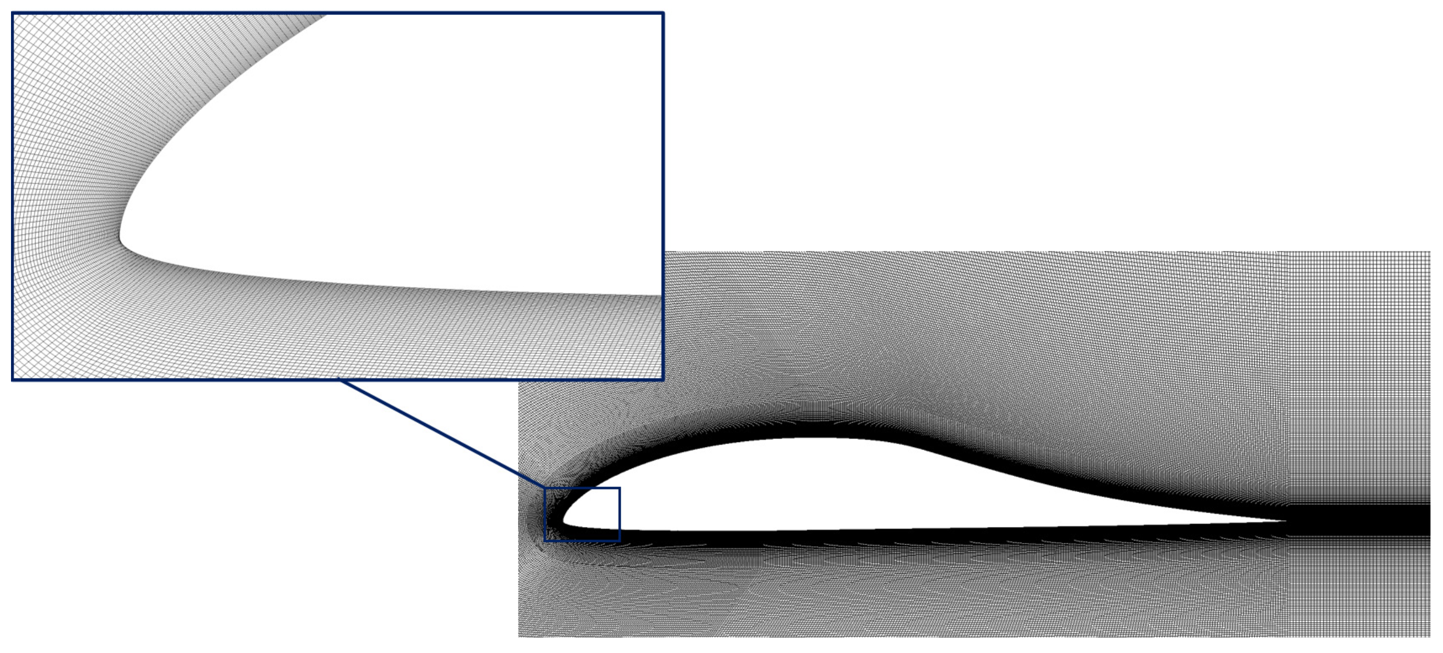
For numerical modeling of airfoil flow with turbulent viscosity, it is crucial to accurately resolve the near-wall viscous shear layers. This is essential to accurately calculate the integral aerodynamic characteristics in this application. To properly resolve the near-wall flow, some numerical models consider the use of near-wall functions that define the velocity profile by determining the velocity value as a function of the distance to the wall. Nevertheless, to compare various numerical models, including those that do not consider the use of near-wall functions, it is necessary to resolve the boundary layer by spatial discretization of the mesh for a relevant comparison of results. For this study, the necessary height of near-wall grid cells was determined by applying the $y^{+}=1$ criterion and a $\mathrm{Re}=1.5\times {10}^5$. Subsequently, the computational mesh was generated taking into account these wall cell dimensions.

The computational mesh has a block structure (C-mesh block structured computational mesh) and is two-dimensional, consisting of quasi-orthogonal quadrangular cells. Equidistant boundaries are constructed at a distance of 50 mm from the surface of the airfoil. Within these boundaries, the mesh gradually becomes denser toward the airfoil until it reaches the dimension of the element height, $h=2.5\times {10}^{-4}$ m ($y^{+}=1$). The view of the computational mesh is shown in Figure 3.

As the boundaries of the numerical domain are closed, where the atmospheric boundary conditions are set directly, the mesh becomes significantly coarser. The total number of cells is about 980 thousand.

The study examines the impact of steady flow on a suddenly stopped thick airfoil, which is initially entrained with the velocity of the flow. The study calculates the effects of angles of attack ranging from 0 to ${15}^{\circ }$. The convergence criterion is the achievement of the level of ${10}^{-4}$ by the value of the root-mean-square residual.

Calculations of unsteady flows result in chaotic oscillatory processes that are analyzed using statistical methods. For the airfoil, a quasi-periodic mode of change in aerodynamic characteristics is observed with periodic oscillatory changes occurring for integral parameters such as lift.

6. Numerical Method

To discretize the governing equations, the finite volume method on unstructured meshes is used [44]. Time integration is performed using the 3rd order Runge–Kutta method. The MUSCL scheme (Monotonic Upstream Schemes for Conservation Laws) is used to discretize inviscid fluxes, while viscous flows are obtained with the central scheme of 2nd-order accuracy. The MUSCL scheme enables the enhancement of the order of approximation in spatial variables while preserving the monotonicity of the solution, and it satisfies the TVD (Total Variation Diminishing) condition. It is a combination of 2nd order central finite differences and a dissipative term, which are switched between by a flow limiter built on the basis of characteristic variables.

The calculation of unsteady flow around a thick airfoil is completed when the self-oscillating regime is reached with a periodic change of local and integral characteristics in time. The time step corresponds to 0.01, and self-oscillation typically is reached in about 50 dimensionless units.

7. Characteristics of Model Airfoil

To examine differing turbulence models and choose an airfoil for further analysis, the flow encompassing the M06-13-128 airfoil is investigated, as shown in Figure 4 and for which experimental data are also available [23]. Varying the angle of attack between 0 and ${15}^{\circ }$, the assumed Reynolds number from experimentation is $\mathrm{Re}=1.5\times {10}^5$ with an airfoil chord of $L=1$ m. According to the given Reynolds number, the flowing velocity selected is $V=2.2$ m/s.

Figure 5 illustrates the flow pattern within the boundary layer at the laminar–turbulent transition zone. When the intermittency factor is 0, it denotes a laminar flow, while an intermittency factor of 1 indicates a turbulent flow. As the intermittency coefficient increases, the profiles of velocity in the boundary layer changes its character from laminar (smooth increase in velocity from zero) to turbulent (jump-like change in velocity), which causes a sharp increase in frictional drag. A comparison of calculations for fully turbulent flow and under free laminar–turbulent transition conditions indicates that the drag coefficient is most influenced by the boundary layer state.

The upper surface of the airfoil features a thin blue–green layer indicating laminar flow and a point of laminar–turbulent transition further ahead. The distance from the leading edge of this transition point varies depending on the angle of attack and falls around 0.55–0.6L.

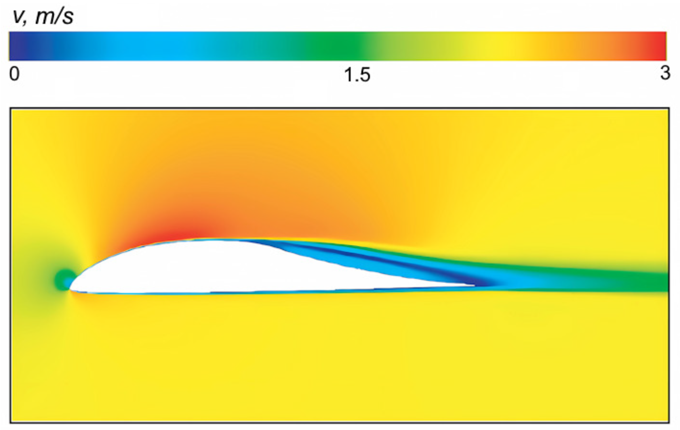
The velocity contours surrounding the airfoil are shown in Figure 6. Almost the entire lower surface of the airfoil, as well as the front upper surface, flow is laminar.

The numerical calculations of aerodynamic characteristics are presented in Figure 7, Figure 8 and Figure 9. Through the dimensionless lift force coefficient (Cl) and drag force coefficient (Cd), the aerodynamic parameters are expressed. Using a dimensionless form of forces allows a comparison of aerodynamic shapes, disregarding the size of the streamlined body and absolute velocity values. Dimensionless aerodynamic coefficients are defined by the equations

$$\begin{array}{cc}\hfill & C_l=\frac{2F_l}{\rho V^{2}S};\hfill \end{array}$$

(5)

$$\begin{array}{cc}\hfill & C_d=\frac{2F_d}{\rho V^{2}S}.\hfill \end{array}$$

(6)

where $F_l$ is the lift force, $F_d$ is the drag force, and S is the midsectional area.

The drag coefficient’s qualitative behavior when dependent on the angle of attack for thick and thin airfoils is similar: a larger angle of attack results in increased drag, particularly at large positive and negative angles.

Figure 10 shows the pressure distribution over the airfoil surface compared to the experiment [23] at zero angle of attack. The results show that the Transitional SST (tSST) model more accurately reproduces the pressure distribution over the airfoil surface, and it consequently allows for more accurate modeling of the airfoil separation zones.

The selection of a turbulence model has a significant impact on the calculation results. The airfoil coefficients vary in a fairly wide range of values. Neglecting the laminar–turbulent transition in turbulence models results in a significant underestimation of the drag coefficient. The exploitation of SST and Spalart–Allmaras (SA) models leads to coefficients that are two to three times lower than those obtained experimentally. The laminar model causes an overestimation of the drag coefficient by about 20–30%. However, the model considering the intermittency parameter shows a fairly good agreement with the experiment both in terms of numerical values and the way in which the values of the aerodynamic coefficient of the airfoil change with the variation of the angle of attack.

Separation of the boundary layer from the airfoil’s surface occurs even at a zero angle of attack, but detecting and evaluating this phenomenon’s influence on aerodynamic characteristics requires models that account for laminar–turbulent transition. The application of the SST model at an angle of attack of ${12}^{\circ }$ reveals a flow pattern with a significant separation zone. The use of the $\gamma$–${\mathrm{Re}}_{\theta }$ model for the external flow around the airfoil results in a larger separation zone that possesses a non-stationary nature. This phenomenon subsequently has an impact on the calculated characteristics.

8. Results and Discussion

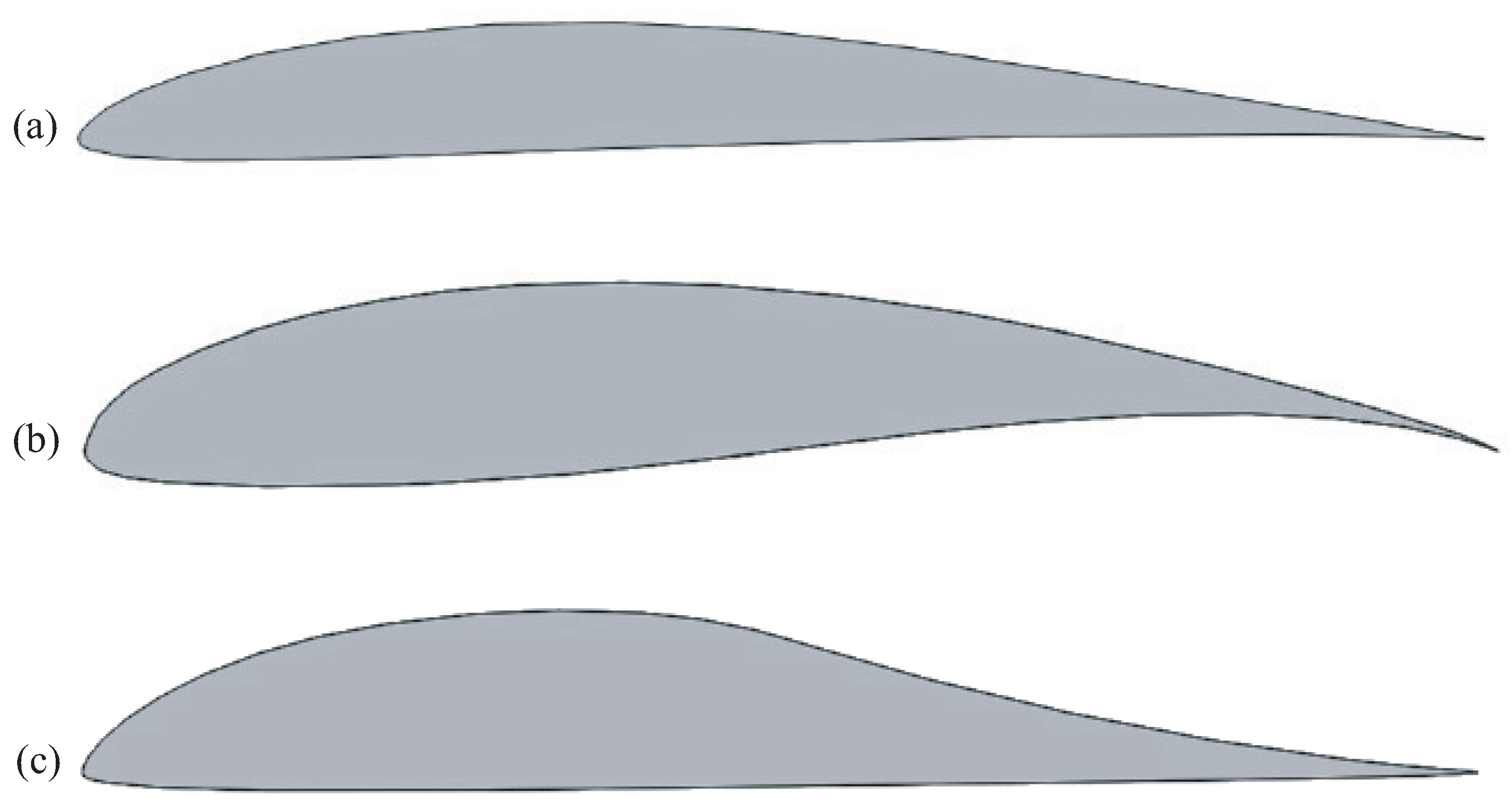
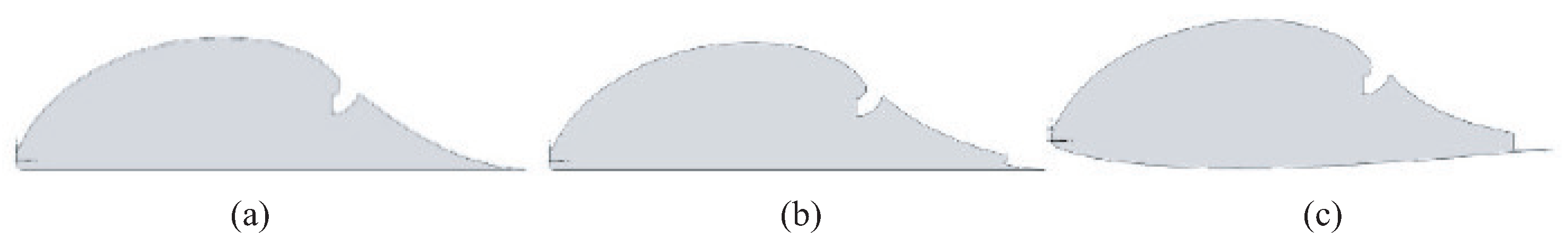
The calculations analyze multiple propulsion airfoils illustrated in Figure 11. A series of propulsion airfoils were generated by solving the inverse aerodynamics problem and utilizing stochastic global optimization methods [45]. Optimization methods based on solving the inverse problem of aerodynamics permit the consideration of the air sources and drains present on the wing’s surface in the aerodynamic profile. The concept of energetic methods of external streamline control necessitates the presence of air sources and drains for the operation of a propulsive wing. Therefore, the solution to this problem, including an air mass source and outflow, leads to the optimal shape of the propulsive airfoil. Airfoil 1 features a flat bottom surface, with no air flowing through the trailing edge (Figure 11a). Airfoil 2 also presents a flat lower surface, but air is blown through the trailing edge (Figure 11b). Airfoil 3 features an airfoil lower surface with increased thickness. Air is blown through the airfoil’s trailing edge, as shown in Figure 11c.

The airfoils have a large relative thickness and a favorable pressure gradient along most of the upper surface, which results in maintaining the laminar nature of the flow in this area and, consequently, a reduction in frictional drag. To provide rarefaction in the upper part of the airfoil, a suction slot located at the trailing edge is realized. Pressure at the tail section exceeds the front section. The pressure differential generates static thrust, which counteracts a substantial portion of the frictional resistance. In the event of air extraction being absent, these airfoils are inadequately streamlined bodies, whilst with adequate internal air flow, the tail section of the airfoil generates thrust.

Airfoil 1 corresponds to the airfoil analyzed by Ilyinsky [6], where experimental data are available for angles of attack ranging from 0 to ${10}^{\circ }$. As a result, modifications were made to the air sampling slot geometry and the section extending from the slot to the tail edge of the airfoil due to flow separation issues near the original sampling slot.

Aerodynamic profile 2 has a slotted nozzle on the trailing edge, which is complemented by an extended bottom plate to balance the pitching moment. This part also acts as a rudder, providing effective pitch control.

Airfoil 3 is a modified version of airfoil 2 that has a larger thickness. The lower surface profile allows for a significant improvement in lift due to the ground effect when at an angle of attack of $4^{\circ }$ and a distance from the surface of 10–30% of the airfoil chord. The nozzle area has increased by 50% compared to the original airfoil, allowing for a reduction in the speed of the jet flow to improve its propulsion. The trailing edge nozzle generates a reactive force at an angle of $-4^{\circ }$ when the aircraft is at zero angle of attack. This is designed to ensure that at the cruising angle of attack of $4^{\circ }$, the reactive force is parallel to the velocity vector.

The free flow velocity is assumed to be 70 m/s, which corresponds to the Reynolds number $\mathrm{Re}=1.5\times {10}^5$. In the air exhaust slot, the degree of flow rarefaction is set to $r=p_s-p$, where $p_s$ is the pressure at the edge of the slot and p is the local pressure. In the calculations, the degree of flow rarefaction varies from 0 to $-0.5$ atm. For each pressure value in the slot and for each angle of attack, the dimensionless airflow $q=Q/\left(Vbl\right)$ is calculated from the airfoil surface, where Q is the volumetric airflow, V is the velocity of the external flow, L is the chord of the airfoil, and l is the length of the airfoil section, which is equal to 1 m.

The flow rate of the exhaust air for a given degree of rarefaction remains constant until boundary layer separation occurs, after which the flow rate decreases (Figure 12). This is caused by the formation of a circulating flow zone at the trailing edge of the airfoil, where the pressure is lower than in the case of continuous flow. The decrease in pressure drop is accompanied by a decrease in bleed air flow.

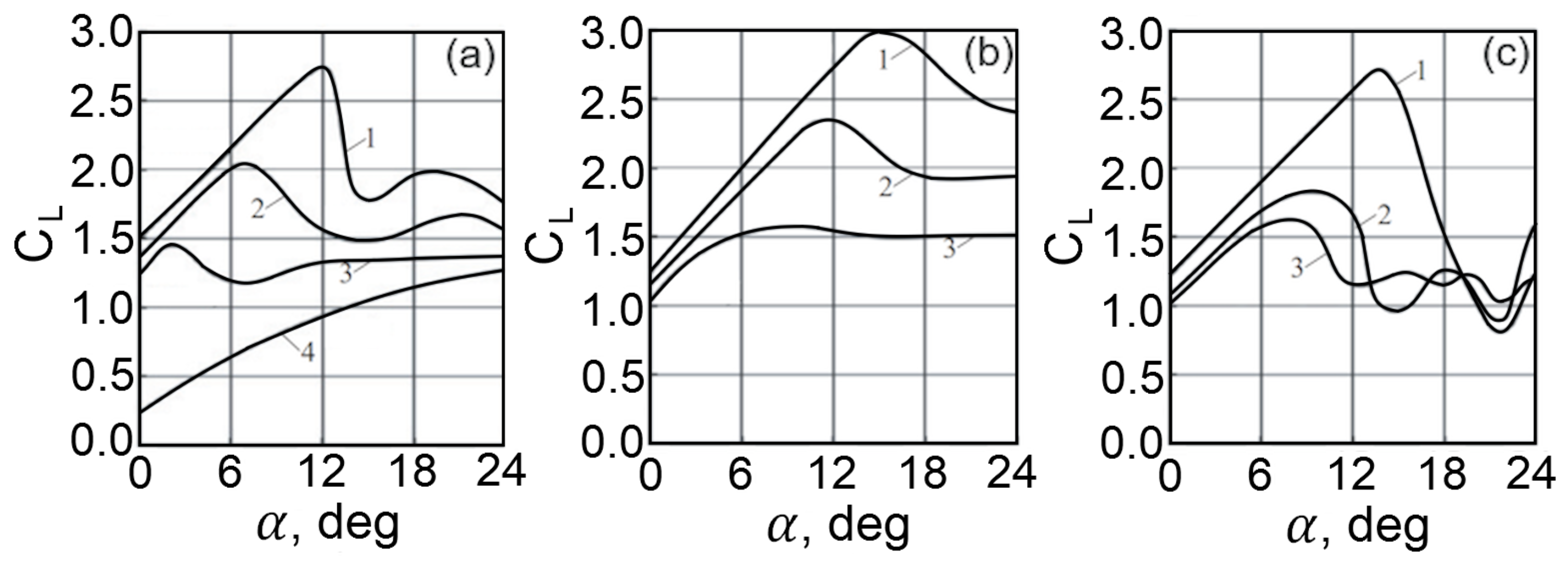
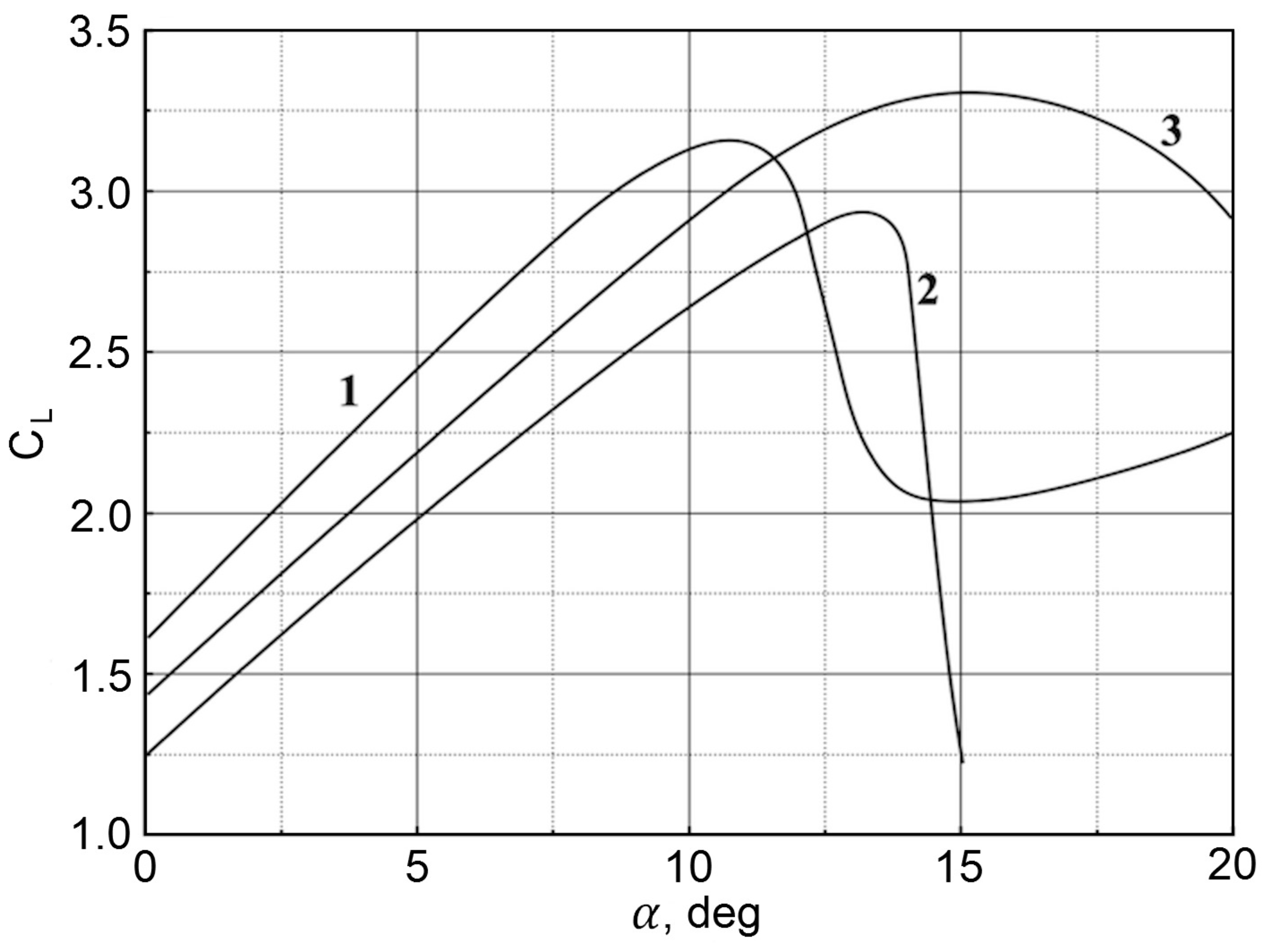
A comparison of the lift coefficients is given in Figure 13 as a function of the angle of attack of the airfoil and the degree of rarefaction in the slot. The airfoils are relatively thick and have a favorable pressure gradient along most of the upper surface, which results in maintaining the laminar nature of the flow in this area and reducing frictional drag. The suction slot is located upstream of the trailing edge and is used to create a burst pressure increase at the top of the airfoil. As a result, the pressure on the trailing edge is greater than the pressure on the leading edge. This difference creates a static thrust that compensates for a significant portion of the frictional drag.

As the degree of rarefaction increases, the lift coefficient of airfoil 1 increases, and the limiting angle of attack of the continuous flow increases (Figure 13a). In this case, the dependencies corresponding to the degrees of rarefaction $r=-0.4$ atm and $r=-0.5$ atm practically coincide; therefore, it is assumed that at $r=-0.5$ atm, the limiting characteristics of airfoil 1 are reached.

For airfoil 2, the amount of ejected air is assumed to be equal to the amount taken in through the slot. The ejection of the jet delays the onset of stalled flow regimes. At the same time, the maximum lift coefficient is almost 10% higher than the value corresponding to airfoil 1 (Figure 13b).

For airfoil 3, it is also assumed that the amount of air ejected through the nozzle is equal to the amount received through the slot. At the same time, the improved airfoil 3 is slightly inferior to airfoil 2 in terms of maximum lift coefficient. Airfoil 3 has a nozzle set at an angle of $-4^{\circ }$, which reduces the lift force of the airfoil. Calculations show that at $r=-0.5$, increasing the airflow through the trailing edge nozzle from 50 to 200% of the airflow through the slot leads to a monotonic increase in lift, starting at the angle of attack $4^{\circ }$ (angle of attack at which the vertical component of the thrust vector becomes zero). At lower degrees of rarefaction, the effect of the flow rate of air ejected through the trailing edge nozzle on the lift force is less pronounced.

There is an optimum flow rate of air extracted from the surface at which the viscous friction drag is minimal. This is explained by the fact that the laminar section of the flow reaches its maximum length at the optimum air extraction rate. When the extraction rate is further increased, the resistance in the laminar boundary layer increases because the velocity of external flow increases.

The change in air flow is achieved by controlling the degree of rarefaction in the slot $\Delta p$. For each angle of attack, $\Delta p$ increases as long as the lift coefficient increases. Practical convergence is achieved at $\Delta p=-0.5$ atm.

Up to an angle of attack of 12 degrees, the lift coefficient increases almost linearly (Figure 14), reaching a value of 3–3.3. The lift force increases as the degree of rarefaction in the air sampling slot increases, reaching the limit value at a rarefaction of 0.5 atm. At maximum vacuum, the lift force is increased as more air is ejected through the trailing edge with the strength of this effect increasing as the flow rate grows. At low rarefaction, the situation is uncertain. Specifically, the exhaust jet may also decrease lift. The slot’s optimal location is near the airfoil’s trailing edge. Additional movement of the slot toward the trailing edge results in the establishment of an unsteady separated flow regime and a decrease in its aerodynamic characteristics.

9. Conclusions

To achieve the optimal airfoil, taking into account gas extraction from its surface and blowing through the trailing edge, a method is used to solve the inverse problem of aerodynamics (design of the airfoil shape according to given flow parameters near the airfoil). The calculations performed demonstrate the significant impact of laminar–turbulent transition on the aerodynamic characteristics of the airfoil when Reynolds numbers are low. The calculations utilized the $\gamma$–${\mathrm{Re}}_{\theta t}$ turbulence model, which considers the shift from laminar to turbulent flow regimes.

The aerodynamic features of airfoils that implement air extraction at the upper critical point to increase lift have been studied. Traction is created by the section of the upper surface of the airfoils from the air intake slot to the trailing edge even when there is no air outlet slot in the trailing edge. The lift force rises as the degree of rarefaction formed in the air sampling slot increases, approaching the limit value at a specific degree of rarefaction. At maximum vacuum pressure, the ejection of air through the trailing edge results in an increased lift force, which becomes larger as the flow rate increases. The situation becomes ambiguous at low rarefaction, as in this case, the exhaust jet may also decrease the lift.

The analyzed airfoils possess substantial relative thickness (up to 38%) and carrying capacity, generating thrust without blowing through the trailing edge. These characteristics make them suitable for integration into the aircraft’s airframe design particularly when the internal compartment volume is a crucial factor.