Article

Parallel Bootstrap-Based On-Policy Deep Reinforcement Learning for Continuous Fluid Flow Control Applications

MINES Paristech, CEMEF, PSL—Research University, 06904 Sophia Antipolis, France
*
Author to whom correspondence should be addressed.
Fluids 2023, 8(7), 208; https://doi.org/10.3390/fluids8070208
Submission received: 17 May 2023 / Revised: 5 July 2023 / Accepted: 11 July 2023 / Published: 14 July 2023
(This article belongs to the Section Mathematical and Computational Fluid Mechanics)

Abstract

:
The coupling of deep reinforcement learning to numerical flow control problems has recently received considerable attention, leading to groundbreaking results and opening new perspectives for the domain. Due to the usually high computational cost of fluid dynamics solvers, the use of parallel environments during the learning process represents an essential ingredient to attain efficient control in a reasonable time. Yet, most of the deep reinforcement learning literature for flow control relies on on-policy algorithms, for which the massively parallel transition collection may break theoretical assumptions and lead to suboptimal control models. To overcome this issue, we propose a parallelism pattern relying on partial-trajectory buffers terminated by a return bootstrapping step, allowing a flexible use of parallel environments while preserving the on-policiness of the updates. This approach is illustrated on a CPU-intensive continuous flow control problem from the literature.

1. Introduction

Deep neural networks (DNNs) have become a pervasive approach in a large variety of scientific domains in the course of the last decade, achieving multiple breakthroughs in domains such as image classification tasks [1,2], speech recognition [3] or generative tasks [4,5]. Thanks to cheaper hardware and generalized access to large computational resources, such advances have led to a general evolution of the reference methods at both academic and industrial levels.
Among these developments, decision-making techniques have largely benefited form the coupling of DNNs with reinforcement learning algorithms (called deep reinforcement learning, or DRL), due to their feature extraction capabilities and their ability to handle high-dimensional state spaces. Unprecedented efficiency has been achieved in many domains such as robotics [6], language processing [7], or games [8,9], but also in the context of industrial applications [10,11,12].
In recent years, DRL-based approaches have made their way into the domain of flow control, with an increasing amount of contributions on varied topics such as (but not limited to) drag reduction [13], collective swimming [14] or heat transfers [15]. Although a handful of couplings of DRL with experimental setups were reported, most contributions make use of numerical environments relying on computational fluid dynamics (CFD) solvers [16,17], making the performance of the latter an important lever for the successful learning of a control strategy by a DRL agent. Yet, in order to control processes of increasing computational loads, the use of parallel environments to accelerate the sample collection between agent updates also appears as a key ingredient, allowing to further exploit existing resources and reducing the time-to-control (here defined as the computational time required to reach efficient control). In 2019, such setup was introduced by Rabault and Kuhnle in the context of flow control for the drag reduction on a cylinder at low Reynolds number [18]. In this contribution, the authors showed that, for a configuration where the CFD time represents almost 100% of the time-to-control, using a parallel collection of samples could yield an excellent speedup up to the point where the number of parallel environments (hereafter denoted as  n env ) becomes equal to the number of full episodes used for a single update (hereafter denoted as  n update , in this case equal to 20 episodes). Pushing the parallelization process beyond this point resulted in “over-parallelization” (sic) and led to observable flat steps in the learning process (see [18], Figure 4).
Although efficient, the approach introduced above comprises two major drawbacks. First, the “over-parallelization process” inherently leads to off-policy updates of the agent (i.e., the agent is trained with samples produced by a previous policy), which introduces bias in the policy gradient estimates and increases the risk of the agent falling into local optima. While importance sampling corrections could be used to account for the discrepancy between the current policy and the behavior policy, such an approach is known to introduce large variance in the estimate and require additional tuning [19,20]. Second, in order to take maximum advantage of the parallel sample collection, this approach constrains the size of the buffer update to be (i) a multiple of the number of transitions within an episode, and (ii) a multiple of the number of parallel environments. These two points may lead either to a suboptimal control model or to a suboptimal use of the available computational resources. To overcome these issues, we propose an update approach based on partial trajectories terminated by a return bootstrapping step to mimic a continuing environment (i.e., the last reward of each parallel update buffer is modified to account for the continuous nature of the control task). The concept of partial trajectories is not new and was, for example, presented by Schulman in the original proximal policy optimization (PPO) paper (see [21], Section 5), while the bootstrapping method was originally proposed by Pardo et al. [22]. As will be shown below, the combination of these two approaches allows us to design a flexible parallel sample collection pattern, while retaining the on-policiness of the PPO algorithm (i.e., the agent is trained with samples produced by the current policy). This represents a major asset in the context of fluid flow control, where efficient parallel sample collection eventually allows the control of complex, CPU-intensive environments.
The present paper is organized as follows: in Section 2.1, a short reminder of the basics of on-policy DRL algorithms and proximal policy optimization is provided. Then, a recall is made on the bootstrapping technique in Section 2.3, after which the proposed bootstrapped partial trajectories approach is detailed in Section 2.4. To benchmark the proposed method, a continuous flow control case from the literature is presented in Section 3 (namely the control of a falling fluid film, adapted from [23]). This case is then exploited in Section 4 to benchmark (i) the interest of bootstrapping and (ii) the proposed parallel paradigm. Finally, conclusions and perspectives are given.

2. Parallel Bootstrap-Based on-Policy Deep Reinforcement Learning

2.1. On-Policy DRL Algorithms

Policy-based methods maximize the expected discounted cumulative reward of a policy  π ( a | s )  mapping states to actions, resorting to a probability distribution over actions given states. Among these techniques, two types of algorithms must be differentiated:
Fluids 08 00208 i001
on-policy algorithms usually require that the samples they use for training are generated with the current policy. In other words, after having collected a batch of transitions using the current policy, these data are used to update the agent and cannot be re-used for future updates;
Fluids 08 00208 i001
off-policy algorithms are able to train on samples that were not collected with their current policy. They usually use a replay buffer to store transitions, and randomly sample mini-batches from it to perform updates. Hence, samples collected with a given policy can be re-used multiple times during the training procedure.
Although off-policy algorithms naturally exhibit a better sample efficiency, their stability is not guaranteed, and, as of today, they have not yet made their way in the DRL-based flow control domain [17]. Contrarily, although less sample-efficient, on-policy algorithms present good stability properties, ease of implementation and tuning, and are widely represented in the field of DRL-based flow control. By focusing on on-policy algorithms, the present study can deliver more useful insights to the community. In the following section, we focus on the details of the well-known PPO algorithm [21].

2.2. Proximal Policy Optimization (PPO)

The PPO algorithm belongs to the class of actor-critic methods [24], in which an actor provides actions based on observations by sampling from a parameterized policy  π θ , while a critic is devoted to evaluate the future expected discounted cumulative reward. The standard loss used to update the actor network reads:
L ( θ ) = E τ π θ t = 0 T log π θ ( a t | s t ) A π θ ( s t , a t ) ,
where  A π θ ( s , a )  is the advantage function, that represents the improvement in the expected cumulative reward when taking action a in state s, compared to the average of all possible actions taken in state s. The advantage function is evaluated thanks to the rewards collected from the environment, and the evaluation of the value function is provided by the critic. Although displaying good performance, vanilla actor-critic techniques displayed a high sensitivity to the learning rate, with small learning rates implying slow learning, while large learning rates leading to possible performance collapses. To overcome these issues, the proximal policy optimization [21] uses a simple yet effective heuristic that helps avoid destructive updates. Namely, it relies on a clipped surrogate loss:
L ( θ ) = E ( s , a ) π θ old min π θ ( a | s ) π θ o l d ( a | s ) , g ϵ , A π θ old ( s , a ) A π θ old ( s , a ) ,
where
g ( ϵ , A ) = ( 1 + ϵ ) A if A 0 , ( 1 ϵ ) A if A < 0 ,
and  ϵ  is the clipping range, a small user-defined parameter defining how far away the new policy is allowed to go from the old one. Due to its improved learning stability and its relatively robust behaviour with respect to hyper-parameters, the PPO algorithm has received considerable attention in the DRL community, including in the context of flow control [17].
It seems worth noting that, in practice, although PPO is considered an on-policy method in the sense that it does not make use of a replay buffer, it is not strictly on-policy, as the collected transitions will be used for multiple epochs in the course of a single update before being discarded. This fact leads a part of the community to label PPO as an off-policy method, which is fundamentally correct, although in essence the method is fundamentally different from state-of-the-art off-policy methods such as deep deterministic policy gradients-like methods (DDPG [25], TD3 [26]).

2.3. Bootstrapping

DRL methods can be used either to tackle episodic or continuous tasks. In episodic tasks, the agent has a limited amount of time to successfully reach a given goal, the provided time limit being an intrinsic characteristic of the problem (for example, the case of a robotic arm moving an object from an initial position to a final position). In continuous tasks, the time limit is often arbitrary, the control being supposed to run indefinitely (for example, the case of active drag reduction around an obstacle). In the case of continuous control, the time limit is set only so the environment can be regularly reset during the training, leading to an improved diversity of samples and a good representation of all the stages of control. In the context of on-policy algorithms such as PPO, this distinction leads to a subtle yet capital difference in the way the advantage buffer must be terminated when an episode is ended for a time-out reason [22]. Traditionally, once an episode is terminated, the advantage vector is assembled using the reward vector  r  collected from the environment during the episode, the estimated value vector  v ^ π θ  that estimates the discounted cumulative reward starting from a given state until the end of the episode, and the termination mask  m , whose values are equal to 1 for each non-terminal state, and 0 for terminal states (so on a single episode, the termination mask is typically a vector of 1 terminated with a 0). Then, the advantage vector can be assembled as shown in Algorithm 1.
Algorithm 1 Traditional advantage vector assembly
1:given: the reward vector  r
2:given: the value vector  v ^ π θ
3:given: the termination mask  m
4:for   t = 0 , n steps 1 do
5:        y t = r t  if  s t  is terminal else y t = r t + γ v ^ π θ ( s t + 1 )
6:end for
7:for   t = n steps 2 , 0  do
8:        y t = y t + γ m t y t + 1
9:end for
10:  A = y v ^ π θ
The computed advantage vector is later used in the computation of the actor loss (here, the computation of the standard advantage function is presented for simplicity, yet the comments made in this section still hold for more complex advantage functions, such as the generalized advantage estimate [27], for example). Yet, the Algorithm 1 does not account for terminations due to time limits in the context of continuous tasks. Hence, when trained, providing such an advantage vector to the agent does not account for the possible future rewards that could have been experienced if a different arbitrary time limit had been used. Moreover, this approach inherently brings a credit attribution problem: reaching a similar state in the course of an episode or on a time-out termination would lead to very different outcomes that would be evaluated with the same inaccurate value function estimate  v ^ π θ ( s t ) , thus leading to a degraded learning process. However, a fairly simple remedy called bootstrapping consists in replacing the “if  s t  is terminal” condition of Algorithm 1 by “if  s t  is terminal and not a time-out”. Indeed, one can clearly see from Algorithm 1 at line 8 that modifying the final target value  y t  in the case of a time-out (i.e.,  t = T ) will modify all the previous target values  y t < T , thus having a large impact on the actor update, and eventually leading to a significant performance improvement. Experiments using bootstrapping alone in the context of continuous flow control tasks are presented in Section 4.1. Additional results on regular benchmark control tasks from the gym and mujoco packages are also provided in Appendix A.

2.4. Parallel Bootstrap-Based Learning

In the context of CPU-expensive CFD environments, speeding up the training of DRL agents by harnessing the capabilities of parallelism can lead to substantial gains in computational resources. Although this can be accomplished by exploiting the inner parallelism of the CFD computation itself, collecting data from environments running in parallel is also a well-known technique that has largely spread in the community. In the context of the coupling of CFD environments with DRL, such improvement represents a key ingredient for the discovery of efficient control laws, as the environment can represent from 80% to more than 99% of the computational time. In [18], the authors consider a 2D drag reduction case using the PPO algorithm, setting the update frequency of their agent to  n update = 20  episodes. Using an asynchronous parallelism of the environments, the authors report an excellent speedup up to  n env = 20  parallel environments, and a decent performance improvement up to 60. Yet, for  n env > n update , a fraction of the updates are naturally performed in an off-policy way, due to the fact that the samples used were produced using a different policy than the one being updated. Although an appreciable speedup is still observed, this choice can lead to a degraded learning, as will be evidenced in Section 4.2. Here, we propose to exploit the bootstrapping technique presented above to design a synchronous parallel paradigm that respects the on-policy nature of PPO.
The proposed method is illustrated in Figure 1 for a simple configuration: a regular episode consists of four transitions, and for this example it is decided that an update of the agent requires  n update = 2  full episodes, or eight transitions. For  n env = 1 , two episodes are unrolled sequentially between each update. For  n env = 2 , transition sampling is effectively sped up while retaining the same update pattern, as two full episodes can be collected between each agent learning step. However, when reaching  n env = 4 , four full episodes are collected at once, and are then used to form two update buffers. While the first update will be on-policy, the second one will violate the on-policiness of the method, leading to possibly sub-optimal control. The proposed partial-trajectory approach holds two major differences: first, all collected transition buffers are terminated with a return bootstrap step; second, in the case of  n env = 4 , only two transitions are unrolled for each environment, and a first buffer update is formed using four partial bootstrapped trajectories. Once the update is performed, the second half of the episodes is unrolled using the updated policy, forming a second update buffer used for a second on-policy update. For convenience, in the remainder of this paper, we call the first kind end-of-episode (EOE) bootstrapping, while the second kind is designated as partial-trajectory (PT) bootstrapping. Regarding the implementation of these features, adding EOE bootstrapping to an existing actor-critic code requires only minimal modifications, while PT bootstrapping requires a larger amount of modifications in the unrolling process.
In the context of real environments, this approach leads to an important flexibility, as (i) it does not need to collect full episodes to perform updates, (ii) it allows for better exploitation of parallel environments, and (iii) it preserves the on-policiness of the PPO algorithm. While it is important to notice that this method relies on a proper evaluation of the value function at the states at which bootstrapping is applied, our experiments show that the learning of the value function in the early steps of the process is sufficient for the method to bring an important benefit over the vanilla approach.

3. Continuous Flow Control Application

To illustrate the interest of the approach introduced in the previous section, a continuous flow control case from the literature is considered. To present meaningful results, the authors chose an environment for which the CPU cost of the unrolling is significantly higher than the training of the agent (typically around  96 %  of the total CPU time). To illustrate, the repartition of the CPU time of these two cases is compared with that of the well-known pendulum-v1 environment in Figure 2. This section is devoted to the description of the cases, while the corresponding results are shown in Section 4.

3.1. Control of Instabilities in a Falling Fluid Film

The considered case concerns the control of growing instabilities developing in a 1D falling fluid film perturbed with random noise, for which a simplified, two-equations model for this setup was proposed in 1967 by Shkadov [28]. Although it was found to lack some physical consistency [29], this model displays interesting spatio-temporal dynamics while remaining acceptably cheap to integrate numerically. It simultaneously evolves the flow rate q as well as the fluid height h as:
t h = x q , t q = 6 5 x q 2 h + 1 5 δ h 1 + x x x h q h 2 ,
with all the physics of the problem being condensed in the  δ  parameter:
δ = 1 15 3 R e 2 W 1 3 ,
where  R e  and W are the Reynolds and the Weber numbers, respectively, defined on the flat-film thickness and the flat-film average velocity [30]. The system (1) is solved on a 1D domain of length L, with the following initial and boundary conditions:
q ( x , 0 ) = 1 and h ( x , 0 ) = 1 , q ( 0 , t ) = 1 and h ( 0 , t ) = 1 + U ( ε , ε ) , x q ( L , t ) = 0 and x h ( L , t ) = 0 ,
with  ε 1  being the noise level. As shown in Figure 3, the introduction of a random uniform noise at the inlet triggers the development of exponentially growing instabilities (blue region) which eventually transition to a pseudo-periodic behavior (orange region). Then, the periodicity of the waves break, and the instabilities turn into into pulse-like structures, presenting a steep front preceded by small ripples [31]. It is observed that some of these steep pulses, called solitary pulses, travel faster than others, and can capture upstream pulses in coalescence events. The dynamics of these solitary pulses are fully determined by the  δ  parameter, while the location of the transition regions also depends on the inlet noise level [30].
The control environment proposed here is re-implemented based on the original publication of Belus et al. [23], although with some significant differences, noted hereafter. It is important to notice that the translational invariance feature introduced in [23] is not exploited here. Equations (1) are discretized using a finite difference approach. Due to the existence of sharp gradients, the convective terms are discretized using a TVD scheme with a minmod flux limiter. The discretized third-order derivative is obtained by chaining a second-order centered difference for the second derivative, chained with a second-order forward difference, leading a second-order approximation. Finally, the time derivatives are discretized using a second-order Adams-Bashforth method. The convergence of the numerical discretization is tested on a manufactured solution in Appendix B.
The control of the system (1) is performed by adding a forcing term  δ q j  to the equation driving the temporal evolution of the flow rate. In practice, this is achieved by adding localized jets at certain positions in the domain, as shown in Figure 4, whose strengths are to be controlled by the DRL agent. The first jet is positioned by default at  x 0 = 150 , with jet spacing being by default set to  Δ x jets = 10 , similarly to [23]. To save computational time, the length of the domain is a function of the number of jets  n jets  and their spacing:
L = L 0 + n jets + 2 Δ x jets .
By default,  L 0 = 150  (which corresponds to the start of the pseudo-periodic region for  δ = 0.1 ), and  n jets  is set equal to 1. The spatial discretization step is set as  Δ x = 0.5 , while the numerical time step is  Δ t = 0.005 . The inlet noise level is set as  ε = 5 × 10 4 , similarly to [23]. The injected flow rate  δ q j  has the following form:
δ q j ( x , t ) = A u j ( t ) 4 x x j l x j r x x j r x j l 2 ,
with  A = 5  an ad-hoc non-dimensional amplitude factor,  x j l  and  x j r  the left and right limits of jet j, and  u j ( t ) [ 1 , 1 ]  the action provided by the agent. Expression (5) corresponds to a parabolic profile of the jet in x, such that the injected flow rate drops to 0 on the boundaries of each jet. The jet width  x j r x j l  is set equal to 4, similarly to [23]. The time dependance of  u ( t )  is implemented as a saturated linear variation from an action to the next one, in the form
u j ( t ) = ( 1 α ( t ) ) u j n 1 + α ( t ) u j n , with α ( t ) = min t t n Δ t int , 1 ,
Hence, when the actor provides a new action to the environment at time  t = t n , the real imposed action is a linear interpolation between the previous action  u j n 1  and the new action  u j n  over a time  Δ t int  (here taken equal to  0.01  time units); after that, the new action is imposed over the remaining action time  Δ t const  (here taken equal to  0.04  time units). The total action time-step is therefore  Δ t act = Δ t int + Δ t const , whose value is therefore equal to  0.05  time units. The total episode time is fixed to 20 time units, corresponding to 400 actions.
The observations provided to the agent are the mass flow rates collected in the union of regions  A obs j  of length  l obs = 10  located upstream of each jet, as shown in Figure 4. Contrarily to the original article, the flow rates of this region are not provided to the agent, and the observations are not clipped. The reward for each jet j is computed on a region  A rwd j  of length  l rwd = 10  located downstream of it (see Figure 4), the global reward consisting of a weighted sum of each individual reward:
r ( t ) = 1 l rwd n jets j = 0 n jets 1 x A rwd j ( h ( x , t ) 1 ) 2
Finally, each episode starts by randomly loading a fully developed initial state from a pre-computed set. The latter were obtained by solving the uncontrolled equations from an initial flat film configuration during a time  t init  and comprise between 200 and 220 time units.

3.2. Default PPO Parameters

The default parameters used for the present study are presented in Table 1. A PPO agent is used with separate networks for the actor and the critic, the actions being drawn from a multivariate normal law with diagonal covariance matrix. While the critic network is a simple feedforward network with two hidden layers of size 64, the actor network is made of a trunk of size 64, with two branches composed of a single layer, each of size 64. The first branch is terminated using a tanh layer, used to output the mean of the normal distribution, while the second branch ends with a sigmoid layer, used to output the standard deviation of the distribution. The actions drawn from the corresponding distribution are clipped in  [ 1 , 1 ] d  before being mapped to their adequate physical range. The generalized advantage estimate [27] is used, and the advantage vectors are normalized per rollout. Additionally, we underline that the current parallel implementation is based on the message-passing interface (MPI), which led to improved parallel speedups over shared-memory approach.

4. Results

In this section, we evaluate the interest of bootstrapping, as well as the performance of the proposed parallel paradigm against the canonical parallel approach. First, we simply compare the score curves obtained from sequential learning, with and without the end-of-episode (EOE) bootstrapping step. Then, we investigate the performance of the partial-trajectory (PT) bootstrapping parallel technique against the standard approach. Since they do not represent the core of this contribution, results from the solved environment are proposed in Appendix C.

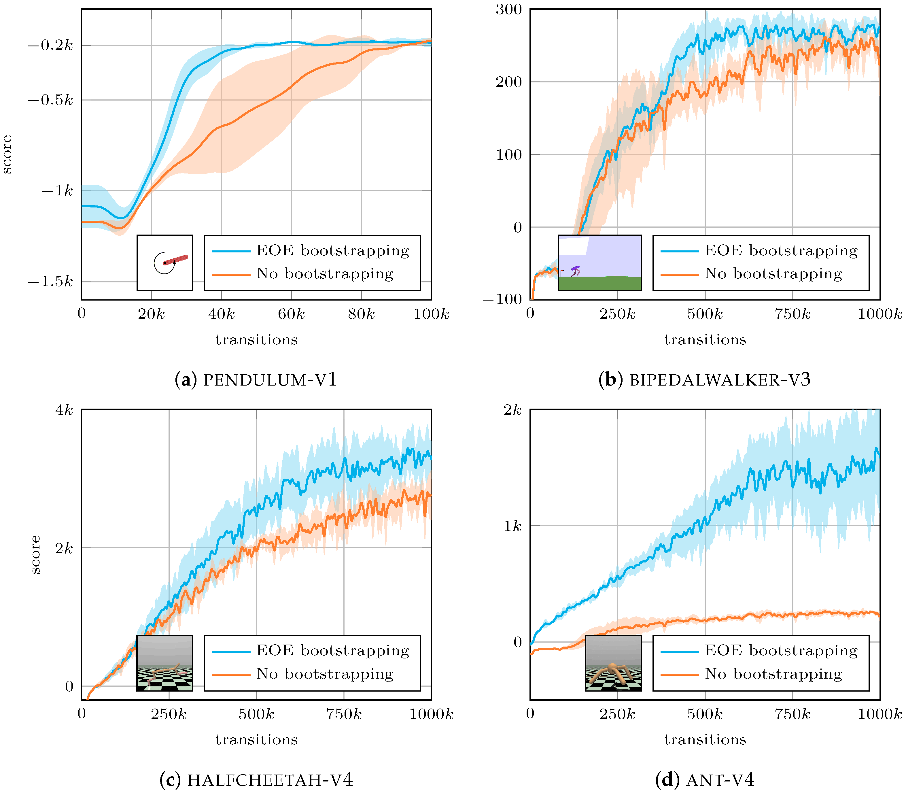
4.1. End-of-Episode Bootstrapping

First, we consider the sole impact of EOE bootstrapping on the agent training. To do so, we compare the score curves obtained by training an agent in sequential mode on both environments, with a “regular” ending (i.e., no EOE bootstrapping step) and with a bootstrapped ending. As can be observed in Figure 5, EOE bootstrapping accelerates the convergence of the agent while also reducing the variability in performance between the different runs. On the Shakdov environment, it almost cuts by half the number of required transitions to reach the maximal score. To illustrate further the benefits of EOE bootstrapping, results on standard gym environments are also presented in Appendix A. Similar conclusions are drawn from these additional examples.
To better understand the effects of the EOE bootstrapping, the plots of the value loss and value estimate along the course of training are proposed in Figure 6a,b, respectively. A significantly lower value loss is observed, indicating that the EOE bootstrapping, by solving the credit assignment issue [22], induces a smoother value landscape for the critic to learn. This results in higher value estimates, which is expected due to the nature of the EOE bootstrapping procedure.

4.2. Bootstrap-Based Parallelism
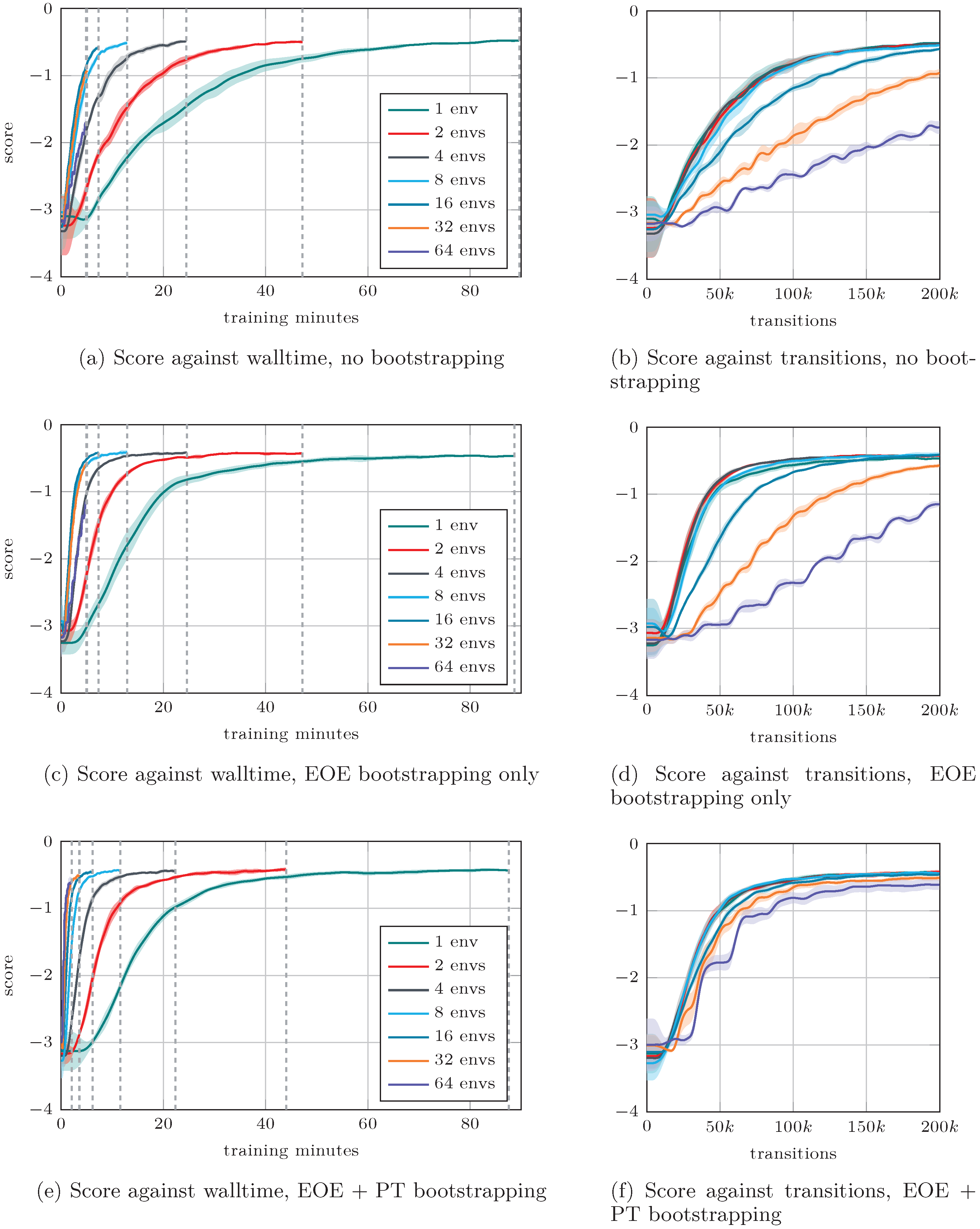
This section focuses on the interest of the partial-trajectory (PT) bootstrapping technique for parallel transitions collection proposed in Section 2.4. To evaluate its interest, we consider the score curves obtained on the Shkadov environment in different configurations, the number of parallel environments ranging from 1 to 64 (see Figure 7). First, we solve it with no bootstrapping at all (Figure 7a,b), then with EOE bootstrapping only (Figure 7c,b), then with EOE and PT bootstrapping (Figure 7e,f). In all three cases, the score curves are plotted both against walltime and transitions in order to visualize the parallel speedup obtained, as well as the relative performances using different numbers of parallel environments. For the clarity of the following discussion, we remind the reader that  n env  designates the number of parallel environments used to gather transitions, and  n update  the number of full episodes to perform an update of the agent (here equal to 8). Moreover, we introduce the notation  s n m M  to designate the speedup observed for a parallel approach M when using m parallel environments instead of n. Hence, for a perfect speedup,  s n m M = m n .
Fluids 08 00208 i001
For  n env n update ,the performance remains stable in each of the three configurations. This is expected, as the use of parallel environments only modifies the pace at which the updates occur, but the constitution of the update buffers is the same as it would have been for  n env = 1 . Yet, the use of EOE bootstrapping leads to a faster convergence than the regular case, as was already observed in previous section. Moreover, as PT bootstrapping does not occur when full episodes are used, Figure 7d,f present similar results for  n env 8 ;
Fluids 08 00208 i001
For  n env > n update , a rapid decrease in convergence speed and final score is observed for the regular approach, with  n env > 16 , resulting in very poor performance (Figure 7b). This illustrates the reasons that motivated the present contribution, i.e., that the standard parallel paradigm results in impractical constraints, which prevents massive environment parallelism. Introducing EOE bootstrapping (Figure 7d) improves the situation by (i) generally speeding up the convergence, and (ii) improving the final performance of the agents, although the final score obtained for  n env = 32  remains sub-optimal, while that of  n env = 64  is poor. Additionally, the “flat steps” phenomenon described in [18] clearly appears for  n env = 32  and 64, with the length of the steps being roughly equal to the number of transitions unrolled between two updates of the agent. When adding PT bootstrapping (Figure 7f), a clear improvement in the convergence speed is observed even for large  n env  values, and the gap in final performance significantly reduces. The flat steps phenomenon is still observed in the early stages of learning for  n env = 32  and 64, although with significantly reduced intensity.
Fluids 08 00208 i001
Similarly to [18], we observe decent speedups for  n env n update , with  s 1 8 EOE + PT = 7.6 , against  s 1 8 regular = 6.9 . This difference is attributed to the additional buffering overhead required in the regular approach, as more transitions are unrolled and stored between each update compared to PT bootstrapping. For higher numbers of parallel environments, we measure  s 1 32 EOE + PT = 25.4  against  s 1 32 regular = 17.7 , and  s 1 64 EOE + PT = 42.4  against  s 1 64 regular = 18.4 . Again, the excessive memory and buffering requirements of the regular case are the most probable cause of this discrepancy, as is evidenced by the fact that  s 1 64 regular s 1 32 regular . In the present case, we underline that speedups could probably be improved by replacing the computation of a random initial state at each reset step of the environment by the loading of pre-computed initial states from files.
Hence, the introduction of EOE and PT bootstrapping roughly enables the use of four times more parallel environments than with the vanilla parallelism, thus reducing the resolution time of the Shkadov environment from nearly 1.5 h to approximately 2 min while retaining the same final performance.

5. Conclusions

In the present contribution, we introduced a bootstrapped partial trajectory approach for parallel environments, in order to speed up learning for deep reinforcement learning agents while retaining their on-policiness. The proposed method was tested on a CPU-intensive flow control case from the literature, bringing multiple improvements over regular approaches such as (i) faster convergence, (ii) improved performance for  n env > n update , (iii) improved parallel speedups, (iv) increased flexibility regarding the compatibility of  n env  and  n update , and (v) preserved on-policiness. The new parallel paradigm roughly allowed for the safe exploitation of four times more parallel environments than the vanilla approach, and speedups as high as 42 were measured. Such techniques, coupled with an efficient parallelism at the solver level, open the door to the control of more complex, resource-demanding environments, thus pushing forward the current limits of DRL-based fluid flow control.

Author Contributions

Conceptualization, J.V.; Methodology, J.V.; Software, J.V.; Validation, J.V.; Writing—original draft, J.V.; Writing—review & editing, E.H. All authors have read and agreed to the published version of the manuscript.

Funding

Funded/co-funded by the European Union (ERC, CURE, 101045042). Views and opinions expressed are however those of the author(s) only and do not necessarily reflect those of the European Union or the European Research Council. Neither the European Union nor the granting authority can be held responsible for them.

Data Availability Statement

The sources of this project are available from the authors upon reasonable request.

Acknowledgments

The authors would like to thank A. Kuhnle for the fruitful discussions about bootstrapping.

Conflicts of Interest

The authors declare no conflict of interest.

Appendix A. End-of-Episode Bootstrapping on gym Environments

This appendix illustrates the interest of bootstrapping on continuous control environments from the gym package, such as pendulum-v1 and bipedalwalker-v3, and on locomotion problems from the mujoco package, such as halfcheetah-v4 and ant-v4. For the sake of brevity, the environments are not fully described here, and the interested reader is referred to the original publications for details [32,33]. On Figure A1, the scores obtained with the PPO method are compared with and without the bootstrapping technique, averaged over five runs. As can be observed, bootstrapping the end-of-episode target in the case of time-outs leads to a largely improved convergence speed, as well as in a lower variability between different runs.
Figure A1. Illustration of the interest of end-of-episode bootstrapping on continuous control problems from the gym and mujoco libraries, solved with the PPO algorithm. (Top left) The pendulum-v1 environment, in which the agent controls the torque applied to the pendulum junction, the goal being to keep the pole balanced vertically. The score comparison is made over 500 episodes (equivalent to 100,000 transitions). (Top right) The bipedalwalker-v3 environment, in which the agent controls the 4 torques applied at the hips and knees of the walker. The score comparison is made over 1,000,000 transitions. (Bottom left) The halfcheetah-v4 environment, where the agent learns to run with a cat-like robot, using 6 torques. The score comparison is made over 1,000,000 transitions. (Bottom right) The ant-v4 environment, where a four-leg ant learns to move using 8 torques. The score comparison is made over 1,000,000 transitions. For all environments, the solid color line indicates the average over the 5 runs, while the light-colored area around it indicates the standard deviation around the average.
Fluids 08 00208 g0a1

Appendix B. Convergence of the Numerical Discretization

The numerical discretization proposed to solve the system (1) is tested by using a manufactured solution based on the following a priori expressions for  h ( x , t )  and  q ( x , t ) :
h ( x , t ) = cos ω t k x , q ( x , t ) = ω k sin ω t k x ,
with  ω = 2.3  and  k = 0.77 . The discretization error induced by the derivatives computation is measured and plotted as a function of the spatial discretization step  Δ x  in Figure A2. As can be observed, a second order convergence in obtained, which correlates with the chosen numerical scheme in the absence of sharp gradients.
Figure A2. Convergence in space for the discretization of the Shkadov system obtained with a manufactured solution.
Fluids 08 00208 g0a2

Appendix C. Solved Shkadov Environment

In Figure A3, we present the evolution of the field in time under the control of a solved agent for 5 jets using the default parameters. As can be observed, the agent quickly constrains the height of the fluid around  h = 1 , before entering a quasi-stationary state in which a set of minimal, quasi constant jet actuations keeps the flow from developing instabilities.
Figure A3. Evolution of the flow under control of the agent, using 5 jets. The jets strengths are represented with green rectangles.
Fluids 08 00208 g0a3

References

  1. Rawat, W.; Wang, Z. Deep convolutional neural networks for image classification: A comprehensive review. Neural Comput. 2017, 29, 2352–2449. [Google Scholar] [CrossRef] [PubMed]
  2. Khan, A.; Sohail, A.; Zahoora, U.; Qureshi, A.S. A survey of the recent architectures of deep convolutional neural networks. Artif. Intell. Rev. 2020, 53, 5455–5516. [Google Scholar] [CrossRef] [Green Version]
  3. Nassif, A.B.; Shahin, I.; Attili, I.; Azzeh, M.; Shaalan, K. Speech recognition using deep neural networks: A systematic review. IEEE Access 2019, 7, 19143–19165. [Google Scholar] [CrossRef]
  4. Gui, J.; Sun, Z.; Wen, Y.; Tao, D.; Ye, J. A review on generative adversarial networks: Algorithms, theory, and applications. arXiv 2020, arXiv:2001.06937. [Google Scholar] [CrossRef]
  5. Ramesh, A.; Dhariwal, P.; Nichol, A.; Chu, C.; Chen, M. Hierarchical text-conditional image generation with CLIP latents. arXiv 2022, arXiv:2204.06125. [Google Scholar]
  6. Pinto, L.; Andrychowicz, M.; Welinder, P.; Zaremba, W.; Abbeel, P. Asymmetric actor critic for image-based robot learning. arXiv 2017, arXiv:1710.06542. [Google Scholar]
  7. Bahdanau, D.; Brakel, P.; Xu, K.; Goyal, A.; Lowe, R.; Pineau, J.; Courville, A.; Bengio, Y. An actor-critic algorithm for sequence prediction. arXiv 2016, arXiv:1607.07086. [Google Scholar]
  8. Mnih, V.; Kavukcuoglu, K.; Silver, D.; Graves, A.; Antonoglou, I.; Wierstra, D.; Riedmiller, M. Playing Atari with deep reinforcement learning. arXiv 2013, arXiv:1312.5602. [Google Scholar]
  9. Silver, D.; Schrittwieser, J.; Simonyan, K.; Antonoglou, I.; Huang, A.; Guez, A.; Hubert, T.; Baker, L.; Lai, M.; Bolton, A.; et al. Mastering the game of Go without human knowledge. Nature 2017, 550, 354–359. [Google Scholar] [CrossRef] [Green Version]
  10. Kendall, A.; Hawke, J.; Janz, D.; Mazur, P.; Reda, D.; Allen, J.M.; Lam, V.D.; Bewley, A.; Shah, A. Learning to drive in a day. arXiv 2018, arXiv:1807.00412. [Google Scholar]
  11. Bewley, A.; Rigley, J.; Liu, Y.; Hawke, J.; Shen, R.; Lam, V.D.; Kendall, A. Learning to drive from simulation without real world labels. arXiv 2018, arXiv:1812.03823. [Google Scholar]
  12. Knight, W. Google Just Gave Control over Data Center Cooling to an AI; MIT Technology Review; MIT Technology: Cambridge, MA, USA, 2018. [Google Scholar]
  13. Rabault, J.; Kuchta, M.; Jensen, A.; Réglade, U.; Cerardi, N. Artificial neural networks trained through deep reinforcement learning discover control strategies for active flow control. J. Fluid Mech. 2019, 865, 281–302. [Google Scholar] [CrossRef] [Green Version]
  14. Novati, G.; Verma, S.; Alexeev, D.; Rossinelli, D.; van Rees, W.M.; Koumoutsakos, P. Synchronisation through learning for two self-propelled swimmers. Bioinspir. Biomim. 2017, 12, 036001. [Google Scholar] [CrossRef] [PubMed] [Green Version]
  15. Beintema, G.; Corbetta, A.; Biferale, L.; Toschi, F. Controlling Rayleigh–Bénard convection via reinforcement learning. J. Turbul. 2020, 21, 585–605. [Google Scholar] [CrossRef]
  16. Garnier, P.; Viquerat, J.; Rabault, J.; Larcher, A.; Kuhnle, A.; Hachem, E. A review on deep reinforcement learning for fluid mechanics. Comput. Fluids 2021, 225, 104973. [Google Scholar] [CrossRef]
  17. Viquerat, J.; Meliga, P.; Hachem, E. A review on deep reinforcement learning for fluid mechanics: An update. Phys. Fluids 2022, 34, 111301. [Google Scholar] [CrossRef]
  18. Rabault, J.; Kuhnle, A. Accelerating deep reinforcement learning strategies of flow control through a multi-environment approach. Phys. Fluids 2019, 31, 094105. [Google Scholar] [CrossRef] [Green Version]
  19. Metelli, A.; Papini, M.; Faccio, F.; Restelli, M. Policy optimization via importance sampling. arXiv 2018, arXiv:1809.06098. [Google Scholar]
  20. Tomczak, M.B.; Kim, D.; Vrancx, P.; Kim, K.E. Policy optimization through approximate importance sampling. arXiv 2019, arXiv:1910.03857. [Google Scholar]
  21. Schulman, J.; Wolski, F.; Dhariwal, P.; Radford, A.; Klimov, O. Proximal policy optimization algorithms. arXiv 2017, arXiv:1707.06347. [Google Scholar]
  22. Pardo, F.; Tavakoli, A.; Levdik, V.; Kormushev, P. Time limits in reinforcement learning. arXiv 2017, arXiv:1712.00378. [Google Scholar]
  23. Belus, V.; Rabault, J.; Viquerat, J.; Che, Z.; Hachem, E.; Reglade, U. Exploiting locality and translational invariance to design effective deep reinforcement learning control of the 1-dimensional unstable falling liquid film. AIP Adv. 2019, 9, 125014. [Google Scholar] [CrossRef] [Green Version]
  24. Mnih, V.; Badia, A.P.; Mirza, M.; Graves, A.; Lillicrap, T.P.; Harley, T.; Silver, D.; Kavukcuoglu, K. Asynchronous methods for deep reinforcement learning. arXiv 2016, arXiv:1602.01783. [Google Scholar]
  25. Lillicrap, T.P.; Hunt, J.J.; Pritzel, A.; Heess, N.; Erez, T.; Tassa, Y.; Silver, D.; Wierstra, D. Continuous control with deep reinforcement learning. arXiv 2015, arXiv:1509.02971. [Google Scholar]
  26. Fujimoto, S.; van Hoof, H.; Meger, D. Addressing function approximation error in actor-critic methods. arXiv 2018, arXiv:1802.09477. [Google Scholar]
  27. Schulman, J.; Moritz, P.; Levine, S.; Jordan, M.; Abbeel, P. High-dimensional continuous control using generalized advantage estimation. arXiv 2015, arXiv:1506.02438. [Google Scholar]
  28. Shkadov, V.Y. Wave flow regimes of a thin layer of viscous fluid subject to gravity. Fluid Dyn. 1967, 2, 29–34. [Google Scholar] [CrossRef]
  29. Lavalle, G. Integral Modeling of Liquid Films Sheared by a Gas Flow. Ph.D. Thesis, ISAE—Institut Supérieur de l’Aéronautique et de l’Espace, Toulouse, France, 2014. [Google Scholar]
  30. Chang, H.C.; Demekhin, E.A.; Saprikin, S.S. Noise-driven wave transitions on a vertically falling film. J. Fluid Mech. 2002, 462, 255–283. [Google Scholar] [CrossRef] [Green Version]
  31. Chang, H.C.; Demekhin, E.A. Complex Wave Dynamics on Thin Films; Elsevier: Amsterdam, The Netherlands, 2002. [Google Scholar]
  32. Brockman, G.; Cheung, V.; Pettersson, L.; Schneider, J.; Schulman, J.; Tang, J.; Zaremba, W. OpenAI Gym. arXiv 2016, arXiv:1606.01540. [Google Scholar]
  33. Todorov, E.; Erez, T.; Tassa, Y. MuJoCo: A physics engine for model-based control. In Proceedings of the 2012 IEEE/RSJ International Conference on Intelligent Robots and Systems, Vilamoura-Algarve, Portugal, 7–12 October 2012; IEEE: Piscataway, NJ, USA, 2012; pp. 5026–5033. [Google Scholar]
Figure 1. Illustration of the use of fixed-length trajectory buffers with bootstrapping in the context of parallel sample collection, assuming that an update requires the unrolling of two full episodes. The red dots indicate end-of-episode bootstrapping, while black dots indicate partial-trajectory bootstrapping.
Fluids 08 00208 g001
Figure 2. Comparison of the CPU cost between the simple pendulum-v1 environment and the CPU-intensive task considered in this study. The “environment” part covers the stepping, the reward computation and the construction of the observations. The “training” part covers the data movements required for the construction of the training buffers, as well as the loss computation and the back-propagation. The “others” part covers all the remaining tasks, including mostly buffer management and handling of the parallelism.
Fluids 08 00208 g002
Figure 3. Example of developed flow for the Shkadov equations with  δ = 0.1 . Three regions can be identified: a first region where the instability grows from a white noise (blue), a second region with pseudo-periodic waves (orange), and a third region with non-periodic, pulse-like waves (green).
Fluids 08 00208 g003
Figure 4. Example of observation and reward computation areas for five jets. The jet strengths are shown with green rectangles, while the observation areas (upstream of each jet) and reward areas (downstream of each jet) are shown in purple and teal, respectively.
Fluids 08 00208 g004
Figure 5. Comparison of score curves with and without end-of-episode bootstrapping in a sequential learning context.
Fluids 08 00208 g005
Figure 6. Evolution of the value loss and value estimate during the course of training on the Shkadov environment, with and without end-of-episode bootstrapping.
Fluids 08 00208 g006
Figure 7. Score curves obtained for different numbers of parallel environments. (Top) With no bootstrapping (Middle) With end-of-episode (EOE) bootstrapping only (Bottom) With EOE and partial-trajectory (PT) bootstrapping.
Fluids 08 00208 g007
Table 1. Default parameters used in this study.
agent typePPO-clip
  γ discount factor0.99
  λ a actor learning rate5 × 10−4
  λ c critic learning rate 2 × 10⁻³
optimizeradam
weights initializationorthogonal
activation (hidden layers)relu
activation (actor final layer)tanh, sigmoid
activation (critic final layer)linear
  ϵ PPO clip value0.2
  β entropy bonus0.01
ggradient clipping value0.1
actor network   [ 64 , [ [ 64 ] , [ 64 ] ] ]
critic network   [ 64 , 64 ]
observation normalizationyes
observation clippingno
advantage typeGAE
  λ GAE bias-variance trade-off0.99
advantage normalizationyes
Disclaimer/Publisher’s Note: The statements, opinions and data contained in all publications are solely those of the individual author(s) and contributor(s) and not of MDPI and/or the editor(s). MDPI and/or the editor(s) disclaim responsibility for any injury to people or property resulting from any ideas, methods, instructions or products referred to in the content.

