
Exploring the Effectiveness of Visualization Techniques for NACA Symmetric Airfoils at Extremely Low Reynolds Numbers

 , , , , , , , and
Abstract
1. Introduction
2. Methods
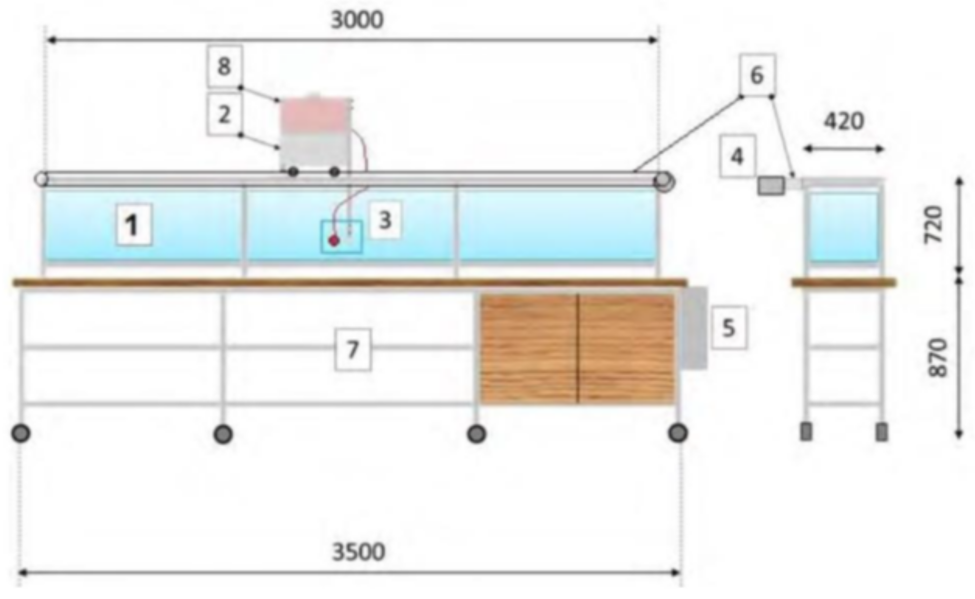
- Ink injection in waterDue to their simplicity, low cost, and conceptual clarity, ink injection in water were among the first techniques to be carried out in this field of science. Despite their simplicity, these tests allow the study of several relevant phenomena in fluid mechanics, and although they are purely qualitative and need to be accompanied by various numerical results, these processes provide great consistency to a study. They are generally performed with laminar flow, as turbulence does not allow clear and differentiable fluid patterns to be created. The dye used must be soluble in water, have a controlled density, and have a value very similar to that of water, with a clearly distinguishable color during the test. Another advantage of this procedure compared to those carried out in a wind tunnel is the great simplicity and low cost of the infrastructure. A wind tunnel requires tolerances that are far above the requirements required to build a water channel. Additionally, a water channel can have a laminar flow of water with two large tanks, where the tests with models are performed statically, or it can be a simple water channel, where the model moves through a static fluid with the help of a trolley; that is, a towing tank. The latter prototype was available in the laboratory where the tests for this article were carried out.To implement this method, a water channel (water towing tank—WTT) located at the School of Aeronautics and Space Engineering (ETSIAE-UPM) was used. Figure 3 shows a sketch of this channel, with all its measures. The channel (1 in Figure 3) was a rectangular prism made of methacrylate, with dimensions of 3000 mm in length, 720 mm in height, and 420 mm in width, and it maintained a velocity of 0.027 m/s for the experiments (Table 1). The models were connected to the trolley by a mobile structure (3 in Figure 3) that could obtain a three-axis adjustment, allowing them to be placed in the correct orientation for each case.Figure 3. Simplified depiction of the water towing tank, including dimensions in mm and the main elements. The parts in the Figure are: channel (1), trolley (2), airfoil (3), engine (4), engine control box (5), belt (6), storage space (7) and ink reservoir (8).Figure 3. Simplified depiction of the water towing tank, including dimensions in mm and the main elements. The parts in the Figure are: channel (1), trolley (2), airfoil (3), engine (4), engine control box (5), belt (6), storage space (7) and ink reservoir (8).
 In order to take pictures during the test, two cameras were used. The lateral images were taken using a AF-S NIKKOR 18–140 mm VR, using a steady position (with a static and robust tripod). The tripod was located at the same point for every test, taking the pictures when the model arrived at that part of the channel.
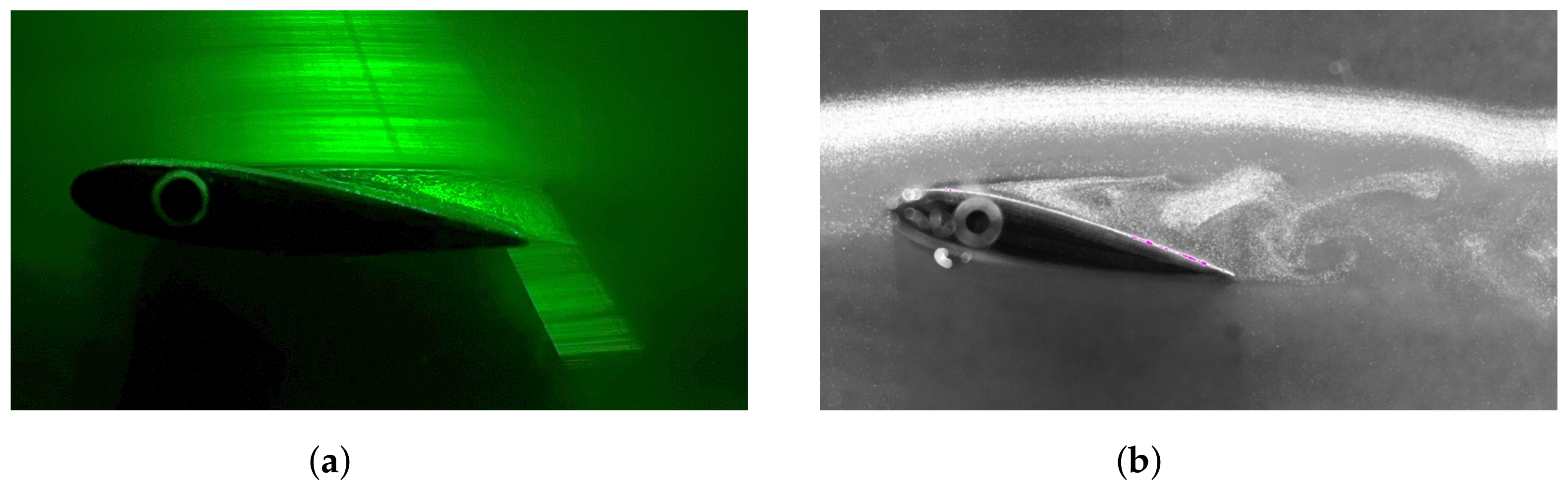
 - Particle Image Velocity in airParticle image velocimetry (PIV) is a technique dedicated to measuring the flow velocity field [22]. It was introduced in the 1990s, and it continues to be developed. It typically combines a double-pulsed laser with a specialized digital camera with a synchronization system. It is considered an appropriate method for indoor airflow investigations, since it is a non-intrusive technique, but it has inconveniences [23]. If the airfoil is not transparent, there is a light-obstruction problem, because the optical paths are blocked; however, if the airfoil is transparent, there can be distortion of the particles’ images. The PIV technique is based on measuring the velocity of tracer particles [24,25] that are transported by the fluid. To achieve this, a pulsed laser is used to illuminate the plane of the fluid being studied, which is generated using a light sheet and suitable optics. The particles are illuminated twice with a laser light sheet. With the correlation of these two pictures, the particle displacement can be calculated. With the following equation, the velocity can be obtained:Finally, a visual layout of the PIV is shown in the following Figure 4:Figure 4. PIV light shot on the test section.
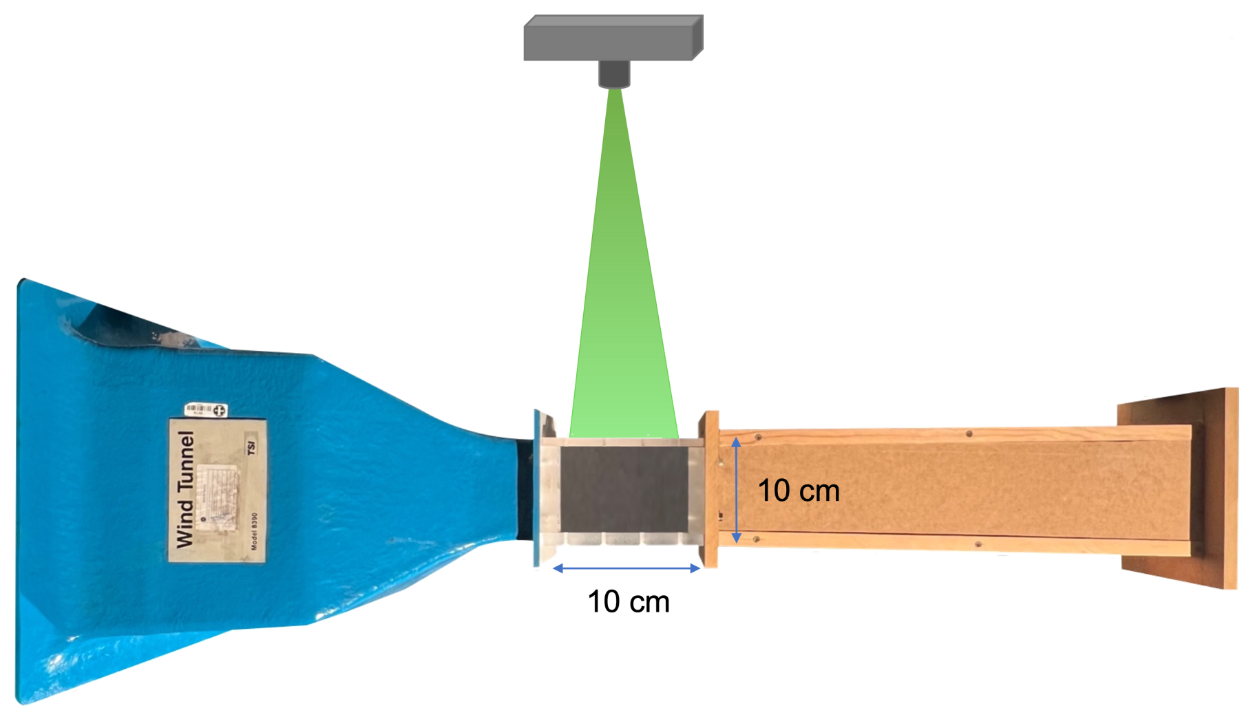
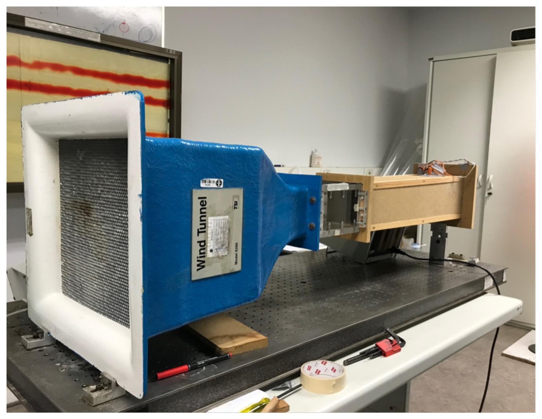
 The experiments with this method were carried out at the Experimental Aerodynamics Laboratory of the National Institute for Aerospace Technology (INTA) with a modified wind tunnel based on a commercial wind tunnel (TSI model 8390) [26]. This is an open-circuit wind tunnel with a closed test section with a square cross-section of 100 × 100 , whose acrylic walls allow visual access. In its original version, the tunnel could reach a speed of 45 m/s. However, the tunnel used was a modification of the original version, aimed at obtaining very low air speeds and low turbulence conditions.The modified tunnel (LSWT) was made up of a new wooden DM diffuser, to properly accommodate the new fan, which offered a lower pressure increase due to its lower speed, allowing the generation of very low Reynolds numbers.The following Figure 5 shows the modified wind tunnel in which all the tests were carried out.Figure 5. Main view of the low speed wind tunnel.
 The study in the low speed wind tunnel (LSWT) was carried out using a commercial 2D-PIV system from TSI Inc. (Thermo Systems, Incorporated-USA) and the licensed processing software INSIGHT 3G. The illumination was based on two Nd:YAG (Neodymium: Yttrium Alluminium Garnet) pulsed lasers that delivered a maximum energy of 190 mJoule/pulse and a CCD camera with frame-straddling.


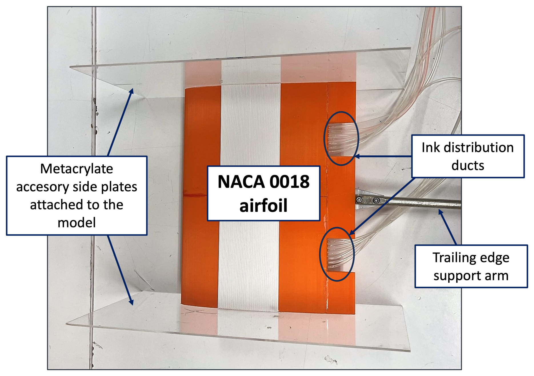
- Water Towing Tank (WTT)To test the airfoil in the water channel, the model was assembled by connecting the distribution system of tubes to the exit hole of the Mariotte Bottle and to the tubes attached to the trailing edge of the airfoil. Two methacrylate side walls were screwed to the sides of the airfoil, to minimize the 3D effects of the flow, and the airfoil was fastened to the trailing edge support arm (Figure 7). The ink distribution ducts were vented by injecting water into the circuit, until it came out of all the leading edge holes, and the main duct was quickly connected to the ink outlet. After the remaining air was removed, the channel was filled and the airfoil was submerged.Figure 7. Detail of the prototype with attached side walls, distribution tubes, and trailing edge support arm.Figure 7. Detail of the prototype with attached side walls, distribution tubes, and trailing edge support arm.
 The camera was placed to capture the flow visualization. The angle of attack of the airfoil was set using a level, and the profile was brought to the center area of the channel. The Nikon lens was focused on the leading edge, and the test began after allowing 5 min for the water to calm down. The main features of the pictures were a focal distance of 18 mm, f/, exposure time 1/20 s; for all experiments, due to the extremely low speed of the trolley, it was possible to obtain more than 30 images in a short period of time; that is, in one minute. Finally, tests were carried out at a Reynolds number of 5500 (Table 1) for angles of attack from 0 to 10.
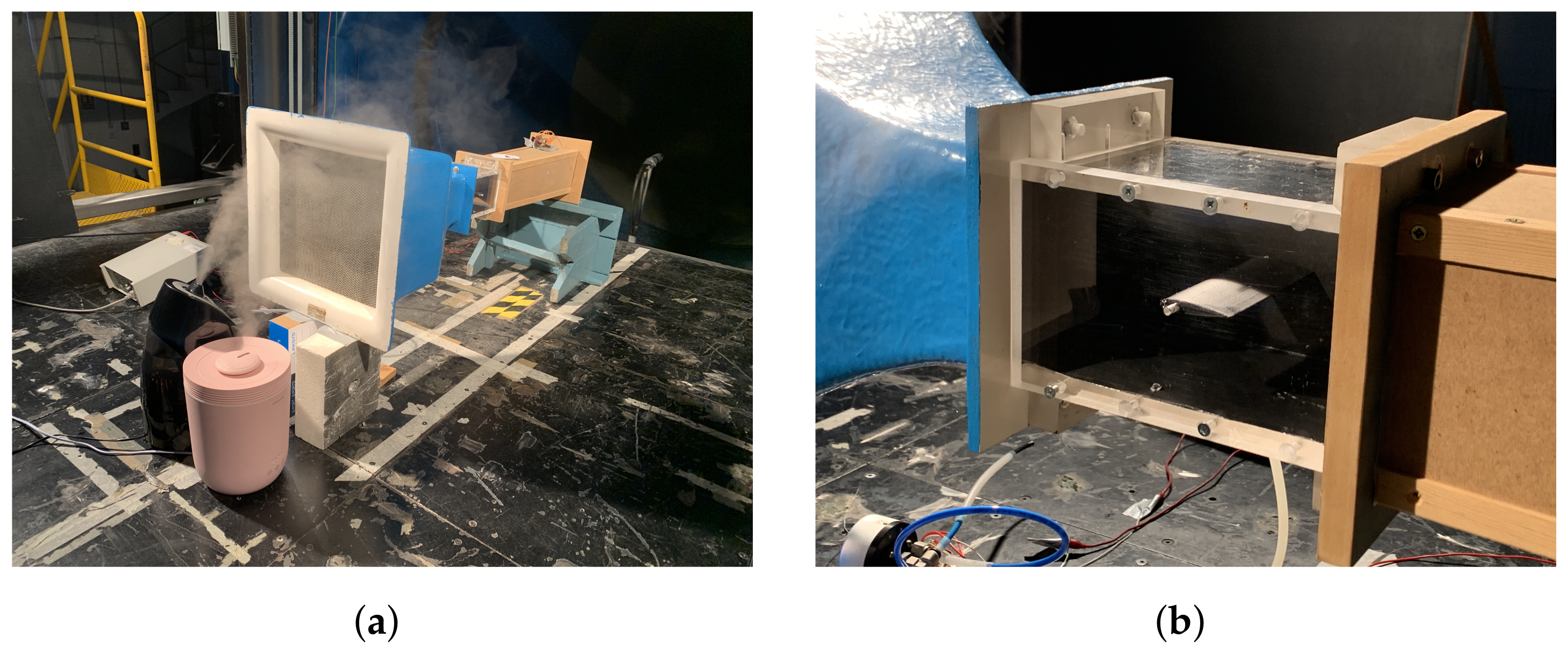
 - Low Speed Wind Tunnel (LSWT)In this case, the model was placed (Figure 8b) using a rod that went from left to right in 25% of the chord (c/4). The next step was to prepare the tracer particles. With oil, there was a spray that threw the particles, but with water, the humidifiers were placed near the entrance of the tunnel (Figure 8a). A camera (PowerView 4M Plus or Iphone 13 Pro Max) was placed on the side of the tunnel to capture the visualization of the flow. The picture properties were a focal distance of 5.7 mm, f/1.5, and exposure time 1/436 s. The angle of attack was changed before the laser started up, from 0 to 12, and the experiments were conducted with a Re = 5500.

3. Results
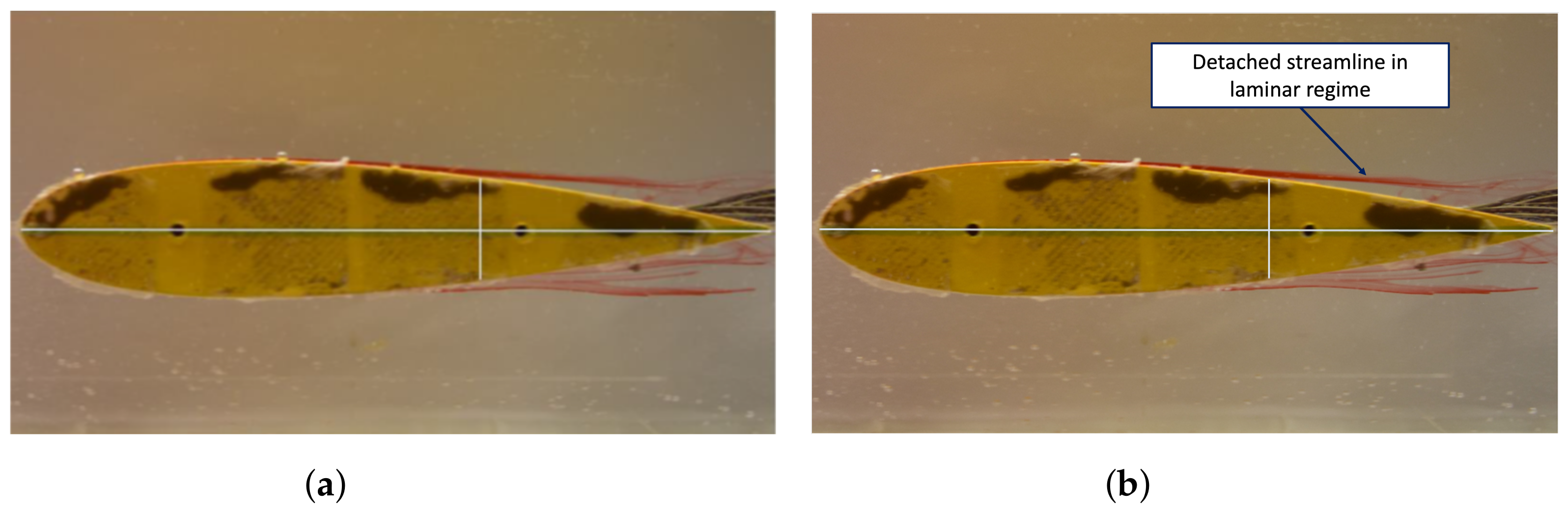
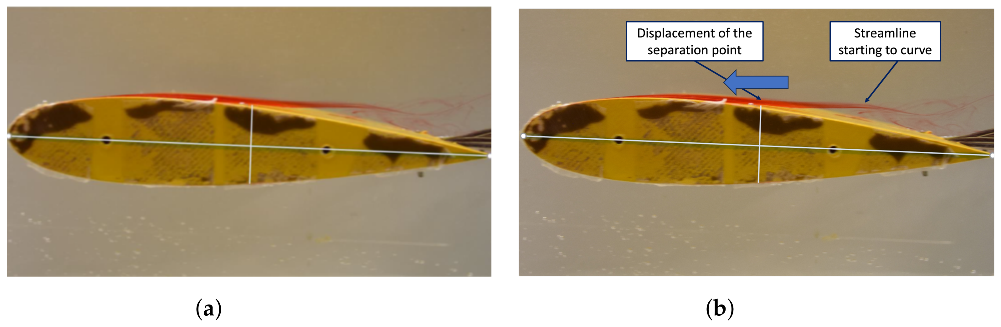
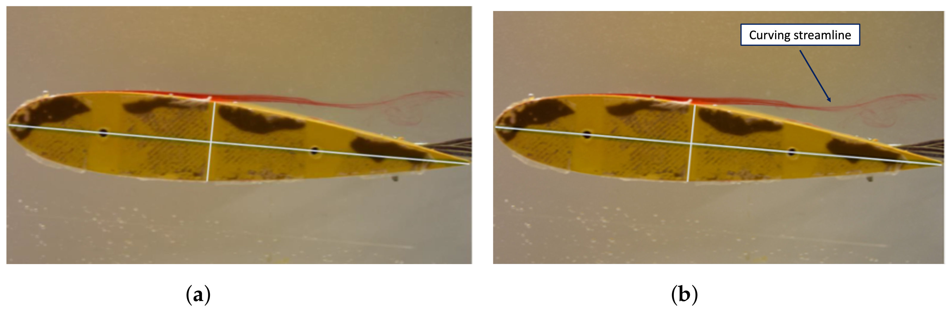
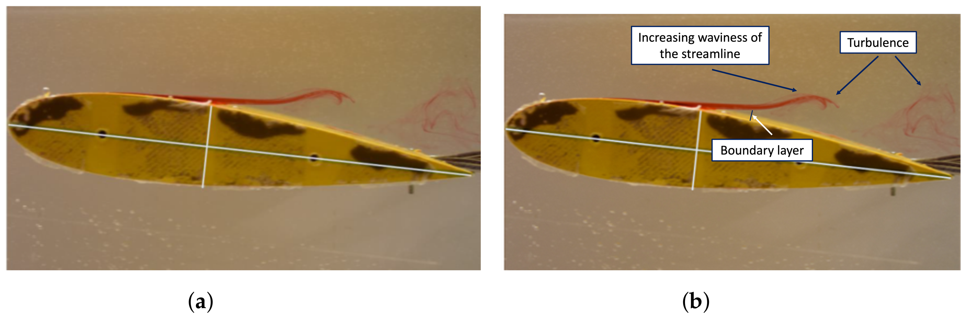
3.1. Water Towing Tank (WTT) Experiments
3.2. Low Speed Wind Tunnel (LSWT) Experiments


4. Conclusions
- Not all visualization techniques have the ability to visualize and explain in detail phenomena such as the flow separation point, boundary layer thickness, recirculation bubbles, vortices downstream of the airfoil, and the onset of turbulence;
- Oil tracer particle visualization in a wind tunnel allows a proper analysis of the recirculation bubble (Figure 19);
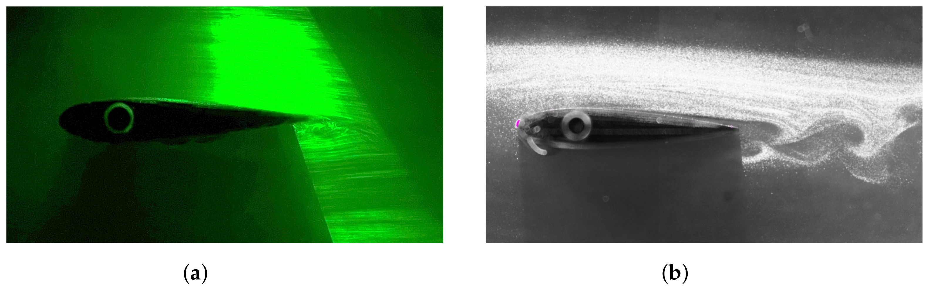
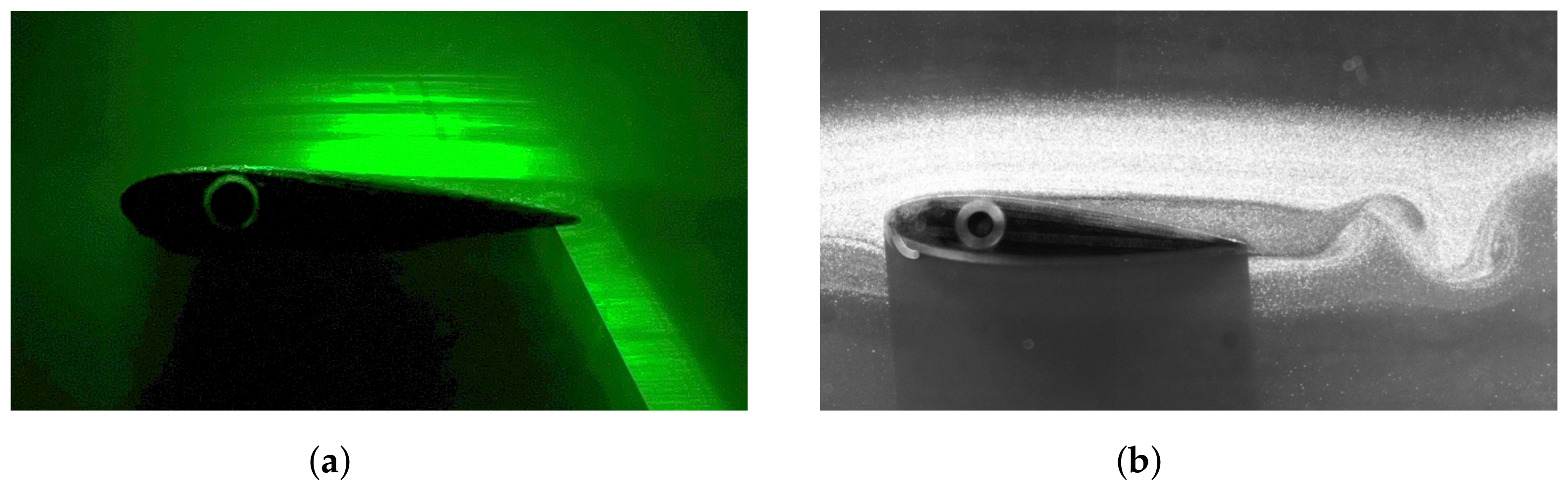
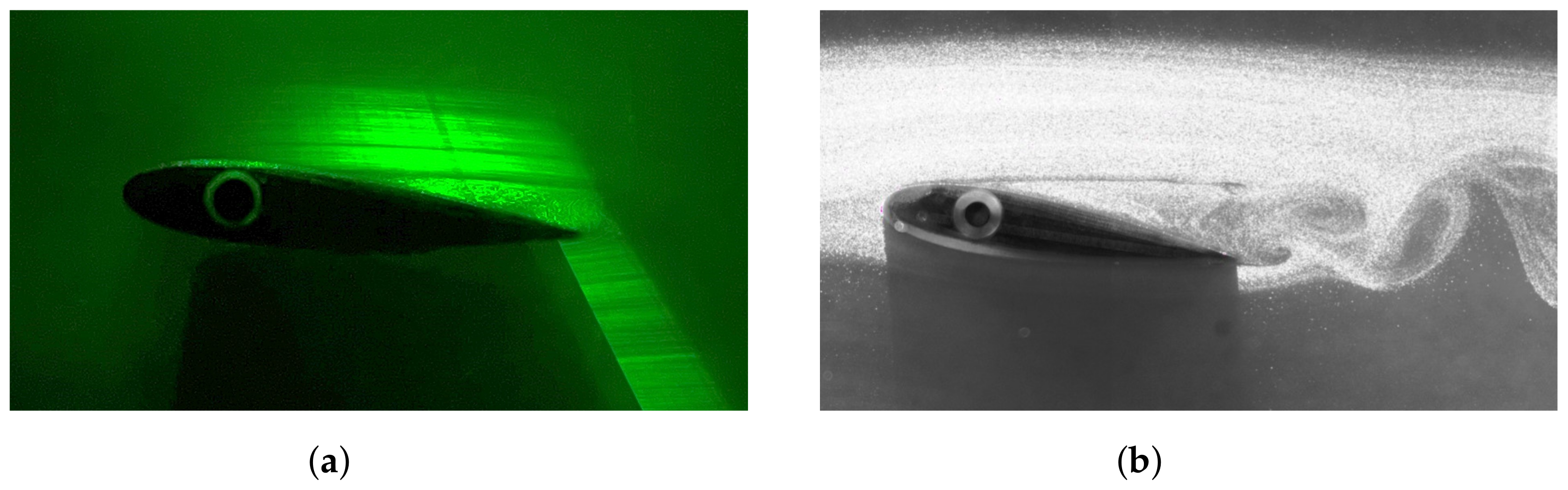
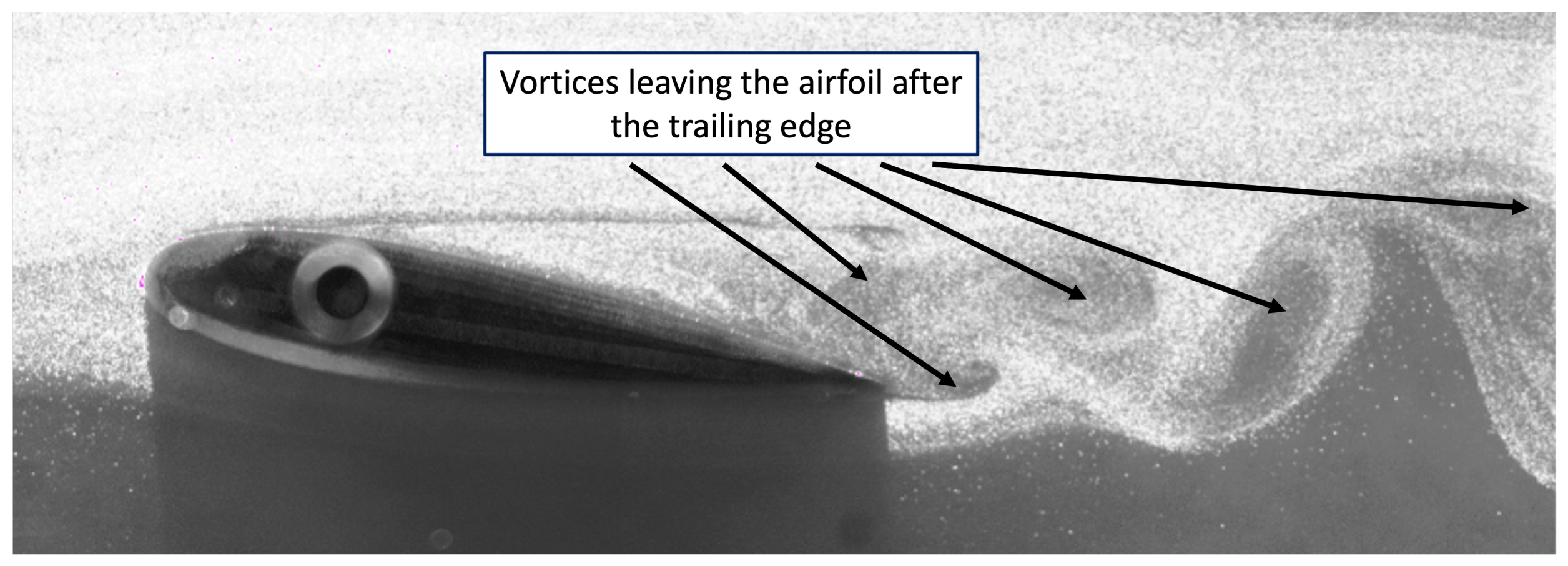
- Water particle visualization in a wind tunnel allows easier visualization of vorticity (Figure 20), although it does not follow the same trend as the other two techniques, due to the particle size argument explained;
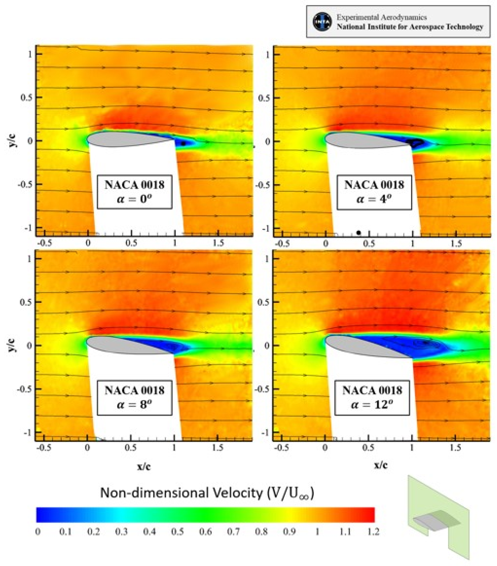
- The PIV technique is suitable for reliable velocity mapping with a small error (Figure 21);
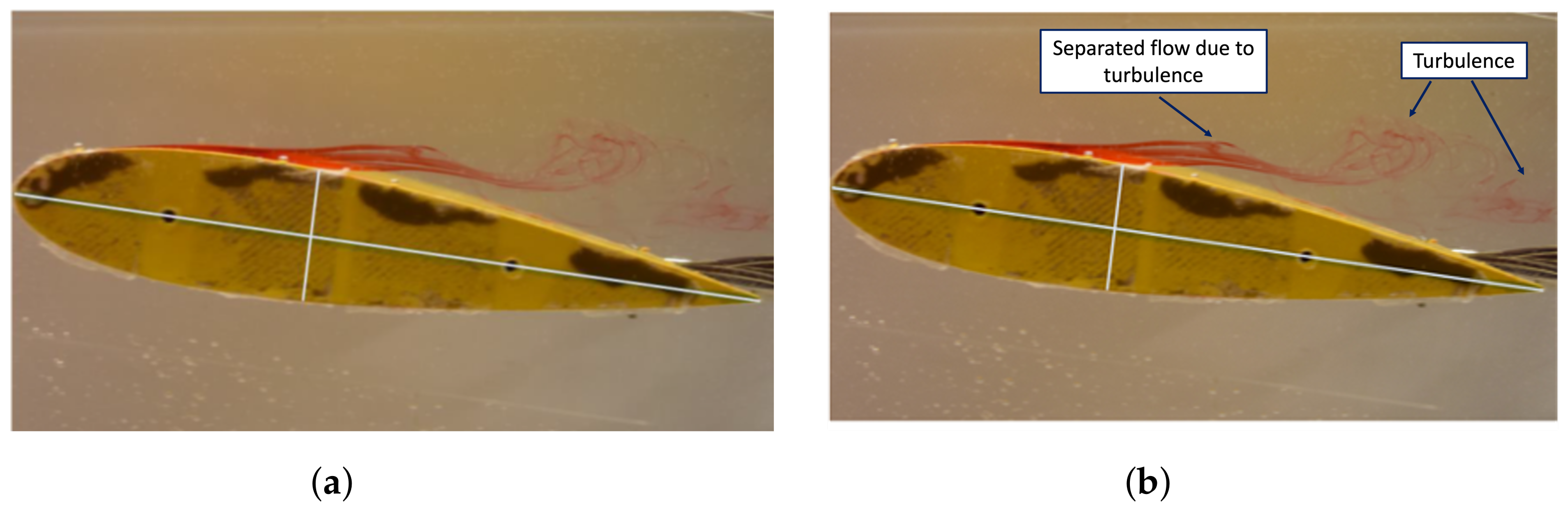
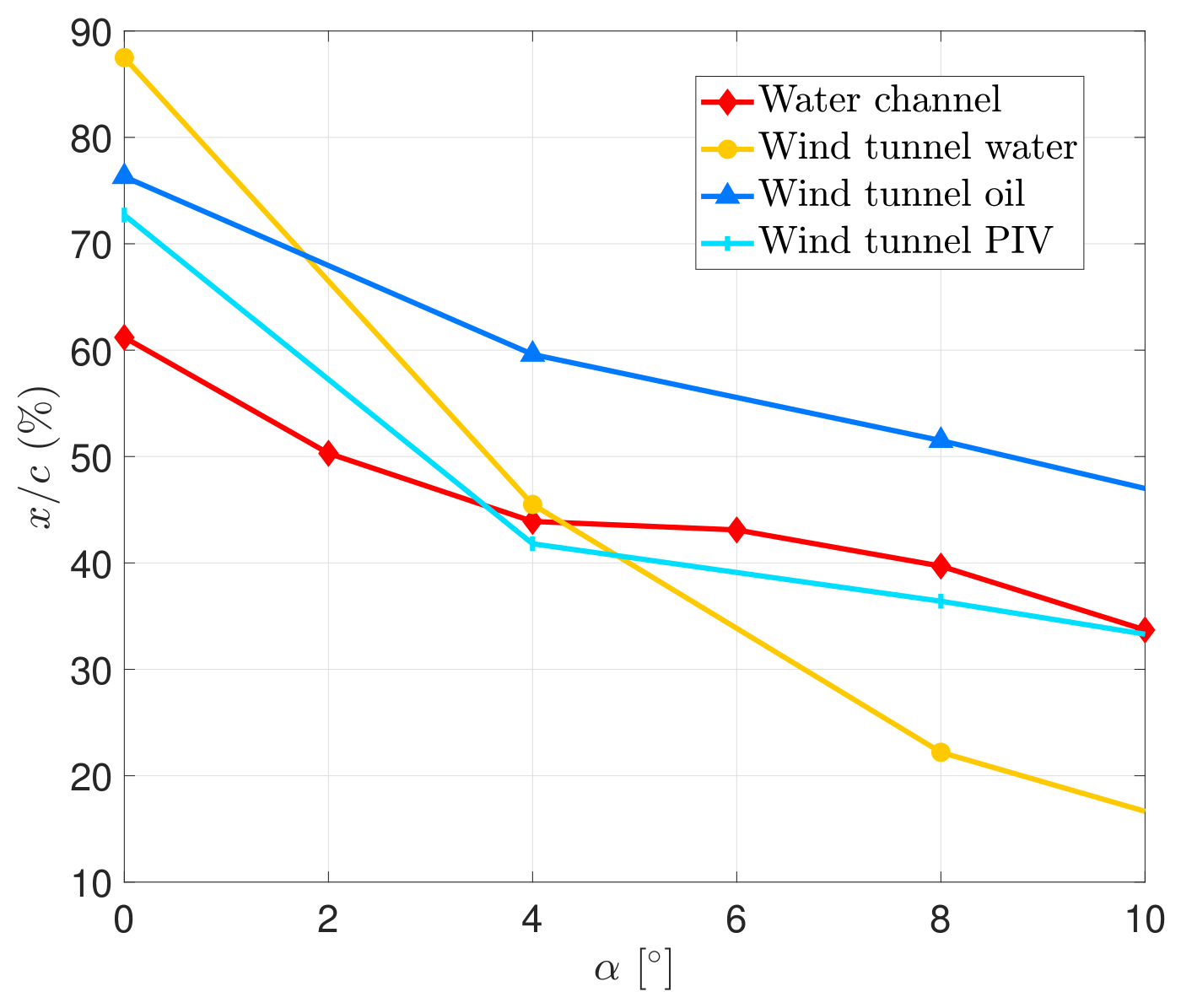
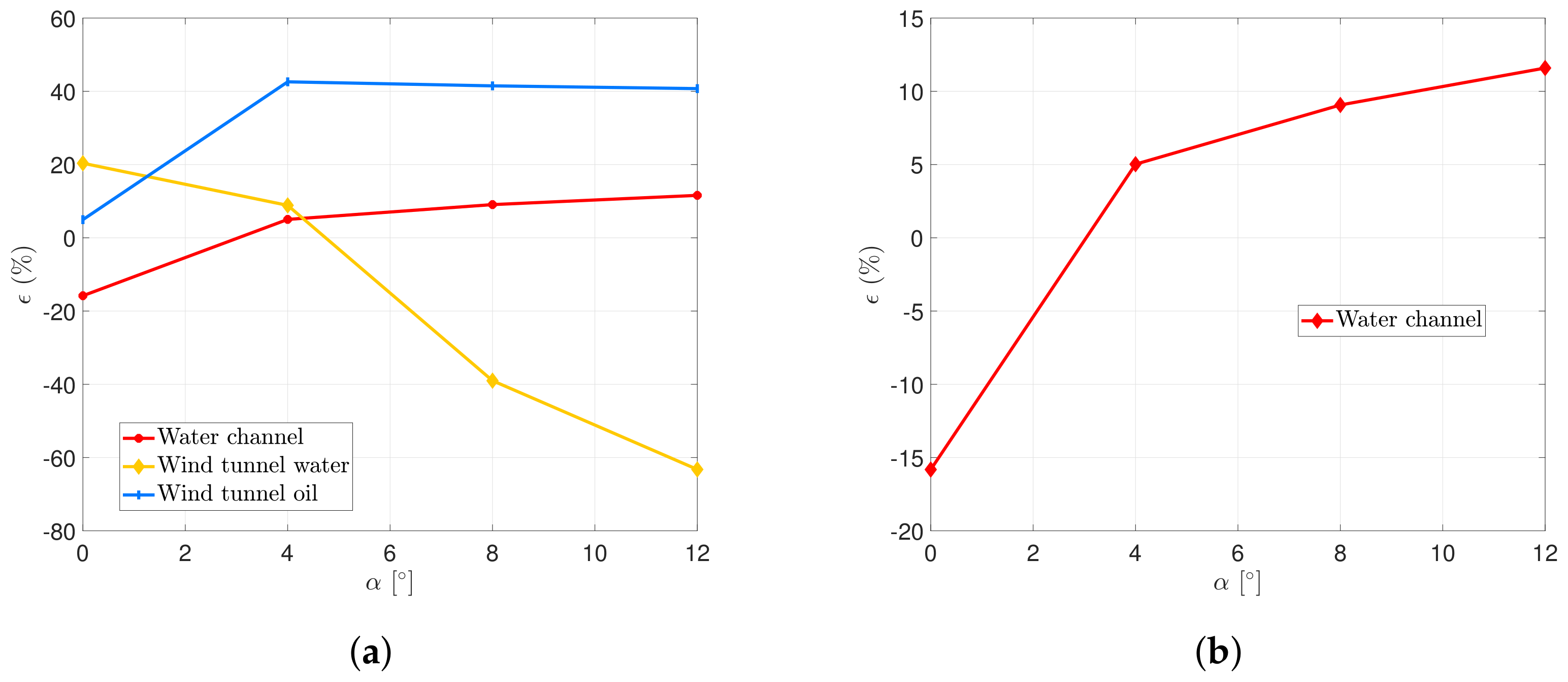
- The water visualization technique (WTT) shows a very similar trend to PIV (Figure 23b), ensuring the validity of the results, although it may not achieve the same level of accuracy. This validates the results obtained in the water channel, which represents the lowest equipment costs among the techniques.
Author Contributions
Funding
Data Availability Statement
Conflicts of Interest
Abbreviations
| LSWT | Low Speed Wind Tunnel |
| MAVs | Micro Air Vehicles |
| NACA | National Advisory Committee for Aeronautics |
| PIV | Particle Image Velocimetry |
| WTT | Water Towing Tank |
References
- Barcala-Montejano, M.A.; Rodríguez-Sevillano, A.A.; Delgado-Obrero, C. Visualization in a water channel as a preliminary design tool. In Proceedings of the 5th European Conference for Aeronautics and Space Sciences (EUCASS), Munchen, Germany, 1–5 July 2013. [Google Scholar]
- Tietjens, O.K.G.; Prandtl, L. Applied Hydro-and Aeromechanics: Based on Lectures of L. Prandtl; Courier Dover Publications: Mineola, NY, USA, 1957; Volume 2. [Google Scholar]
- Clayton, B.R.; Massey, B.S. Flow visualization in water: A review of techniques. J. Sci. Instruments 1967, 44, 2. [Google Scholar] [CrossRef]
- Werle, H. Hydrodynamic flow visualization. J. Annu. Rev. Fluid Mech. 1973, 5, 361–386. [Google Scholar] [CrossRef]
- Gursul, I.; Taylor, G.; Wooding, C.L. Vortex flows over fixed-wing micro air vehicles. Am. Inst. Aeronaut. Astronaut. 2002. [Google Scholar]
- Ballesteros Grande, L.; Martínez García-Rodrigo, L.; Cervigón Corraliza, S.; Eusa López de Murillas, P.; Astudillo Andrés, A.; Casati Calzada, M.J.; Rodríguez Sevillano, A.A. Entrada en pérdida de perfiles NACA a números de Reynolds extremadamente bajos: La aerodinámica en Marte. In Proceedings of the I Semana Interdisciplinar del Espacio y IV Congreso de Ingeniería Espacial, 20–24 June 2022; Available online: https://www.eiecongress.com/programa-completo (accessed on 9 May 2023).
- Kunz, P.J. Aerodynamics and Design for Ultra-Low Reynolds Number Flight; Stanford University: Stanford, CA, USA, 2003. [Google Scholar]
- Crivellini, A.; D’Alessandro, V.; Di Benedetto, D.; Montelpare, S.; Ricci, R. Study of laminar separation bubble on low Reynolds number operating airfoils: RANS modelling by means of an high-accuracy solver and experimental verification. J. Phys. Conf. Ser. 2014, 501, 12024. [Google Scholar] [CrossRef]
- Rodríguez-Sevillano, A.A.; Casati-Calzada, M.J.; Bardera-Mora, R.; Feliz-Huidobro, A.; Calle-González, C.; Fernández-Antón, J. Flow Study on the Anemometers of the Perseverance Based on Towing Tank Visualization. Appl. Mech. 2022, 3, 1385–1398. [Google Scholar] [CrossRef]
- Mateescu, D.; Abdo, M. Aerodynamic analysis of airfoils at very low Reynolds numbers. In Proceedings of the 42nd AIAA Aerospace Sciences Meeting and Exhibit, Reno, NV, USA, 5–8 January 2004; Available online: https://arc.aiaa.org/doi/abs/10.2514/6.2004-1053 (accessed on 9 May 2023).
- Kunz, P.J.; Kroo, I.M. Analysis, Design, and Testing of Airfoils for Use at Ultra Low Reynolds Numbers; American Institute of Aeronautics and Astronautics, Inc.: Reston, VA, USA, 2001. [Google Scholar]
- Koning, W.J.F.; Romander, E.A.; Johnson, W. Low Reynolds Number Airfoil Evaluation for the Mars Helicopter Rotor. In Proceedings of the AHS International 74th Annual Forum & Technology Display, Phoenix, AZ, USA, 15–17 May2018. [Google Scholar]
- Koning, W.J.F.; Johnson, W. Improved Mars Helicopter Aerodynamic Rotor Model for Comprehensive Analyses. AIAA J. 2019, 57, 3969–3979. [Google Scholar] [CrossRef]
- Koning, W.J.F. Airfoil Selection for Mars Rotor Applications. U.S. Patent No. NASA/CR—2019–220236, July 2019. [Google Scholar]
- Johnson, W.; Withrow-Maser, S.; Young, L.; Malpica, C.; Koning, W.J.F.; Kuang, W.; Fehler, M.; Tuano, A.; Chan, A. Mars Science Helicopter Conceptual Design. U.S. Patent No. NASA/TM—2020–220485, March 2020. [Google Scholar]
- Durgesh, V.; Johari, H.; Garcia, E. Aerodynamic behavior and flow visualization on canonical NACA airfoils at low Reynolds number. Vis. Soc. Jpn. 2023, 26, 795–814. [Google Scholar] [CrossRef]
- Winslow, J.; Otsuka, H.; Govindarajan, B.; Chopra, I. Basic Understanding of Airfoil Characteristics at Low Reynolds Numbers (104–105). J. Aircr. 2018, 55, 1050–1061. [Google Scholar] [CrossRef]
- Sun, Q.; Boyd, I.D. Flat-Plate Aerodynamics at Very Low Reynolds Number; Cambridge University Press: Cambridge, UK, 2003. [Google Scholar]
- Bardera, R.; Garcia-Magariño, A.; Sor, S.; Urdiales, M. Mars 2020 Rover Influence on Wind Measurements at Low Reynolds Number. J. Spacecr. Rocket. 2019, 56, 1107–1113. [Google Scholar] [CrossRef]
- Mahbub Alam, M.; Zhou, Y.; Yang, H.X.; Guo, H.; Mi, J. The Ultra-Low Reynolds Number Airfoil Wake; Springer: Berlin/Heidelberg, Germany, 2009. [Google Scholar]
- Samson, A.; Sarkar, S. An experimental investigation of a laminar separation bubble on the leading edge of a modelled aerofoil for different Reynolds number. J. Mech. Eng. Sci. 2015, 230, 2208–2224. [Google Scholar] [CrossRef]
- Persoons, T. Chapter Two—Measuring flow velocity and turbulence fields in thermal sciences using particle image velocimetry: A best practice guide. Adv. Heat Transf. 2022, 54, 37–87. [Google Scholar] [CrossRef]
- Goodfellow, H.; Wang, Y. Industrial Ventilation Design Guidebook; Elsevier: Amsterdam, The Netherlands, 2021. [Google Scholar]
- Lindken, R.; Burgmann, S. Laser-Optical Methods for Transport Studies in Low Temperature Fuel Cells; Elsevier: Amsterdam, The Netherlands, 2012. [Google Scholar]
- Rodi, W.; Laurence, D. Engineering Turbulence Modelling and Experiments 4; Elsevier: Amsterdam, The Netherlands, 1999. [Google Scholar]
- TSI Inc. Model 8390 Bench Top Wind Tunnel P/N 1980004 Rev C; TSI Inc.: Saint Paul, MN, USA, 1989. [Google Scholar]
- Abbot, I.H.; Von Doenhoff, A.E. Theory of Wing Sections Including a Summary of Airfoil Data; Courier Corporation: North Chelmsford, MA, USA, 1949. [Google Scholar]
- Ramirez, A.S.; Marcos, M.E.I.; Haro, F.B.; D’Amato, R.; Sant, R.; Porras, J. Application of FDM technology to reduce aerodynamic drag. Rapid Prototyp. J. 2019, 25, 781–791. [Google Scholar] [CrossRef]
- Szwedziak, K.; Łusiak, T.; Bąbel, R.; Winiarski, P.; Podsędek, S.; Doležal, P.; Niedbała, G. Wind Tunnel Experiments on an Aircraft Model Fabricated Using a 3D Printing Technique. J. Manuf. Mater. Process. 2021, 6, 12. [Google Scholar] [CrossRef]


| Environment | Velocity (m/s) | Typical Length (m) | Dynamic Viscosity (Ns/m) | Density (kg/m) | Reynolds Number |
|---|---|---|---|---|---|
| Mars | 10 | 0.28 | 9.82 × 10 | 1.9 × 10 | 5500 |
| Ink injection in water | 2.7 × 10 | 0.20 | 1.00 × 10 | 10 | 5500 |
| Particle Image Velocimetry in air | 2 | 0.04 | 1.78 × 10 | 1.22 | 5500 |
| Testing | Chord Length (mm) | Wingspan (mm) | Material |
|---|---|---|---|
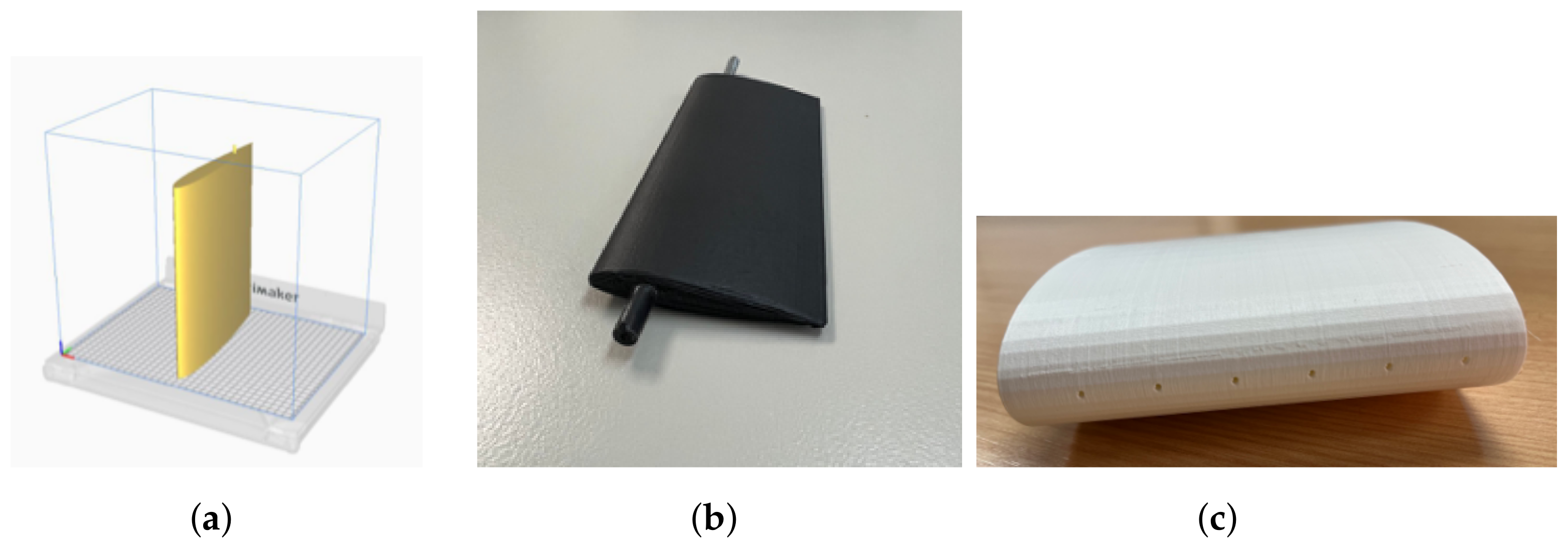
| Water channel | 200 | 250 | PLA (Polylactic acid) |
| Wind tunnel | 40 | 100 | PLA (Polylactic acid) |
Disclaimer/Publisher’s Note: The statements, opinions and data contained in all publications are solely those of the individual author(s) and contributor(s) and not of MDPI and/or the editor(s). MDPI and/or the editor(s) disclaim responsibility for any injury to people or property resulting from any ideas, methods, instructions or products referred to in the content. |
© 2023 by the authors. Licensee MDPI, Basel, Switzerland. This article is an open access article distributed under the terms and conditions of the Creative Commons Attribution (CC BY) license (https://creativecommons.org/licenses/by/4.0/).
Share and Cite
Rodríguez-Sevillano, Á.A.; Casati-Calzada, M.J.; Bardera-Mora, R.; Ballesteros-Grande, L.; Martínez-García-Rodrigo, L.; López-Cuervo-Alcaraz, A.; Fernández-Antón, J.; Matías-García, J.C.; Barroso-Barderas, E. Exploring the Effectiveness of Visualization Techniques for NACA Symmetric Airfoils at Extremely Low Reynolds Numbers. Fluids 2023, 8, 207. https://doi.org/10.3390/fluids8070207
Rodríguez-Sevillano ÁA, Casati-Calzada MJ, Bardera-Mora R, Ballesteros-Grande L, Martínez-García-Rodrigo L, López-Cuervo-Alcaraz A, Fernández-Antón J, Matías-García JC, Barroso-Barderas E. Exploring the Effectiveness of Visualization Techniques for NACA Symmetric Airfoils at Extremely Low Reynolds Numbers. Fluids. 2023; 8(7):207. https://doi.org/10.3390/fluids8070207
Chicago/Turabian StyleRodríguez-Sevillano, Ángel Antonio, María Jesús Casati-Calzada, Rafael Bardera-Mora, Lucía Ballesteros-Grande, Lucía Martínez-García-Rodrigo, Alejandra López-Cuervo-Alcaraz, Jaime Fernández-Antón, Juan Carlos Matías-García, and Estela Barroso-Barderas. 2023. "Exploring the Effectiveness of Visualization Techniques for NACA Symmetric Airfoils at Extremely Low Reynolds Numbers" Fluids 8, no. 7: 207. https://doi.org/10.3390/fluids8070207
APA StyleRodríguez-Sevillano, Á. A., Casati-Calzada, M. J., Bardera-Mora, R., Ballesteros-Grande, L., Martínez-García-Rodrigo, L., López-Cuervo-Alcaraz, A., Fernández-Antón, J., Matías-García, J. C., & Barroso-Barderas, E. (2023). Exploring the Effectiveness of Visualization Techniques for NACA Symmetric Airfoils at Extremely Low Reynolds Numbers. Fluids, 8(7), 207. https://doi.org/10.3390/fluids8070207