Abstract
A wide range of commercial powdered products are manufactured by spray drying emulsions. Some product properties are dependent on the oil droplet size, which can be affected by fluid mechanics inside the spray nozzle. However, most of the key flow parameters inside the nozzles are difficult to measure experimentally, and theoretical estimations present deviations at high shear rates and viscosities. Therefore, the purpose of this study was to develop a computational model that could represent the multiphase flow in pressure swirl nozzles and could determine the deformation stresses and residence times that oil droplets experience. The multiphase flow was modelled using the Volume-of-Fluid method under a laminar regime. The model was validated with experimental data using the operating conditions and the spray angle. The numerically calculated shear stresses were found to provide a better prediction of the final oil droplet size than previous theoretical estimations. A two-step breakup mechanism inside of the nozzle was also proposed. Additionally, some of the assumptions used in the theoretical estimations could not be confirmed for the nozzles investigated: No complete air core developed inside of the nozzle during atomization, and the shear stress at the nozzle outlet is not the only stress that can affect oil droplet size. Elongation stresses cannot be neglected in all cases.
1. Introduction
The spray drying of emulsions is a popular technique that can produce large quantities of low-moisture and high-bulk-density food powders and microcapsules. It can be applied in the fabrication of a wide range of commercial products: infant formula, dairy powders, and encapsulated lipid-soluble colorants and flavors, amongst others [1]. The process begins with the atomization of the liquid emulsion into small droplets. These droplets are then dried into the powdered product by subjecting them to a hot air current [2]. In food application, the continuous phase of the emulsion usually contains carbohydrates, such as maltodextrin [3], that encapsulate the oil droplets in a solid matrix as the water evaporates. This matrix acts like a barrier, and it protects the oil against oxidation or leakage during storage [4].
For the spray drying of food products, pressure swirl nozzles are the most common type of atomizer utilized [5]. In a pressure swirl nozzle, the liquid is fed at high pressures through tangential inclined inlets into a swirl chamber. The angle and location of the inlets induce a rotational, or swirl, flow in the liquid inside of the chamber. While the liquid flows into the nozzle outlet, it accelerates and forms a liquid film, which builds an air core in the center of the swirl chamber [6] (pp. 71–104). Once the liquid film exits the atomizer, it spreads into a conical hollow sheet, which ruptures into small droplets, forming the spray [7].
It has long been reported that the deformation stresses that occur during the atomization can lead to oil droplet breakup [8,9]. To model this droplet breakup, Taboada et al. [4] proposed a way to estimate the maximum shear rate inside of the nozzle based on the critical capillary number for laminar flows. They also established a correlation between this estimated maximum shear rate and the maximum oil droplet size (x90,3) obtained after the atomization [9]. This model is based on some simplifications and assumptions about the flow conditions inside of the nozzle, namely the following:
- There is a complete cylindrical air core inside of the nozzle, which is what enables stable atomization.
- Because of the air core, the liquid forms a thin lamella in the outlet channel, where the oil droplets experience the highest shear rate.
- This highest shear rate determines the maximum oil droplet size that can result from the atomization step.
Taboada et al. [9] reported a good fit of this correlation with the measured droplet sizes, but only for viscosities up to 10 mPa·s and operating pressures up to 10 MPa. For higher values, there seemed to be a deviation from the proposed model, which was an indication that the shear rates were not being calculated properly. The researchers identified that the inviscid approach for the lamella thickness was probably causing the shear stresses to be overestimated. They also concluded that a numerical simulation might provide a more accurate estimation of the shear stresses. Based on that work, the objective of this study was to utilize Computational Fluid Dynamics (CFD) to determine the breakup parameters: most importantly, deformation stress and deformation time. The CFD model had to also be validated with process parameters that could be experimentally measured: the operating pressure/volume flow and the spray angle. The calculated breakup parameters could then be used to establish a better correlation with the measured oil droplet sizes. Additionally, it was our intention to evaluate the validity of the assumptions used for the shear rate estimations from Taboada et al. [4], to find the cause of the deviation.
A variety of studies have developed numerical models of pressure swirl atomizers. Renze [10] and Laurila [11] constructed models in OPENFOAM using an LES turbulence approach, in order to simulate the vorticity and the lamella disintegration during the atomization. Maly [12] analyzed different turbulence approaches in ANSYS Fluent software and found a laminar model could capture the flow conditions of these types of nozzles, since the Reynold numbers are usually below 2200. The studies mentioned focused mostly on determining the discharge coefficient, pressure profile, or spray angle using the numerical models. Renze [10] provided information about the maximum shear and elongation stresses that should be expected inside of the nozzle, but no stress–time profile or further analysis was performed with regard to the stresses. Based on this knowledge, we assembled a numerical model to evaluate how the operating conditions and liquid viscosity affect the oil droplet breakup parameters. We performed this evaluation with two different types of commercial nozzles: the SK nozzle (which is the same one utilized by Taboada et al. [9]) and the MiniSDX nozzle.
2. Nozzle Designs
Two different types of pilot-scaled pressure swirl nozzles were used in this investigation: the SKHN-MFP SprayDry nozzle (referred to as SK) (Spraying Systems Co., Wheaton, IL, USA) and the MiniSDX nozzle (Delavan, Bamberg, SC, USA).
2.1. SK Nozzle
The SK nozzle utilized in this study is shown in Figure 1a. The nozzle is composed of two internal pieces that fit into the outer casing. The top piece has a head with two angled indentations that form the two inlet ports. These two inlet ports can be seen in the bottom view shown in Figure 1b. It can also be seen that the piece has a triangular shaft that fits precisely into the casing (the shaded white ring). This means that there are three slots between the top piece and the casing, which can be seen in Figure 1b as the white spaces between the dark grey and the white pieces. When liquid is pumped into the atomizer, it flows through these three slots and into the two inlet ports. The liquid then continues to the swirl chamber and the outlet channel of the bottom piece, which has an inner funnel shape.
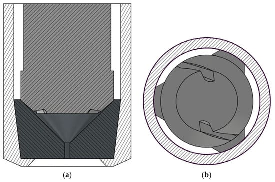
Figure 1.
Geometry of the SK nozzle. (a) Front view of the internal pieces of the nozzle (dark grey and black) surrounded by the white stripe-patterned casing. (b) Bottom view of the top internal piece (dark grey). The casing is illustrated as a stripe-patterned ring.
2.2. MiniSDX Nozzle
The MiniSDX nozzle utilized in this study is shown in Figure 2. The nozzle is composed of two internal pieces that fit into an outer casing. The top piece houses the spirally shaped inlet port and swirl chamber. This piece rests on top of a thick plate (the bottom piece) that has the outlet channel of the nozzle drilled into it. In this case, when the liquid is pumped into the atomizer, it flows into the casing around the top piece (white); it then flows into the inlet port and the swirl chamber. The nozzle exit, located in the center of the swirl chamber, is followed by a conical outlet.
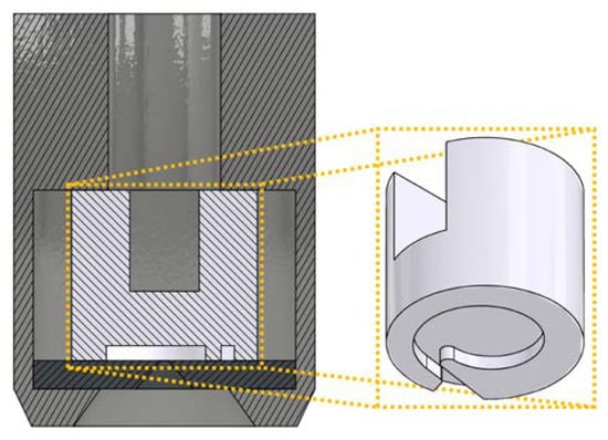
Figure 2.
Geometry of the MiniSDX nozzle. The top piece (white) is shown isolated on the right to give a better view of the spirally shaped inlet port and swirl chamber. The casing (dark grey) and bottom plate (black) are also shown.
3. Experimental Setup
The atomization experiments were carried out following the procedure detailed by Taboada et al. [4], with various model solutions and operating conditions.
3.1. Atomization Rig
The experiments were performed at atomization pressures (pexp) of 5, 10, and 20 MPa at room temperature, which was assumed to average 25 °C for all calculations and simulations. Flow conditions outside the exit orifice of the atomizer were optically analyzed for the spray angle measurements. For that purpose, a high-speed video camera (OS3-V3-S3, Integrated Design Tools Inc., Tallahassee, FL, USA) was used. It was equipped with a 150 mm macro lens (150 mm F2.8 EX DG OS HSM, Sigma, Kawasaki, Japan) with a polarizing filter. The exit orifice of the atomizer was illuminated from the opposite side of the camera with diffused light from a high-performance light-emitting diode system (constellation 120 E, Imaging Solution GmbH, Eningen unter Achalm, Germany).
3.2. Model System
The atomization experiments were performed with a model for oil-in-water emulsions. The model emulsion was prepared according to a procedure similar to the one described by Taboada et al. [4]. The emulsions consisted of medium chain triglyceride oil (MCT oil, WITARIX® MCT 60/40, IOI Oleo GmbH, Hamburg, Germany) as the oil phase, whey protein isolate (WPI, Lacprodan DI-9224, Arla Food Ingredients, Viby J, Denmark) as an emulsifier, and a solution of maltodextrin (MD, Cargill C*DryTM MD 01910, Cargill Deutschland GmbH, Düsseldorf, Germany) with a dextrose equivalent of 14.5 in water as the continuous phase.
To validate the CFD model, we recorded the experimental operating conditions, that is, pressure and volume flow, during the atomization of emulsions of two different viscosities. Each emulsion had an oil content of 1%. This low percentage meant that the viscosity and density of the emulsion and of the continuous phase were virtually the same [9]. Consequently, for the simulations, the emulsions could be modelled as single-phase liquids with the same viscosity and density as the actual emulsion. The properties of these two emulsions are shown in Table 1, along with the properties of the simulated air phase. The properties of air were taken from the database of ANSYS, Inc. [13]. The viscosities of the emulsions were measured with a rotational rheometer (Physica MCR 301, Geometry DG26.7, Anton Paar, Graz, Austria) with shear rates between 10 and 103 s−1. They both presented constant viscosities in this range. The density of emulsions was measured with a tensiometer (DCAT 21, DataPhysics Instruments GmbH, Filderstadt, Germany). All measurements were taken at 20 °C.

Table 1.
Density (ρ) and viscosity (µ) used in the simulations for the analyzed emulsions and the air phase.
The measurement of spray angles was executed in a separate experimental run. The same operating conditions were recreated, but MD solutions without any oil content were used. Because of the low oil concentration in the original emulsions, we considered that the use of MD solutions would not significantly affect the results of the spray cone formation and its angle. The density and viscosity of the solutions were measured and proved to have the same values as the ones shown in Table 1.
3.3. Spray Angle Measurement
The spray angle was determined in a different manner for experiments and simulations. For the experiments, high-speed imaging was used to record the spray cone that formed outside of the nozzles. For each combination of nozzle, viscosity, and operating pressure, ten photos were randomly chosen. Each photo was then divided into its left and right side. Figure 3 shows, as an example, the right half of one of the experimental photos. A line was drawn from the nozzle outlet and along the regions with dense spray mist (seen as dark regions in the photo). The slope of the line determined the spray angle on the right side. The left side of each profile was subjected to the same procedure, and we summed the angles from the left and right side to obtain the spray angle.
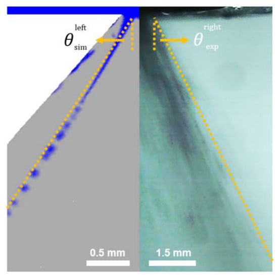
Figure 3.
Example of how the spray angles (θ) were determined in the simulations (left) and the experiments (right). In the simulations, the liquid profile outside of the nozzle is plotted (shown in blue). The orange line represents the measured angle, which follows the profile of the spray cone. Reference scales are provided for both the simulated profile and the experimental image.
For the simulations, the procedure was simpler, since we could obtain a 2D profile directly from STAR-CCM+. An example of a simulated spray cone profile is shown on the left side of Figure 3. Because the profile was much clearer, a line was simply drawn following the path of the liquid lamella, and the angle was determined from the slope of the line. The other side of the image was subjected to the same procedure, and then the two angles were summed to determine the spray angle.
4. Numerical Model
The numerical model was implemented on ANSYS Fluent 2019 R3 software (Ansys, Inc., Canonsburg, PA, USA). Several steps were followed to build the model that best represented the physical system. Different approximations to the governing equations and numerical methods were evaluated based on the literature, in order to select the ones that could better capture the multiphase flow. The simulating and boundary conditions of the model were defined to approximate the experimental conditions. A polyhedral mesh was generated to represent the internal volume of the nozzles.
4.1. Internal Volume of the Spray Nozzles
To simulate the multiphase flow inside of the nozzles, their internal volume was extracted, as shown in Figure 4 for the SK and Figure 5 for the MiniSDX nozzle. The different regions of interest are indicated as well. A large inlet region was included before the regions of interest. This was meant to ensure that the boundary conditions did not artificially affect the simulation results. Additionally, a region outside of the nozzle exit, which we referred to as an airbox, was attached to the nozzle exit. This allowed us to observe the formation of the spray cone and use the spray angle as an additional validation parameter.
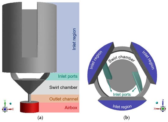
Figure 4.
Sections of the internal volume of the SK nozzle from (a) top view and (b) side view.
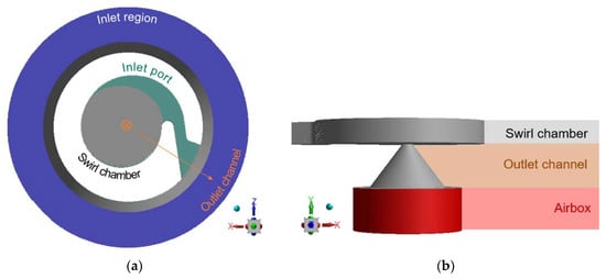
Figure 5.
Sections of the internal volume of the MiniSDX nozzle from (a) top view and (b) side view. The annular inlet region is omitted in the side view; otherwise, it would obscure the swirl chamber from view, since the inlet region surrounds it.
4.2. Governing Equations and Models
The model selection for this investigation was based in the numerical models implemented by Maly et al. [14] and by Laurila et al. [11]. The multiphase flow of the nozzle is an immiscible mixture of air and a liquid phase. Both phases were modelled as Newtonian and incompressible. The assumption of air incompressibility was based on the fact that velocities above 0.3 Mach were not expected inside of the nozzle. This is a commonly mentioned criterion for incompressibility assumptions in the literature [15] (pp. 62–75). The expectation of low Mach numbers is based on the working principle of the nozzle. After all, the air should remain relatively static, while the liquid is the one that swirls, accelerates, and then breaks into droplets. This assumption was also verified later with the simulation results.
The multiphase flow itself was modelled using the Volume Of Fluid (VOF) method. The flow inside, and at the exit of, the nozzles was modelled as transient because of the unstable free interface between the phases, using a first-order implicit formulation. To resolve the interface, we implemented a compressive method, namely CICSAM. The selection of CICSAM was based on previous modelling studies [16,17] as well as the guidelines of ANSYS Fluent [13]. The equations and formulations used by the VOF and CICSAM schemes are described in one of our previous studies [17].
A pressure-based solver was implemented, using the Pressure Implicit with Splitting of Operators (PISO) algorithm for the velocity-pressure coupling. A schematic of the general solver algorithm of this iteration with a VOF formulation is described in [18]. All equations were spatially discretized with a second-order upwind scheme, except for the pressure. For the pressure, we utilized the PREssure Staggering Option (PRESTO!) scheme. All discretization schemes were chosen following recommendations by ANSYS, Inc. [13].
In regards to the flow regime, the flow inside of the pressure swirl nozzles was assumed to be laminar. This assumption was based on two reasons. First, the Reynolds number at the liquid lamella in the nozzle outlet was determined following the formulation commonly used for annular flows [19,20]. The number was calculated at the outlet because that is where the highest velocities are reached. Using the velocity estimations from Taboada et al. [9], we expected a Reynolds number from 1100 to 2200, which would at most barely reach the beginning of the transition regime [21]. Secondly, Maly et al. [14] already performed an extensive comparison between different turbulence modelling options and reported good results with laminar modelling with this type of swirling flow. The flow conditions that they simulated reached Reynolds numbers of up to 1700, which are slightly lower than the maximum expected here; however, it was decided that it was a good guideline for our numerical model.
4.3. Boundary and Simulation Conditions
For both types of nozzles, a mass flow inlet was set at the top of the inlet regions. The decision to fix the inlet mass flow, rather than an inlet pressure, was intended to make the simulations as comparable to the experimental conditions as possible. The operating pressure is measured in the experimental setup at the pump outlet and not where the liquid enters the nozzle. Due to the pressure loss between these points, we do not have accurate pressure values from the nozzle inlet. In comparison, due to mass conserving conditions, one can easily suppose that the mass flow, or rather the volumetric flow, that is measured at the pump outlet is the same as that which enters the nozzle. On the other hand, the nozzle exit was set as an atmospheric pressure outlet.
Gravity was set in the direction of the outlet (the y-direction in Figure 4 and Figure 5b). For the initialization of the simulation, the swirl chamber, outlet channel, and airbox were filled with air, and the inlet port(s) and the inlet region were filled with liquid. An adaptive multiphase-specific time step was used to ensure that the global Courant number was maintained below 1. The method monitors, across all cells in the mesh, the minimum ratio between the respective cell volume and the total outgoing volume flux. This minimum ratio is used as the next time step. It should be noted, however, that ANSYS, Inc. [13] mentions that local Courant values of up to five can be managed by the solver without significantly affecting convergence.
All simulations were run for at least 15 ms. This minimum run-time was decided based on two main criteria. On the one hand, the inlet pressure on all simulation runs stabilized between 4 and 8 ms after initialization. On the other hand, we estimated the time that the liquid would require to flow all throughout the nozzle, which also amounted to 8 ms. Based on this information, we accounted for 8 ms of initialization time and used the other 7–8 ms of simulated time for the analysis. For every time step, the convergence criterion was for the residuals to reach values below 10−3, which was usually achieved within 20 iterations.
4.4. Mesh Generation
The aim of the study was to understand the two-phase flow in the nozzle. The interesting sections for this purpose are downstream from the inlet ports: the swirl chamber, outlet channel, and airbox. To save calculation efforts, only these sections were meshed with a fine polyhedral grid (shown in Figure 6). The cell was also set to half of the reference size in the region near the outlet of the nozzles (see the center darker regions in Figure 6), given that the narrowest section in both nozzles is there. The grid was created in two steps. First, a tetrahedral mesh was established using the patch-conforming method from ANSYS. Then, the mesh was converted to a polyhedral mesh in Fluent, by fusing the tetrahedral cells. Figure 6 shows the final mesh obtained for the two geometries. It should be noted that thin prismatic cells were generated near the wall all around the geometry to better approximate the boundary layer [22].
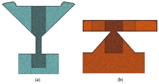
Figure 6.
Plane section of the meshes used to simulate (a) the SK nozzle and (b) the MiniSDX nozzle. The inlet region, which was fitted with a hexahedral mesh, is omitted to facilitate visualization of the sections of interest.
For the inlet regions, part of the volume was mesh with extruded cells, to reduce computational efforts. First, a tetrahedral mesh was created for the bottom 30% of the volume, with 150% as the reference size of the inlet ports. The rest of the volume was fitted with a mesh extruded from these bottom cells. The number of extruded cells along the remaining height of the inlet region was set to 60. Because the cells were extruded from the normal tetrahedral mesh, prism cells were still created to account for the boundary layer near the wall. During the conversion in Fluent, both the base and the extruded cells were transformed accordingly, so that their vertices still matched with each other.
A mesh independence test was carried out to define the optimal cell density. For our case, we used the operating pressure and the velocity profile at the nozzle outlet as convergence criteria. To ease computational time, the mesh test was run with a simplified steady-state single-phase system using the SK nozzle geometry. With that in mind, we simulated the nozzle as completely filled with the maltodextrin solution of 10 mPa·s. Four meshes (M1–M4) were generated using the parameters shown in Table 2. They all differed in reference cell size, while the number of prism layers was kept constant. The thickness of the first layer was calculated following good practice recommendations by White [23] (p. 467). This included making sure that the y+, which is the dimensionless wall distance relative to the viscous wall layer as defined by Schlichting and Gersten [24] (pp. 519–610), was below one. For that calculation, we used the liquid velocities estimated by Taboada et al. [9] for similar process conditions.
Table 2.
Mesh parameters for the four grids (M1–M4) evaluated in the mesh independence test.
Figure 7 shows how the first convergence criterion, pressure, changes with the mesh size, which we characterized in the figure with the number of cells in the entire mesh. As expected, the predicted pressure converges to a stable value as the number of cells increases. From mesh M2 onwards, the variation of the predicted value with the cell number is already below 2%.
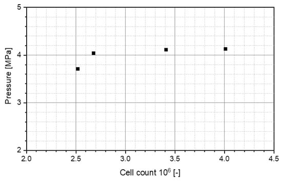
Figure 7.
Effect of the mesh size on the predicted operating pressure of the SK nozzle. All simulations were performed for a viscosity of 10 mPa∙s at QL = 0.35 L/min.
The spatial resolution of the grid was evaluated using the second convergence criterion: the velocity profile at the outlet of the nozzle. The resulting profiles are shown in Figure 8. On the left, the tangential velocity is plotted; on the right, the axial velocity. For the tangential velocity, the behavior of the profiles from M1–M4 correspond with what was observed for the pressure, in that there is very little difference when comparing the meshes from M2 onwards. With respect to the axial velocity, there is a slight dimple in the center of the profile with M2, although it must be mentioned that it represents only a 3.5% difference with the center value obtained with M4. With this in mind, we concluded that M2 was already fine enough to be able to simulate the flow conditions inside of the nozzles.
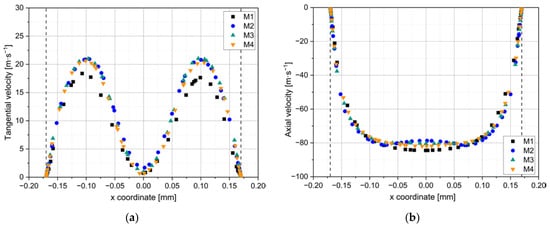
Figure 8.
(a) Tangential and (b) axial velocity profiles across the outlet of the SK nozzle, when simulated at QL = 0.35 L/min with the emulsion of 10 mPa·s. The profiles are shown for four different meshes of increasing size (M1–M4). The radius of the nozzle outlet is indicated as the two vertical dashed lines.
Since the mesh independence test was carried out with a single-phase flow, the mass conservation and interface sharpness for the VOF model could not be evaluated during this step. Nevertheless, two different factors were used in the study to validate the accuracy of VOF during the actual multiphase simulations. On the one hand, the error residuals, which include the continuity equation, were monitored at each time step (as mentioned in Section 4.3). On the other hand, the sharpness of the interface was checked during the spray cone formation analysis (see Section 5.2.1 and Section 5.3.1). While there is an expected smearing of the liquid phase once the spray cone forms (and the liquid lamella thins out), all flow variables are measured inside or directly at the nozzle exit, so this downstream smearing should have no effect on the measured velocities, pressures, or stresses.
4.5. Droplet Parameter Measurements
The final objective of the CFD model was to track the path and the deformation stresses that a droplet would experience as it flows through the nozzles. To be able to do this, we inserted 200 virtual (i.e., massless) point particles at the end of the inlet region of the nozzles at randomized positions. An example of this sample of streamlines is shown in Figure 9 for both nozzles. Each particle would then follow a streamline of the flow, and we recorded the position and residence time of each particle along its path through the nozzle. We used this sample of particles to calculate the residence time distributions for each simulated case.
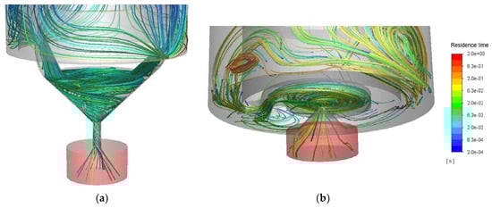
Figure 9.
Examples of the sampled streamlines inside (a) the SK nozzle and (b) the MiniSDX nozzle.
It should be noted that streamlines are integrated from the velocity field of the liquid at a specific instant [13], which for us was after 15 ms of simulation. Because of this integration step, some streamlines are artificially extrapolated outside of the simulated region, which causes the calculation to be aborted for those specific streamlines. This can especially happen at points where there are contractions in the geometry or the phase becomes thinner. Both of these happened in our case near the outlet channel. This effectively means that not all of the 200 streamlines followed the complete path through the nozzle. However, for the residence time, the randomized sampling was repeated to ensure that at least 10 measurements could be taken for each of the sections of interest.
To measure the deformation stresses, three particles were randomly chosen for each nozzle, pressure, and viscosity. In the case of the SK nozzle, we made certain to choose three particles, each from one of the three different inlet surfaces.
We recorded the shear rate and velocity of each particle along its path through the nozzle. With this information, we calculated the shear and elongation stresses following the equations for a Newtonian fluid [25,26]:
where is the shear stress, is the shear rate, is the elongation stress, and is the corresponding elongation rate. The assumption that the elongation, or extensional, viscosity is was corroborated by Grace [27]. The shear rates were calculated directly by Fluent. For the elongation rates, we took advantage of the fact that the droplets were following a streamline. By its definition, the flow velocity of a point in a streamline (s) is always tangential to the streamline [28] (pp. 10–29). At the same time, we can imagine the elongation rate as the rate of change of velocity (us) in the direction of the velocity [29]. Because this direction always overlaps with the streamline, we can calculate the rate as the derivative of the velocity magnitude along the length of the streamline:
where the positive superscript indicates that only the positive part of the derivative is used, since the droplet is only elongated when it is accelerated. We calculated this derivative numerically, with a simple first-order upwind scheme [30] (p. 103). Finally, we calculated the shear stress history (SSH) by integrating the shear stress along the streamline with respect to the particle time. This allowed us to evaluate the effect of the deformation magnitude and the deformation time simultaneously. No stress history was calculated for the elongation stresses, for reasons that will be discussed in Section 5.4.1. By ensuring at least three particles were analyzed for every configuration, we could evaluate whether the tendencies observed in the stresses were caused by the randomly chosen particle or actively caused by the analyzed factors: geometry, viscosity, and pressure.
5. Results
As mentioned before, the main objective of this study was to determine the oil droplet breakup parameters during atomization with the analyzed pressure swirl nozzles (Section 5.4). In order to do that, we first had to validate the prediction of the operating conditions (Section 5.1) and then analyze if the multiphase flow was being simulated correctly by the numerical model (Section 5.2 and Section 5.3). In all cases, the analysis was done for the SK as well as the MiniSDX nozzle.
5.1. Validation of Predicted Operating Conditions
To evaluate the numerical prediction of the flow conditions, we simulated three different operating pressures from the experiments, with two emulsion viscosities for each pressure. The results from experiment and simulation are shown in Figure 10 for SK (left) and MiniSDX (right) nozzles. A “mass flow inlet” was used in most of the simulations, so the mass flow rate was fixed. As the density of the liquid is fixed, this corresponds to a set volumetric flow, which is shown in the figures. The simulated pressure at the inlet was then compared with the experimental data. For the MiniSDX nozzle, it should be noted that no experimental data could be generated for 35 mPa·s at 20 MPa. Therefore, no simulation was performed for these conditions.
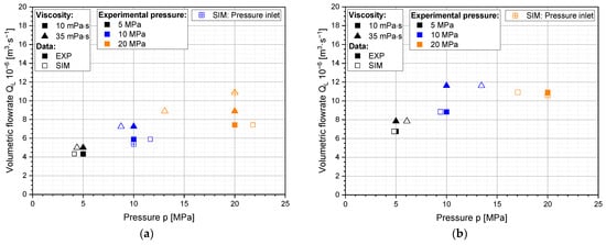
Figure 10.
Experimental (EXP) und simulated (SIM) operating conditions with (a) the SK nozzle and (b) the MiniSDX nozzle for emulsions of 10 und 35 mPa·s. Three experimental pressures were evaluated. The crossed data points were simulated with a set inlet pressure (pressure inlet), while the other simulations were executed with a fixed mass flow (mass flow inlet).
For the SK nozzle, the simulation predicts the operating pressure with an error that ranges between 9% and 35%. The highest error occurs at an experimental pressure of 20 MPa and a viscosity of 35 mPa·s. The average error is 17%. For the MiniSDX, the simulations results in an average error of 15%. The highest error occurs at an experimental pressure of 10 MPa at 35 mPa·s, which is 34%. In contrast, the lowest error observed is 4%, for a pressure of 5 MPa and a viscosity of 35 mPa·s. However, it should be noted that at higher pressures (>10 MPa), some pressure variation is observed in the experimental setup. This variation reaches as high as ±1 MPa at 20 MPa. This can also affect the difference between simulations and experiments.
Additionally, we evaluated some alternative cases with “pressure inlets”, i.e., with a fixed inlet pressure instead of a fixed volume flow, to see if the different boundary condition reduces the numerical error. The three alternative cases are shown in Figure 10 as empty, crossed-out measurement points. In all three cases, the relative error was reduced when the pressure inlet was used instead of the mass flow inlet. For the SK, the 35% error that was initially observed in the pressure prediction (with 35 mPa·s and 20 MPa) was reduced to a 20% difference in the volume flow. For the MiniSDX, the relative error was reduced from 15% to 3%.
To assess the fidelity of the simulation results, we discuss them in the context of similar studies on pressure swirl nozzles. For example, Renze, Heinen, and Schönnherr [10] modelled the atomization of a polymer solution of around 100 mPa·s. They obtained around a 30% difference between the predicted and the experimentally measured pressure drops, although they used LES for the turbulence modelling. Maly et al. [14] used a velocity inlet as a boundary condition. Nonetheless, a velocity and a mass flow inlet are effectively the same condition when the phase is incompressible [13]. They reported no error in their pressure predictions, even when assuming a laminar flow. However, their test liquid was Jet A-1, which has a viscosity of 1.6 mPa·s. This is significantly lower than the viscosities we used in our study. Galbiati et al. [31], who also used Jet A-1, reported an error of up to 16% in the discharge coefficient when comparing to empirical correlations. Using their same definition for the discharge coefficient, one could translate this to a deviation of 32% in the operating pressure. The relative errors observed in our study for both pressure and mass flow inlet are within the range observed in previous published studies.
Nonetheless, simply looking at the relative errors in the operating conditions does not give a complete perspective of the advantages of each of the two possible inlet boundaries. By setting the real mass flow in the simulations, we ensure that the volume flow, and with it, the velocity profile inside of the nozzle, resembles the one that occurs in the experiments as much as possible. Conversely, when a pressure inlet boundary is implemented, the pressure drop is ensured to be the same as the one in the experiments, while the volumetric flow differs from the experimental values. Moreover, it should be remembered that both phases were assumed as incompressible (see Section 4.2). Consequently, the fluid properties and the velocity profile should not be affected significantly by the deviations in the predicted pressure. This means that the calculated shear and elongation rates should resemble the ones in the real nozzle. Therefore, for the purpose of this specific study, we decided to deduce the deformation rates from simulations with the mass flow inlet as a boundary condition. The pressure inlet simulations were used as extra data points when studying the hollow cone and air core formation (see Section 5.1).
5.2. Validation of Predicted Flow Behaviour for the SK Nozzle
5.2.1. Spray Cone Formation
Figure 11 shows the liquid profile for the SK nozzle and the viscosities of 10 and 35 mPa·s, at increasing pressures. The sections shown are the end of the outlet channel of the nozzle and the airbox. The nozzle exit is marked with a dotted orange line. The first thing that one can notice is that there is no complete air core along the outlet channel under any of the simulated operating conditions. Nonetheless, at least for 10 mPa·s (Figure 11a–c), a partial air core entrains into the outlet channel as the operating pressure, and therefore the volume flow, increases. The height of this partial air core is noted in Figure 11, in the cases where it could be observed. For the simulations with 35 mPa·s (Figure 11d–f), no air core could be observed, and the liquid exits the nozzle as a jet.
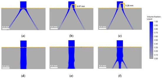
Figure 11.
Instantaneous liquid fraction profile of the spray cone during simulation of the SK nozzle. (a–c) Correspond to µ = 10 mPa·s: (a) pexp = 5 MPa; (b) pexp = 10 MPa; and (c) pexp = 20 MPa. (d–f) Correspond to µ = 35 mPa·s: (d) pexp = 5 MPa; (e) pexp = 10 MPa; and (f) pexp = 20 MPa. For more information about operating conditions, refer to Table 3.
In fact, from what is discussed in the literature, the formation of the air core is heavily influenced by the geometrical dimensions and aspect ratios of the nozzle, especially the outlet channel. In the case of the SK nozzle, the geometry used in this study has a significantly smaller diameter (0.34 mm) than what is usually found in studies where a complete air core could be observed (~1 mm) [32,33]. Even in the case of Maly et al. [12], who had a similar outlet diameter, the length-to-diameter ratio of the outlet channel (~0.5) was significantly lower than the aspect ratio in the nozzle used in our study (~3).
It should be noted that the profiles shown in the figure remained stable with time, so the lack of a spray cone should not be associated with insufficient computing time. Moreover, if one looks at the jet profiles (Figure 11d–f), it is also evident that the turbulence in the liquid jet increases with operating pressure. In fact, at 20 MPa, the jet already begins to break apart within the 1.2 mm length of the simulated airbox. Looking more specifically at the simulated spray profiles with 35 mPa·s in Figure 11, they seem to suggest that the liquid exits the nozzle as a short jet that breaks up into a twisting thin lamella, which quickly forms the spray cone. The length of this jet would decrease with pressure, which is why its breakup could already be observed for 20 MPa. To provide a better perspective, 3D reconstructions of the spray profiles with 35 mPa·s are shown in Figure A1.
With that line of reasoning, the lack of a spray cone in the simulations would simply be a result of the limited volume of the airbox that is simulated at the nozzle exit. It is also important to remark that the simulated airbox is small compared to the casings of the real nozzles (see Figure 1 and Figure 2). These casings obscure the first 3–5 mm after the nozzle exit, so a jet shorter than that would not be observable in the experimental setup. To prove this hypothesis, an additional simulation was performed, at pexp = 20 MPa, with an airbox that had three times the length of the one used for the profiles shown in Figure 11. As the disintegration of the jet is difficult to visualize on a 2D plane, the jet was reconstructed in 3D. This is shown in Figure 12. With this 3D profile, it is even more evident that, with the simulated flow conditions, the liquid jet breaks up into a thinner lamella and forms the spray cone. Nonetheless, for the calculation of the oil droplet breakup parameters, simulating the complete formation of the spray cone was not necessary. Thus, no further simulations were carried out with the larger airbox. With respect to the oil droplet breakup, the lack of a cylindrical air core contradicts the first assumption (see Section 1) for the shear-rate estimations from Taboada et al. [9], although a stable spray cone can still form, as was seen in both the simulations and in the experiments.
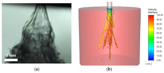
Figure 12.
Spray cone formed during atomization with the SK nozzle for 35 mPa·s at pexp = 20 MPa: (a) Experimental 2D profile; and (b) 3D reconstruction of the simulated spray cone with a 3.3 mm high airbox. The red cylinder is the airbox.
5.2.2. Spray Angle Evaluation
In the experiments, the spray angle was measured for both viscosities and all three pressures, but it could only be measured in the simulations in the cases where a spray cone fully developed. Table 3 shows all these spray angles for the SK nozzle. Because there is a difference between the experimental (pexp) and the simulated (psim) pressures, both are indicated in the table. Looking at the spray angles from the simulations, there is a sharp decrease between 5 and 10 MPa, which is probably related to the appearance of the air core. As the pressure increases further to 20 MPa, and the air core grows, the spray angle continues to decrease slightly. However, the amount of decrease is definitively smaller once the partial air core is already formed, in comparison to when it appears between 5 and 10 MPa.
Table 3.
Simulated (sim) and experimental (exp) spray angles θ, as well as the simulated axial (uax) and rotational (urot) velocities, for different viscosities at the outlet of the SK nozzle under different pressures. The swirl number (S), which is the ratio between the two velocities, is also indicated.
The experimentally measured angles do not follow the same trend. In the experiments, the spray angle has the lowest value at 5 MPa. As the pressure increases, the spray angle has a sharp increase to 56° and then remains relatively constant. In this stage, the experimental and simulated spray angle are approximately the same. With respect to the viscosity of 35 mPa·s, the measured spray angles are consistently smaller than the ones with a lower viscosity. The values do not show a clear tendency, though the largest angle is found at the highest pressure.
It is not completely clear why there is a large deviation between the experiments and simulations for 10 mPa·s at 5 MPa. The spray angles match quite well for the other two pressures. The most plausible cause is that there are phenomena that occur in the real system that are not considered in the simulation. A likely candidate is the effect of surface tension. This becomes noticeable when comparing the spray profiles at 5 and 10 MPa, which are shown in Figure 13. The main difference is that at 5 MPa, the lamella remains continuous for a large part of the recorded spray cone. In comparison, the spray cone at 10 MPa is mostly broken up into droplets by the time it leaves the nozzle casing and enters the recording area. It may be that the continuous lamella presents surface tension effects that lead to a smaller spray angle and that are not accurately represented in the simulation. Although the VOF model does account for surface tension using the Continuum Surface Tension method [34], it was not designed to model surface-tension-driven flows such as the continuous annular liquid sheet seen in Figure 13a. When the lamella quickly breaks apart, the shape of the spray cone is driven by the velocity of the liquid phase and of the resulting droplets, which can be calculated accurately with VOF.
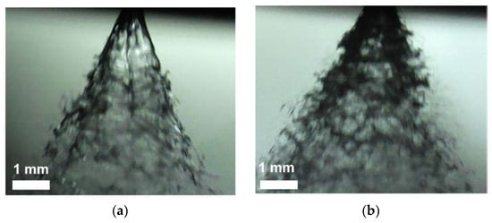
Figure 13.
Experimental profile of the spray cone formed with the SK nozzle for 10 mPa·s at: (a) pexp = 5 MPa and (b) pexp = 10 MPa.
5.2.3. Validation of Simulated Flow Conditions
To understand how the flow inside the atomizer affects the resulting spray profile and the formation, or lack thereof, of the air core, we analyzed the flow condition in the nozzle. One way to do so is through dimensionless numbers such as the Reynolds number—Re—(ratio between axial momentum and viscous forces), Froude number—Fr—(ratio between the rotational momentum and gravitational forces), and swirl number—S—(ratio between axial and rotational velocities), similar to nondimensional analyses performed for vortex formation in stirring tanks [12,35]. With this perspective in mind, the studies that present complete cylindrical air cores do so at much lower Fr or much higher Re. Maly [12] reported Fr < 500. In comparison, the values in our simulated cases were around 1300 when using the same definition of Fr that Maly used. On the other hand, Lee et al. [32] only reported complete air cores for Re > 3300, while, as mentioned in Section 4.2, the Re in our case did not surpass 2200. The swirl number provides further explanation about the behavior of the spray angle. In general, a larger S, and correspondingly a larger axial velocity, should lead to a smaller spray angle. Therefore, we calculated the axial and rotational velocities, and the corresponding swirl number, at the nozzle outlet for the different viscosities and operating conditions, which are also shown in Table 3.
In the case of 10 mPa·s, the swirl number increases, and the spray angle should decrease. Following from what was discussed for the spray cone formation (Figure 11), the increase of S should be a direct consequence of the existence and growth of an internal air core. As pressure, and consequently volume flow, increases, both axial and rotational velocities increase. When there is an internal air core present, the larger rotational velocity causes it to grow, reducing the available cross-sectional area for the liquid to flow through. This further accelerates the liquid axially, causing the increase of S. In comparison, for 35 mPa·s, where there is no air core, the swirl number decreases with pressure, because there is no compounded double effect on the axial velocity. As a result, the spray angle should increase slightly with the pressure. While this could not be directly seen from the experiments, the largest spray angle was indeed observed at the highest pressure. This general behavior was also reported by Lee et al. [32]. They concluded that there were different regimes that dictated how the spray angle changes with pressure. When there is no visible air core inside the nozzle, the spray angle increases with pressure. When there is a partial air core that grows with pressure, the spray angle decreases with pressure.
In conclusion, the analysis of the swirl number and the velocities seen in the simulation match the behavior that would be expected from the literature. They also match the spray angles and the behavior of the air core, or its absence, in the simulations. This means that the velocity profile is internally consistent with the simulated liquid profiles observed. Additionally, it is shown that the simulation recreates the formation of the spray cones that are seen in the experiments, even if, for 35 mPa∙s, this happens outside of the simulated airbox. For 10 mPa∙s, where the spray angles could be specified from the simulation, the values match the experimental ones well for 10 and 20 MPa. The difference observed for 5 MPa may be related to the constricting effects of surface tension on the continuous lamella of the spray cone, which is not properly modelled in the simulations. Even with the recognized limitations, the CFD model seems to consistently recreate the flow conditions inside of the nozzle, which means its predictions concerning the breakup parameters should be reliable.
5.3. Validation of Predicted Flow Behaviour for the MiniSDX Nozzle
5.3.1. Spray Cone Formation
Figure 14 shows snapshots of the liquid profile for the MiniSDX nozzle for the viscosities 10 and 35 mPa·s, at different pressures. The sections shown are the outlet channel of the nozzle and the airbox. The nozzle exit is marked with a dotted orange line. In the case of the MiniSDX, no proper air core can be seen to entrain into the nozzle. Instead, the liquid forms a short jet at the outlet of the swirl chamber for all simulated pressures and viscosities. This stands in contrast to the observations from the SK nozzle, where a liquid jet was only observed for 35 mPa·s. The main reason for this difference between the nozzles is believed to be that the outlet channel of the MiniSDX is conical, while the outlet channel of the SK is cylindrical. Consequently, in the MiniSDX, there is no wall-bounded channel where the flow and the air core can develop. The cases found in the literature, such as the study by Renze, Heinen, and Schönherr [10], who reported air core buildup inside of the chamber, used an SDX-type nozzle with a much larger outlet diameter of 2.3 mm. This is almost six times larger than the outlet of the nozzle used in this study.
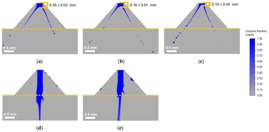
Figure 14.
Instantaneous liquid fraction profile of the spray cone during simulation of the MiniSDX nozzle. (a–c) Correspond to µ = 10 mPa·s: (a) pexp = 5 MPa; (b) pexp = 10 MPa; and (c) pexp = 20 MPa. (d,e) Correspond to µ = 35 mPa·s: (d) pexp = 5 MPa and (e) pexp = 10 MPa. Operating conditions are shown in Table 4.
Although a liquid jet could be observed in all cases for the MiniSDX, the spray formation was different for the two viscosities. In the case of 10 mPa·s, the jet quickly develops into a spray cone within the simulated region (airbox). For each pressure, the length of the jet from the exit of the swirl chamber to the beginning of the spray cone is indicated in Figure 14a–c. Although the liquid that exits the nozzle stably forms the jet and the spray cone, both tend to oscillate unsteadily from side to side, changing slightly in size. To account for this unsteadiness, the jet length was measured in the ten instantaneous liquid profiles, which were also used to measure the spray angle. The average of the measurements, along with the standard deviation, is presented in Figure 14. From this analysis, it is evident that the liquid jet becomes shorter as the pressure increases. On the other hand, for 35 mPa·s, no fully developed spray cone can be observed in the airbox. Nonetheless, the jet stills breaks up into a thinner lamella, and the jet length decreases when the pexp rises from 5 to 10 MPa. To provide a clearer perspective, a 3D reconstruction of the liquid profile is shown in Figure A2 for 35 mPa·s.
5.3.2. Spray Angle Evaluation
Similar to the SK nozzle, the spray angle was only calculated for the simulations with 10 mPa·s, while it was experimentally determined for both viscosities and all three pressures. Table 4 shows the spray angles for the MiniSDX nozzle. For 10 mPa·s, the simulations and experiments show a similar trend: higher pressures tend to lead to narrower angles. There is also a good match between the angles from the simulations and experiments. In the case of 35 mPa·s, a much narrower experimental spray angle is observed at 5 MPa than at 10 MPa. This stands in contrast to the expected behavior, in that the angle should decrease with pressure. A possible explanation for this becomes evident when comparing the spray cones at 5 MPa for both viscosities, as shown in Figure 15. At the lower viscosity, the lamella of the spray cone breaks apart into droplets directly after leaving the nozzle. At the higher viscosity, the lamella remains continuous for a large part of the recorded spray cone. This can cause surface tension effects that keep the spray cone from expanding, reducing the spray angle. Similar effects were also discussed for the SK nozzle (see Figure 13). When the pressure increases to 10 MPa, the lamella breaks again directly after the nozzle outlet (see Figure 15c), so the value of the spray angle returns to the range observed for 10 mPa·s.
Table 4.
Simulated (sim) and experimental (exp) spray angles θ, as well as the simulated axial (uax) and rotational (urot) velocities, for different viscosities at the outlet of the MiniSDX nozzle under different pressures. The swirl number (S), which is the ratio between the two velocities, is also indicated.
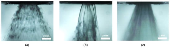
Figure 15.
Experimental profile of the spray cone formed during atomization with the MiniSDX nozzle: (a) µ = 10 mPa·s and pexp = 5 MPa; (b) µ = 35 mPa·s and pexp = 5 MPa; and (c) µ = 35 mPa·s and pexp = 10 MPa.
5.3.3. Validation of Simulated Flow Conditions
To correlate the flow conditions with the observed spray angles, we calculated the velocities and the swirl number for the MiniSDX, which are shown in Table 4. It is important to keep in mind that, for the MiniSDX, the liquid lamella does not form inside the confined regions of a cylindrical outlet channel as with the SK nozzle. Instead, the liquid exits the MiniSDX still as a short-lived jet, and the formation of the air core occurs without the limitations of a channel. However, when the liquid jet remains short, as in the case of 10 mPa·s, the relation between the swirl number and spray angle remains the same as with the SK nozzle: When pressure increases, the swirl number increases and the spray angle decreases (see Table 4). The same behavior would be expected with higher pressures, since the air core would begin to entrain and grow in size inside of the swirl chamber. For the case of 35 mPa·s, the liquid jet is significantly longer (see Figure 14). In that case, the swirl number decreases with pressure, and the spray angle consequently increases. This is the same behavior as seen with the SK nozzle (see Table 3).
The difference between the mechanisms of spray cone formation in the geometrically different nozzles needs to be emphasized. Due to the cylindrical outlet of the SK nozzle, the kinetic energy of the liquid is already distributed in the final axial and rotational velocities, which will define the spray cone angle, in the moment it exits the nozzle. This was the assumption of Taboada et al. [4] when defining the spray angle. On the other hand, the liquid exits the MiniSDX as a short-lived jet, and the formation of the air core occurs without the limitations of a channel. This means that the kinetic energy can also distribute into radial momentum, which is not contemplated by the swirl number. This effect could not be contemplated by the model of Taboada et al. [4].
To summarize, the internal consistency between simulated velocities, spray cone profiles, and spray angles shows again a high reliability of the simulation. The limitations of the simulation concerning the effects of surface tension should not affect the calculation of breakup parameters, which is the main focus of this study. Additionally, the experimental spray angles show a good agreement with the simulated spray angles that could be measured.
5.4. Determination of Oil Droplet Breakup Parameters
With the process and flow conditions already validated, the model was used to predict the breakup parameters, i.e., the deformation stresses and deformation time, for the oil droplets inside of the atomization nozzles. To know which sections of the nozzles we should focus on, we first identified the regions where the highest shear rates occur. These regions of interest are shown in Figure 16. Following what we expected, the outlet channels of both nozzles present high shear rates. Additionally, high-shear regions can be observed at the top of the swirl chambers. These are probably caused by the rotation axis of the swirl flow. Finally, the inlet ports also appear to be regions of interest.
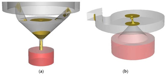
Figure 16.
Simulation with 10 mPa·s liquid in (a) SK nozzle at pexp = 10 MPa and (b) MiniSDX nozzle at pexp = 10 MPa. Yellow areas are regions with shear rates above 106 s−1.
5.4.1. Deformation Stresses
Using the procedure described in Section 4.5, we calculated the instantaneous shear stress and accumulated shear stress history (SSH) profiles, with the two different liquid viscosities, two nozzles, and three pressures. Because of the large number of resulting profiles, these are shown in Appendixe B and Appendixe D. Some general remarks about the profiles are included there. Nonetheless, in short, regardless of the nozzle type, viscosity, and pressure, all profiles clearly show two peak stresses: one in the inlet ports and one in the outlet channel. These two maximum instantaneous stresses are shown in Table 5. To account for the combined effect of deformation stress and time, the amount of increase in the SSH is also shown for both nozzle sections.
Table 5.
Maximum instantaneous shear stress (τmax) and increase of the accumulated shear stress history (ΔSSH) in the inlet ports and outlet channel for different pressures, viscosities, and nozzle types.
The most evident observation is that, for all cases, the highest shear stress is found at the nozzle outlet. At first glance, this coincides with the second assumption stated by Taboada et al. [9]: Oil droplets experience the highest shear rate at the outlet channel. It is interesting to see that this remains true even for 35 mPa·s, when there is no air core present inside of the nozzle. The values also seem to be fairly similar between the two nozzles. In contrast, the simulated peak shear stresses in the inlet port section are consistently smaller for the MiniSDX than for the SK nozzle. This is probably related to the fact that the inlet port of the MiniSDX is wider and has a spiral shape.
However, the increase in the SSH tends to be larger in the inlet ports than in the outlet channel. The only exception is seen for the SK nozzle, with 10 mPa∙s and 20 MPa. As will be seen in Section 5.4.2, the main reason for the larger jump in SSH is that the residence time of the droplets is much larger in the inlet ports compared to the outlet channel. Consequently, while the shear stresses at the inlet port might not be as high as the ones at the nozzle outlet, they are applied for significantly longer periods. This supports the idea that the inlet ports are also an important section for the droplet breakup.
With respect to viscosity, a larger value causes higher shear stresses, which was expected. In most cases, this increase seems to be proportionally similar for the inlet ports and the outlet channel. There is an exception for the SK nozzle, more particularly, at pressures that presented a partial air core for 10 mPa·s and no air core for 35 mPa·s: 10 and 20 MPa. At these pressures, raising the viscosity by 350% caused a 500% increase of the inlet shear stresses but only a 150% increase of the outlet shear stress. The disappearance of the air core with the increased viscosity is believed to be the main cause. While a higher viscosity has a direct positive effect on the shear rate, the resulting lack of an air core means the liquid has more available cross-sectional area to flow out of the nozzle. This has an opposite effect on the shear rate. In comparison, the inlet shear stresses only experience the positive effect of the viscosity.
On the subject of the effect of operating pressures on the deformation stresses, it is fairly noticeable that the peak shear stress at the outlet channel increases sharply with operating pressure (and therefore with volumetric flow). In comparison, the peak shear stress at the inlet ports does not change in a consistent manner. One would expect that the stresses should always increase with a higher volume flow. It may be that an analysis with a larger number of particles would provide more information. It might also reduce the standard deviation in the calculated values. However, such an analysis would have to be carried out with an automated algorithm that can process more particles, since the post-processing of the particles is fairly time-consuming (see Section 4.5); thus, it was not feasible to include in this study. The fact that the outlet shear stresses behave as expected also indicate that it is unlikely to be an artifact or error of the simulation. At any rate, the fluctuating behavior of the inlet ports explain why there is the exceptional case for the SSH with the SK nozzle at 20 MPa. While the outlet stresses increase consistently with pressure, the inlet stresses tend to decrease in this case.
Additional to the shear stresses, breakup can also occur because of elongation of the oil droplets. Therefore, it is important to have information about the elongation stresses along the chosen path lines. The resulting profiles are shown for the SK nozzle in Appendix C and the MiniSDX in Appendix E. Following an analysis similar to the one for the shear stresses, we calculated the maximum elongation stresses in the inlet ports and the outlet channel. The results are summarized in Table 6. However, it is important to remark that the simulated elongation stresses appear to happen in short instantaneous bursts followed by relaxation periods. None of these instantaneous stresses lasts longer than 0.1 µs. We do not believe that this behavior is a physically correct representation of the actual stresses that the droplets experience. The noncontinuous profile might be caused by the numerical error of both the integration method of the streamlines (see Section 4.5) and the first-order discretization scheme used to calculate the derivative in Equation (3). Moreover, the calculated acceleration values, and with them, also the determined stresses, might be overestimated by the simulations, since the tracked particles are massless, which means that they have no inertia and instantly have the same velocity as the surrounding liquid at any point. This could be further improved in a future study by running transient simulations with particles that have the actual density and expected sizes of the oil droplets. This type of simulation would take, however, significantly more time than the steady streamlines calculated in this study.
Table 6.
Maximum (δmax) and average (δavg) instantaneous elongation stress in the inlet ports and outlet channel for different pressures, viscosities, and nozzle types.
It is very likely, then, that the actual peak stresses are lower than the maximum values from the simulation. As a first approximation, we averaged the elongation stresses within each of the two nozzle sections. The average was skewed towards the larger values by using only the measured stresses that surpassed 1 kPa. These averaged values are also shown in Table 6. We would expect that the actual peak stress lies somewhere between the maximum and the averaged values. This means that if we identify droplet breakup in our analysis on basis of the averaged values, this finding would still hold true for the actual stresses.
In general, the elongation stresses follow a similar trend to the shear stresses. They reach larger values in the outlet channel than in the inlet port(s), and they increase with viscosity. However, they do not show a consistent increase with pressure, not even in the outlet channel. Comparing them to the shear stresses, one can notice that the two stresses lie in a similar order of magnitude, especially in the inlet ports, even though the elongation stresses are averaged, while the shear stresses are calculated from the maximum value. In fact, for the MiniSDX nozzle with 10 mPa·s, the elongation stresses are larger than the shear stresses. This does not necessarily agree with previous estimations, where the elongations stresses are assumed to be at least one order of magnitude smaller than the shear stresses [10]. For the outlet channel, the shear stresses are consistently at least an order of magnitude larger than the elongation stresses, except for the MiniSDX with 35 mPa∙s. Although there is still the caveat that the actual peak elongation stresses may be larger, the fact that the shear stresses are, on average, 500% larger than the averaged elongation stresses indicates that they will also most probably be larger than the actual ones.
5.4.2. Deformation Time
As mentioned in Section 4.5, not only are the deformation stresses important to model droplet breakup but also the deformation time. Because residence time is more of a distribution than a single value, the characteristic percentiles t10,0, t50,0, and t90,0 were calculated. For the SK nozzle, the calculated values are presented in Table 7 for the different viscosities and pressures. For the outlet channel, only the median is given because all three percentiles shared similar values. This is probably due to the narrow and cylindrical shape of the outlet channel. The droplets tend to follow similar spiraling paths along the channel and quickly exit the nozzle, so they have similar residence times. As expected, droplets in the swirl chamber have the largest and the widest residence time distribution. Droplets in the outlet have the lowest residence time. If one assumes the deformation time of the oil droplets in a given section is equal to the residence time in that section, then the average deformation time in the outlet channel is consistently around 15% of the one in the inlet ports. With respect to the process conditions, the residence time in all sections decreases with higher operating pressures and viscosities, since both are correlated with higher volume flows.
Table 7.
Residence time through the different sections of the SK nozzle: the inlet port, the swirl chamber, and the outlet channel.
The calculated residence times in the MiniSDX nozzle are presented in Table 8. In general, they follow the behavior seen for the SK nozzle. The average deformation time in the outlet channel is between 12 and 20% of the average deformation time in the inlet ports. However, a couple of differences can be mentioned. First, the overall residence time in the MiniSDX nozzle is longer than in the SK nozzle. Second, the inlet port presents consistently larger residence times than the swirl chamber. Since the inlet port of this nozzle is wider and larger than that of the SK nozzle, this was expected.
Table 8.
Residence time through the different sections of the MiniSDX nozzle: the inlet port, the swirl chamber, and the outlet channel.
6. Evaluation of Droplet Breakup
6.1. Emulsion Theory
Looking at the stress histories from Table 5, along with the deformation times from Section 5.4.2, it seems that both the inlet ports and the outlet channel might play a role in the droplet breakup. This is seen for the SK nozzle as well as for the MiniSDX. While the peak shear stresses at the inlet are about one order of magnitude smaller than the peak shear stresses at the outlet, the residence time at the inlet ports is consistently 5–8 times longer than in the outlet channels. To evaluate the significance of the two sections of interest with respect to droplet breakup, we performed an analysis based on emulsification theory.
According to this theory, two conditions must be fulfilled for droplet breakup to occur [36] (pp. 142–149). On the one hand, the ratio between the local deformation stresses on the droplet and its own capillary pressure ( must exceed a critical value. This ratio is characterized by the capillary number () [37]. In a laminar flow, can be defined for shear and/or elongation stresses as follows:
where refers to the dynamic viscosity of the continuous phase, which is the same as the emulsion viscosity. For a spherical droplet, the capillary pressure can be derived from the Laplace equation, as follows [38]:
where is the droplet diameter, and is the interfacial tension between the two liquid phases. The critical capillary number () that must be exceeded for droplet breakup was described by Grace [27]. The author showed that depends on the viscosity ratio between the disperse and continuous phases and on the kinds of stress that are applied. For a given deformation stress, the can be used along with the appropriate part of Equation (4) and with Equation (5) to determine the maximum droplet size that can no longer be broken apart (xmax).
On the other hand, the deformation time () must exceed a critical value as well. For a laminar flow, this critical value can be estimated using the equation from Walstra and Smulders [39]:
where refers to the dynamic viscosity of the disperse phase; and are calculated from Equations (1) and (2), respectively. Similar to the capillary number, the critical deformation time depends on the deformation stress and the capillary pressure. The latter, in turn, depends on the droplet size. However, for the critical time calculation, the droplet size does not refer to the maximum resulting droplet size, but rather to the initial droplet size that is subjected to the deformation stress. With decreasing droplet sizes, increases to infinity.
6.2. Two-Step Droplet Breakup Inside of the Nozzles
From the simulation results, we know that there are two regions of interest for the droplet breakup: the inlet ports and the outlet channel. With that in mind, we decided to evaluate the droplet breakup as a two-step process: an initial breakup in the inlet ports followed by a secondary breakup in the outlet channel. For critical time calculations, the 90% volumetric percentile (x90,3) of the initial oil droplet size distribution of the feed emulsion (44 μm) was used. σ was taken from Taboada et al. [9] as 11.8 mN/m for the emulsion of 10 mPa∙s, and 12.6 mN/m for 35 mPa∙s. The dynamic viscosity of the disperse phase (MCT-oil) is 29 mPa∙s [4]. Due to the viscosity ratios, the shear is 0.66 for 10 mPa·s and 0.55 for 35 mPa·s [27]. For elongation stresses, is 0.12 for 10 mPa·s and 0.15 for 35 mPa·s.
6.2.1. Breakup at the Inlet Ports
First, the xmax that would result based on the simulated stresses, as well as their required critical deformation time, were first calculated for the inlet ports of both nozzles. The results of the analysis are summarized in Table 9. In effect, the results show that, for all cases, both shear and elongation stresses are high enough to lead to a droplet breakup. Also, the median residence times t50,0 (see Table 7 and Table 8) are always one to two orders of magnitude larger than the critical deformation times. The smallest xmax from both types of stresses was chosen as the theoretical intermediary droplet size xmax,ip that would go from the inlet ports through the swirl chamber into the outlet channels. For most cases, the intermediate sizes were defined by the elongation stresses, with only one exception for the SK nozzle with 35 mPa·s. The effect of the elongation stresses is particularly clear for the MiniSDX nozzle, where the shear stresses alone would lead to droplet sizes over five times larger than the ones caused by the elongation stresses. The contraction from the wide inlet regions to the comparatively narrow inlet ports (see internal volumes in Section 4.1) may be the cause for this strong effect of the droplet elongation.
Table 9.
Largest theoretical droplet size (xmax) and critical deformation time (tcr) for different pressures, viscosities, and nozzle types for the inlet ports. The shear and elongation stresses are compared, and the theoretical intermediary droplet size inside of the nozzle is shown.
In principle, the fact that droplet breakup occurs in the inlet ports would go against the third assumption used in the model of Taboada et al. [9], according to which, the highest shear rate at the outlet channel should be the single deciding factor for the oil droplet size. However, this does not mean that the droplet size cannot be correlated with the shear stresses at the nozzle outlet. Following Equation (4) and general emulsion theory [36], the capillary number does not depend on the initial size of the oil droplets. This means that as long as the outlet channel also fulfills the breakup criteria, the final droplet size would still be defined by the outlet stresses, regardless of what happened at the inlet ports.
6.2.2. Breakup at the Outlet Channels
To evaluate if this is the case, the same calculation as for the inlet ports was executed for the outlet channels of both nozzles. For the critical deformation times, the droplet size in Equation (6) was set as the intermediary xmax obtained from the inlet ports. The results of this analysis are shown in Table 10. It is interesting to see that the two nozzles present opposite behaviors with respect to the predicted droplet size. In the SK nozzle, the shear stresses lead in most cases to the smallest droplets, but the droplet sizes resulting from the stresses are often in the same range. In the MiniSDX nozzle, the elongation stresses are dominant for the smallest droplets. However, the most evident result is that the equation for the critical deformation time presents negative values for most of the cases analyzed. Following the theory from Section 6.1, this would mean that droplet breakup cannot occur because tcr is infinite. In other cases, the values exceed the residence time inside of the nozzle, leading to the same conclusion. There are a few exceptions. Some correspond to the cases where there was an internal air core and, consequently, a liquid lamella: the SK nozzle with 10 mPa·s at 10 and 20 MPa. The acceleration of the liquid as it passes through the thin lamella is most likely what causes the shear stress to be high enough to surpass the predicted capillary pressure. The other cases happen with the MiniSDX nozzle with 35 mPa·s. They may be related to the low deformation stresses in the MiniSDX in comparison to the SK nozzle, because of the wider and curved inlet port.
Table 10.
Largest theoretical droplet size (xmax) and critical deformation time (tcr) for different pressures, viscosities, and nozzle types for the outlet channel. The adjusted critical deformation time (tadj,cr) is also calculated. The shear and elongation stresses are compared, and the final droplet size is shown. The experimental values shown are taken from Taboada et al. [9].
From the previous results, it might seem that the outlet channel does not cause further breakup of the droplets. However, some caveats must be addressed when discussing this analysis. The fact that both shear and elongation fulfill the breakup criteria at the inlet ports indicates that the breakup mechanism of the droplets involves both forces. In fact, such type of deformation, in which the droplet stretches in one direction before the ligament breaks up from the elongation or from shearing, was already described by Feigl et al. [40]. Their system had a similar viscosity ratio (~0.6) but lower deformation rates (102–103 s−1). Nonetheless, if the mechanism can occur at those lower shear and elongation rates, it most likely also takes place inside the nozzle that we analyzed. A more realistic model would require a more complicated emulsification mechanism than the one explained in Equations (4)–(6). Not only is the system not really in an equilibrium state, like the theoretical model assumes [36] (pp. 142–149), but the oil droplets have been proven to deform into elongated threads inside of the nozzle, under the same order of magnitude of shear and elongation rates as the ones seen in our study [41].
A more nuanced approach might be to account for the fact that the droplets that reach the outlet channel are not spherical but cylindrical. For the critical deformation time, this would mean adjusting the capillary pressure with a factor of two, instead of four, in Equation (5). There is, unfortunately, no way to adjust the intermediary or final droplet sizes, since the Cacr from Grace [27] was specifically determined for spherical droplets. Nevertheless, the analysis would still give us some information on whether the shear or elongation stresses play a deciding role in the droplet breakup at the nozzle outlet. With these considerations, the critical deformation times were recalculated and are shown in Table 10. The final predicted droplet size that would exit the nozzle from this calculation is also indicated, as xmax,oc. With this adjusted approach, the shear stresses always fulfill the breakup criteria at the outlet channel, while the elongation stresses only do so for the MiniSDX with 35 mPa·s. Even then, they only provide slightly smaller droplet sizes than the ones calculated from the shear stresses. This would indicate that the breakup in the outlet is indeed driven by the shear stresses. At this point, it is important to remember that the discussion of the elongation stresses extracted from the simulation is limited by the uncertainties discussed in Section 5.4.1.
6.3. Correlation with Experimental Droplet Sizes
When relating Equation (4) to experimental droplet size distributions, Taboada et al. [4] utilized the oil x90,3 in lieu of the theoretical xmax,oc that would come out of the nozzle. Following the same logic, the experimental x90,3 from Taboada et al. [9] is also shown in Table 10 for the SK nozzle, which is the geometry that they used in their study. The predicted values follow the same tendency for pressure as the measured ones: smaller diameters at higher pressure. However, the tendencies do not match when looking at the viscosity. While, according to emulsion theory, the end droplet size should always decrease with viscosity, because the deformation stresses are higher, this is not seen in the experiments. It is interesting to note that the predicted values are consistently smaller than the ones measured in the experiment. To be precise, they are around 70% of the experimental value for 10 mPa·s and around 30% of the experimental value for 35 mPa·s. The fact that the predictions seem to have a constant error for a given viscosity and follow the expected behavior with pressure could indicate that the theoretical model might just be using the wrong . If the error originated from the deformation stresses, it would not be constant between pressures, since the stresses are calculated independently for each case.
Following this assumption, we utilized the correlation established by Taboada et al. [9] for the SK nozzle, which linked the experimental x90,3 with the maximum shear rate calculated at the outlet channel of the nozzle. For this, they used the same definition of the shear capillary number as established in Equation (4). However, instead of using the Cacr from Grace [27], Taboada et al. [9] proposed that the critical value depended on the geometry of the nozzle and that the viscosity of the emulsion should be atomized. Based on this, we recalculated the regression fittings of their study using the shear stresses obtained from the simulations to see if they provide a better correlation. The results are shown in Figure 17. Taboada et al. [9] reported a good fit for 10 mPa·s, with an R2 of around 0.94. This good fit is still maintained with the CFD approach, with an R2 of 0.98. The real improvement can be seen for 35 mPa·s, where they reported deviations from the proposed model and a R2 of around 0.87. In comparison, with the CFD predictions of the shear stresses, the R2 increases up to 0.99. The main difference observed is that the inviscid approach proposed by the previous work over-predicted the shear stresses with the higher viscosity. This is mostly due to the assumption that there would be an air core present under those conditions, which is not the case.
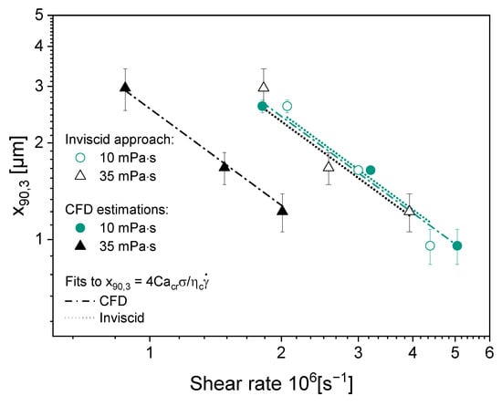
Figure 17.
Values of x90,3 of oil droplet size after atomization with the SK nozzle, for two evaluated viscosities, correlated with the estimated shear rate with the inviscid approach (from Taboada et al. [9]) and with the shear rates determined from the CFD model.
The improved fitting highlights that the numerical model allows us to make more accurate predictions about the system, even when it is used along with simplified theoretical models, such those using the capillary number. Additionally, the simulation allows a more informed decision about which deformation stresses should be used when trying to make predictions about the oil droplet sizes, as it permits the full analysis of a two-step breakup mechanism. Finally, it should be remarked that the results presented in Table 10 and Figure 17 show that the maximum droplet size can indeed be correlated to the outlet shear stresses, even if not all of the assumptions of Taboada et al. [9] could be corroborated. With the corrected correlations, the predicted critical capillary numbers would be 0.96 for 10 mPa·s and 1.78 for 35 mPa·s for the SK nozzle. These are noticeably larger than the theoretical values of 0.66 for 10 mPa·s and 0.55 for 35 mPa·s [27].
7. Conclusions
A numerical model was implemented in ANSYS Fluent software to simulate the multiphase flow in two different types of pressure swirl atomizers: an SK and a MiniSDX nozzle. The main objective was to determine the oil droplet breakup parameters for emulsion atomization, namely the deformation stresses and times. Additionally, we wanted to validate the assumptions that are usually used to theoretically estimate these parameters:
- A complete air core forms inside of the nozzles.
- The highest shear rate is found at the nozzle outlet channel.
- This shear stress at the nozzle outlet is correlated with the final oil droplet size.
The CFD model assumed that the air and the liquid were Newtonian and incompressible, and the flow regime was assumed to be laminar. The mesh density was selected to minimize the discretization error without incurring unnecessary computational costs. With this model, the process conditions during the atomization of two emulsions of different viscosities (10 and 35 mPa·s) were recreated. This was compared with experimental data to validate the numerical model. An average error of around 15% was concluded to be acceptable, since the fixed mass flow inlet should ensure that the velocity gradients and shear rate calculations remain accurate.
With the implemented model, the flow distribution and the formation of the spray cone were analyzed in both types of nozzles for different geometries and pressures. With this analysis, we found that no complete cylindrical air core formed inside of the nozzles. This is most likely related to the relatively small outlet diameters of the nozzles used in this study and, in the case of the SK nozzle, to the large length/diameter ratio of the outlet channel. A partial air core still forms in the SK nozzle for the emulsion of 10 mPa·s. In all other cases, including the MiniSDX, a short liquid jet exits the nozzle before it breaks up into a twisting thin lamella that forms the spray cone. The presence of an air core affects how the spray angle changes with operating pressure. This was evidenced in both experiments and simulations.
Although the complete air core could not be evidenced for these nozzle geometries, the highest shear rate was indeed found at the outlet channel for both nozzles under all conditions. Additionally, a correlation can be made between this shear rate and the maximum droplet size (x90,3), with an R2 of up to 0.99. However, this does not mean that the outlet shear rate is the only defining deformation force on the droplet breakup. Both the shear rate at the inlet ports of the nozzles, and the elongation stresses along the nozzle were proven to fulfill the necessary criteria to cause droplet breakup. The theoretical model, which is based on the capillary number, cannot account for this multi-step, multi-factorial breakup mechanism. A more rigorous and complete model would have to be developed to be able to consider all the different deformation forces on the droplets.
Author Contributions
Conceptualization, M.Á.B.M. and V.G.; methodology, M.Á.B.M. and V.G.; software, M.Á.B.M.; validation, M.Á.B.M.; formal analysis, M.Á.B.M.; investigation, M.Á.B.M.; resources, V.G.; data curation, M.Á.B.M.; writing—original draft preparation, M.Á.B.M.; writing—review and editing, M.Á.B.M. and V.G.; visualization, M.Á.B.M.; supervision, V.G.; project administration, V.G.; funding acquisition, V.G. All authors have read and agreed to the published version of the manuscript.
Funding
This research was carried out in the frame of an Industrial Collective Research (IGF) project (21539N) of the Research Association of the German Food Industry (FEI), supported via the German Federation of Industrial Research Associations (AiF) within the program for promoting the IGF of the German Federal Ministry for Economic Affairs and Climate Action (BMWK), based on a resolution of the German Parliament.
Data Availability Statement
The data presented in this study are available on request from the corresponding author. The data are not publicly available due to the size of the simulation files.
Acknowledgments
The authors would like to recognize the support by the state of Baden-Württemberg through access to the bwHPC. The authors would also like to thank Martha Taboada, Carolina Gómez, and Nicolás Solano for sharing, or helping in the collection of, experimental data. Additionally, the authors would like to thank Nico Leister, for his advice during the emulsion theory discussion.
Conflicts of Interest
The authors declare no conflict of interest. The funders had no role in the design of the study; in the collection, analyses, or interpretation of data; in the writing of the manuscript; or in the decision to publish the results.
Appendix A. Three-Dimensional Liquid Profiles of the Nozzle Outlets
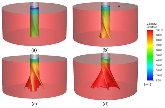
Figure A1.
Three-dimensional profile of the liquid jet formed at the nozzle outlet during atomization of an emulsion of 35 mPa·s, with the SK nozzle at (a) QL = 0.30 L/min (pexp = 5 MPa); (b) QL = 0.44 L/min (pexp = 10 MPa); (c) QL = 0.53 L/min (pexp = 20 MPa); and (d) QL = 0.65 L/min (pexp = 20 MPa, pressure inlet). The red cylinder is the airbox.
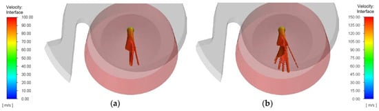
Figure A2.
Three-dimensional profile of the liquid jet formed at the nozzle outlet during atomization of an emulsion of 35 mPa·s, with the MiniSDX nozzle at (a) QL = 0.47 L/min (pexp = 5 MPa) and (b) QL = 0.70 L/min (pexp = 10 MPa). The red cylinder is the airbox.
Appendix B. Shear Stress Profiles for the SK Nozzle
For each profile, the sections of interest in the droplet paths are highlighted in the colored bars. The inlet ports are marked in green; the swirl chamber in grey: and the outlet channel in orange. Some general remarks can be drawn about the profiles. First of all, regardless of the nozzle type, viscosity, and pressure, the randomly chosen particles follow the same trend in their instantaneous stress profile. As the droplets pass through the inlet region, they experience low shear stresses, which then rise to a local maximum peak in the inlet region(s). The stresses lower again, as the droplets cross the swirl chamber, and then finally rise to a global maximum peak somewhere in the outlet channel, before the droplets exit the nozzle. Second, with regard to the accumulated SSH, all profiles show a marked increase as the droplet passes through the inlet port(s). This jump seems to be consistently larger than when it pass through the outlet channel.
The instantaneous and accumulated profiles show that the residence time and the specific stresses each droplet experiences along its path are different. However, the maximum peak values tend to be very similar between the three randomly chosen droplets, especially for the outlet shear stresses. The similarity between the peak values indicates the additional reliability of the stress calculations as well as of the breakup analysis, which will be discussed in Section 6.
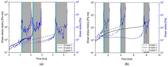
Figure A3.
Accumulated shear stress history (left black axis) and instantaneous shear stress (right blue axis) from three particles along their path throughout the SK nozzle (pexp = 10 MPa) with (a) 10 mPa·s (QL = 0.35 L/min) and (b) 35 mPa·s (QL = 0.44 L/min). For each particle, the path through each of the nozzle sections is highlighted: the inlet ports (green), the swirl chamber (grey), and the outlet channel (orange).
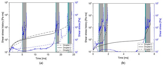
Figure A4.
Accumulated shear stress history (left black axis) and instantaneous shear stress (right blue axis) from three particles along their path throughout the SK nozzle with 10 mPa·s at (a) QL = 0.26 L/min (pexp = 5 MPa) and (b) QL = 0.44 L/min (pexp = 20 MPa). For each particle, the path through each of the nozzle sections is highlighted: the inlet ports (green), the swirl chamber (grey), and the outlet channel (orange).
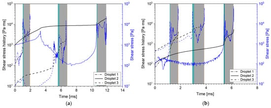
Figure A5.
Accumulated shear stress history (left black axis) and instantaneous shear stress (right blue axis) from three particles along their path throughout the SK nozzle with 35 mPa·s at (a) QL = 0.30 L/min (pexp = 5 MPa) and (b) QL = 0.53 L/min (pexp = 20 MPa). For each particle, the path through each of the nozzle sections is highlighted: the inlet ports (green), the swirl chamber (grey), and the outlet channel (orange).
Appendix C. Elongation Stress Profiles for the SK Nozzle
For each profile, the sections of interest in the particle paths are highlighted in the colored bars. The inlet ports are marked in green, the swirl chamber in grey, and the outlet channel in orange. In the case of the MiniSDX, the travel path of the particles through the inlet region, before they reach the inlet port, was omitted, because it was too long in comparison to the actual travel through the regions of interest, which made visualization difficult.
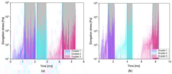
Figure A6.
Instantaneous elongation stress from three particles along their path throughout the SK nozzle (pexp = 10 MPa) with (a) 10 mPa·s (QL = 0.35 L/min) and (b) 35 mPa·s (QL = 0.44 L/min). For each particle, the path through each of the nozzle sections is highlighted: the inlet ports (green), the swirl chamber (grey), and the outlet channel (orange).
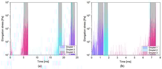
Figure A7.
Instantaneous elongation stress from three particles along their path throughout the SK nozzle with 10 mPa·s at (a) QL = 0.26 L/min (pexp = 5 MPa) and (b) QL = 0.44 L/min (pexp = 20 MPa). For each particle, the path through each of the nozzle sections is highlighted: the inlet ports (green), the swirl chamber (grey), and the outlet channel (orange).
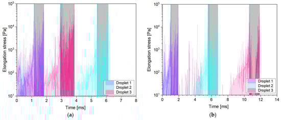
Figure A8.
Instantaneous elongation stress from three particles along their path throughout the SK nozzle with 35 mPa·s at (a) QL = 0.30 L/min (pexp = 5 MPa) and (b) QL = 0.53 L/min (pexp = 20 MPa). For each particle, the path through each of the nozzle sections is highlighted: the inlet ports (green), the swirl chamber (grey), and the outlet channel (orange).
Appendix D. Shear Stress Profiles for the MiniSDX Nozzle
For each profile, the sections of interest in the particle paths are highlighted in the colored bars. The inlet ports are marked in green, the swirl chamber in grey, and the outlet channel in orange. In the case of the MiniSDX, the travel path of the particles through the inlet region, before they reach the inlet port, was omitted, because it was too long in comparison to the actual travel through the regions of interest, which made visualization difficult.
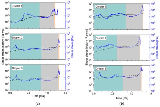
Figure A9.
Accumulated shear stress history (left black axis) and instantaneous shear stress (right blue axis) from three particles along their path throughout the MiniSDX nozzle (pexp = 10 MPa) with (a) 10 mPa·s (QL = 0.53 L/min) and (b) 35 mPa·s (QL = 0.70 L/min). For each particle, the path through each of the nozzle sections is highlighted: the inlet port (green), the swirl chamber (grey), and the outlet channel (orange).
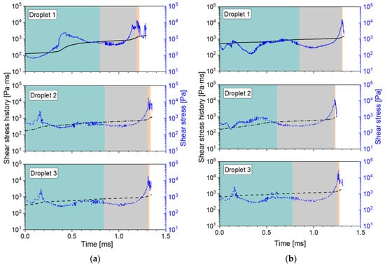
Figure A10.
Accumulated shear stress history (left black axis) and instantaneous shear stress (right blue axis) from three particles along their path throughout the MiniSDX nozzle with 10 mPa·s at (a) QL = 0.40 L/min (pexp = 5 MPa) and (b) QL = 0.66 L/min (pexp = 20 MPa). For each particle, the path through each of the nozzle sections is highlighted: the inlet ports (green), the swirl chamber (grey), and the outlet channel (orange).
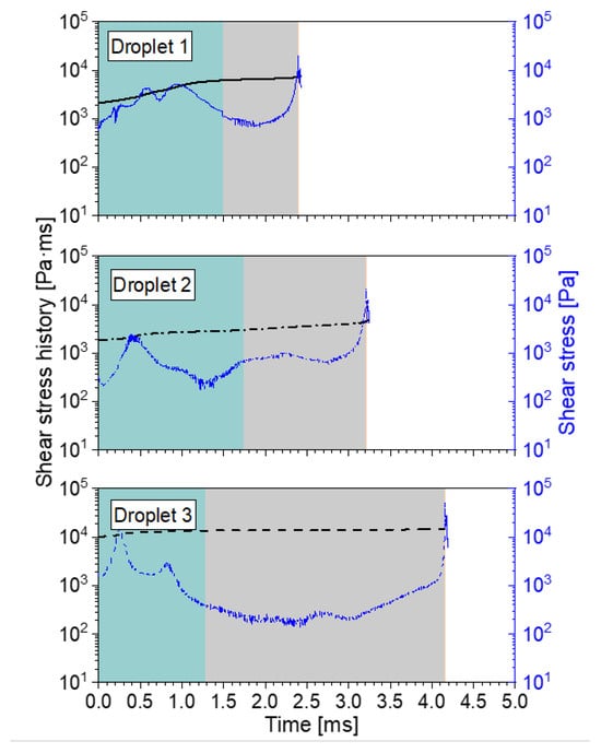
Figure A11.
Accumulated shear stress history (left black axis) and instantaneous shear stress (right blue axis) from three particles along their path throughout the MiniSDX nozzle with 35 mPa·s at QL = 0.47 L/min (pexp = 5 MPa). For each particle, the path through each of the nozzle sections is highlighted: the inlet ports (green), the swirl chamber (grey), and the outlet channel (orange).
Appendix E. Elongational Stress Profiles for the MiniSDX Nozzle
For each profile, the sections of interest in the particle paths are highlighted in the colored bars. The inlet ports are marked in green, the swirl chamber in grey, and the outlet channel in orange. In the case of the MiniSDX, the travel path of the particles through the inlet region, before they reach the inlet port, was omitted, because it was too long in comparison to the actual travel through the regions of interest, which made visualization difficult.
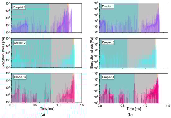
Figure A12.
Instantaneous elongation stress from three particles along their path throughout the MiniSDX nozzle (pexp = 10 MPa) with (a) 10 mPa·s (QL = 0.53 L/min) and (b) 35 mPa·s (QL = 0.70 L/min). For each particle, the path through each of the nozzle sections is highlighted: the inlet ports (green), the swirl chamber (grey), and the outlet channel (orange).
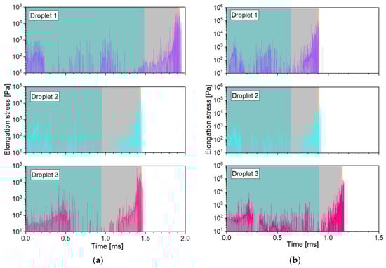
Figure A13.
Instantaneous elongation stress from three particles along their path throughout the MiniSDX nozzle with 10 mPa·s at (a) QL = 0.40 L/min (pexp = 5 MPa) and (b) QL = 0.66 L/min (pexp = 20 MPa). For each particle, the path through each of the nozzle sections is highlighted: the inlet ports (green), the swirl chamber (grey), and the outlet channel (orange).
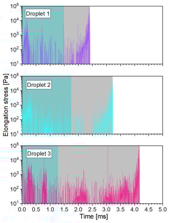
Figure A14.
Instantaneous elongation stress from three particles along their path throughout the MiniSDX with 35 mPa·s at QL = 0.47 L/min (pexp = 5 MPa). For each particle, the path through each of the nozzle sections is highlighted: the inlet ports (green), the swirl chamber (grey), and the outlet channel (orange).
References
- Reineccius, G.A. The Spray Drying of Food Flavors. Dry. Technol. 2004, 22, 1289–1324. [Google Scholar] [CrossRef]
- Vega, C.; Roos, Y.H. Invited review: Spray-dried dairy and dairy-like emulsions--compositional considerations. J. Dairy Sci. 2006, 89, 383–401. [Google Scholar] [CrossRef]
- Del Hernandez Sanchez, M.R.; Cuvelier, M.-E.; Turchiuli, C. Design of liquid emulsions to structure spray dried particles. J. Food Eng. 2015, 167, 99–105. [Google Scholar] [CrossRef]
- Taboada, M.L.; Schäfer, A.-C.; Karbstein, H.P.; Gaukel, V. Oil droplet breakup during pressure swirl atomization of food emulsions: Influence of atomization pressure and initial oil droplet size. J. Food Process Eng. 2021, 44, e13598. [Google Scholar] [CrossRef]
- Barbosa-Cánovas, G.V.; Ortega-Rivas, E.; Juliano, P.; Yan, H. Food Powders: Physical Properties, Processing, and Functionality; Springer: Boston, MA, USA, 2005; pp. 271–304. ISBN 978-0-306-47806-2. [Google Scholar]
- Lefebvre, A.H.; McDonell, V.G. Atomization and Sprays, 2nd ed.; CRC Press: Boca Raton, FL, USA; London, UK; New York, NY, USA, 2017; ISBN 9781498736268. [Google Scholar]
- Walzel, P. Spraying and Atomizing of liquids. In Ullmann’s Encyclopedia of Industrial Chemistry; Wiley-VCH Verlag GmbH & Co. KGaA: Weinheim, Germany, 2000; ISBN 3527306730. [Google Scholar]
- Bolszo, C.D.; Narvaez, A.A.; McDonell, V.; Dunn-Rankin, D.; Sirignano, W.A. Pressure swirl atomization of water-in-oil emulsions. At. Sprays 2010, 20, 1077–1099. [Google Scholar] [CrossRef]
- Taboada, M.L.; Müller, E.; Fiedler, N.; Karbstein, H.P.; Gaukel, V. Oil droplet breakup during pressure swirl atomization of emulsions: Influence of emulsion viscosity and viscosity ratio. J. Food Eng. 2022, 321, 110941. [Google Scholar] [CrossRef]
- Renze, P.; Heinen, K.; Schönherr, M. Experimental and Numerical Investigation of Pressure Swirl Atomizers. Chem. Eng. Technol. 2011, 34, 1191–1198. [Google Scholar] [CrossRef]
- Laurila, E.; Roenby, J.; Maakala, V.; Peltonen, P.; Kahila, H.; Vuorinen, V. Analysis of viscous fluid flow in a pressure-swirl atomizer using large-eddy simulation. Int. J. Multiph. Flow 2019, 113, 371–388. [Google Scholar] [CrossRef]
- Maly, M.; Jedelsky, J.; Slama, J.; Janackova, L.; Sapik, M.; Wigley, G.; Jicha, M. Internal flow and air core dynamics in Simplex and Spill-return pressure-swirl atomizers. Int. J. Heat Mass Transf. 2018, 123, 805–814. [Google Scholar] [CrossRef]
- ANSYS, Inc. Ansys Fluent Theory Guide, Release 2019 R3; ANSYS, Inc.: Canonsburg, PA, USA, 2019. [Google Scholar]
- Maly, M.; Slama, J.; Sapik, M.; Jedelsky, J. 2D and 3D numerical modelling of internal flow of Pressure-swirl atomizer. EPJ Web Conf. 2019, 213, 2055. [Google Scholar] [CrossRef]
- Anderson, J.D. Fundamentals of Aerodynamics, 6th ed.; McGraw-Hill Education: New York, NY, USA, 2017; ISBN 1259129918. [Google Scholar]
- Jabbari, M.; Bulatova, R.; Hattel, J.H.; Bahl, C. An evaluation of interface capturing methods in a VOF based model for multiphase flow of a non-Newtonian ceramic in tape casting. Appl. Math. Model. 2014, 38, 3222–3232. [Google Scholar] [CrossRef]
- Ballesteros Martínez, M.Á.; Gaukel, V. Time-Averaged Analysis and Numerical Modelling of the Behavior of the Multiphase Flow and Liquid Lamella Thickness Inside an Internal-Mixing ACLR Nozzle. Flow Turbul. Combust 2023, 110, 601–628. [Google Scholar] [CrossRef]
- Ballesteros Martínez, M.; Pereyra, E.; Ratkovich, N. CFD study and experimental validation of low liquid-loading flow assurance in oil and gas transport: Studying the effect of fluid properties and operating conditions on flow variables. Heliyon 2020, 6, e05705. [Google Scholar] [CrossRef] [PubMed]
- Zeigarnik, Y.A. Annular flow. In A-to-Z Guide to Thermodynamics, Heat and Mass Transfer, and Fluids Engineering; Begellhouse: Danbury, CT, USA, 2006. [Google Scholar]
- Ramsey, M.S. Rheology, viscosity, and fluid types. In Practical Wellbore Hydraulics and Hole Cleaning; Elsevier: Amsterdam, The Netherlands, 2019; pp. 217–237. ISBN 9780128170885. [Google Scholar]
- Shashi Menon, E. Fluid flow in pipes. In Transmission Pipeline Calculations and Simulations Manual; Elsevier: Amsterdam, The Netherlands, 2015; pp. 149–234. ISBN 9781856178303. [Google Scholar]
- Okumura, K. CFD Simulation by Automatically Generated Tetrahedral and Prismatic Cells for Engine Intake Duct and Coolant Flow in Three Days. In SAE Technical Paper Series; SAE 2000 World Congress, MAR. 06, 2000; SAE International 400 Commonwealth Drive: Warrendale, PA, USA, 2000. [Google Scholar]
- White, F.M. Fluid Mechanics, 8th ed.; McGraw-Hill: New York, NY, USA, 2016; ISBN 978-0073398273. [Google Scholar]
- Schlichting, H.; Gersten, K. Boundary-Layer Theory; Springer: Berlin/Heidelberg, Germany, 2017; ISBN 978-3-662-52917-1. [Google Scholar]
- Petrie, C.J. Extensional viscosity: A critical discussion. J. Non-Newton. Fluid Mech. 2006, 137, 15–23. [Google Scholar] [CrossRef]
- George, H.F.; Qureshi, F. Newton’s law of viscosity, newtonian and non-newtonian fluids. In Encyclopedia of Tribology; Wang, Q.J., Chung, Y.-W., Eds.; Springer: Boston, MA, USA, 2013; pp. 2416–2420. ISBN 978-0-387-92896-8. [Google Scholar]
- Grace, H.P. Dispersion phenomena in high viscosity immiscible fluid systems and application of static mixers as dispersion devices in such systems. Chem. Eng. Commun. 1982, 14, 225–277. [Google Scholar] [CrossRef]
- Spurk, J.H.; Aksel, N. Fluid Mechanics, 2nd ed.; Springer: Berlin/Heidelberg, Germany, 2008; ISBN 9783540735366. [Google Scholar]
- Preiss, F.J.; Rütten, E.; Tröster, A.; Gräf, V.; Karbstein, H.P. Influence of the droplet trajectory on the resulting droplet deformation and droplet size distribution in high-pressure homogenizer orifices. Can. J. Chem. Eng. 2022, 100, 1451–1467. [Google Scholar] [CrossRef]
- Tannehill, J.C.; Anderson, D.A.; Pletcher, R.H. Computational Fluid Mechanics and Heat Transfer, 2nd ed.; Taylor & Francis: Washington, DC, USA, 1997; ISBN 9781560320463. [Google Scholar]
- Galbiati, C.; Tonini, S.; Conti, P.; Cossali, G.E. Numerical Simulations of Internal Flow in an Aircraft Engine Pressure Swirl Atomizer. J. Propuls. Power 2016, 32, 1433–1441. [Google Scholar] [CrossRef]
- Lee, E.J.; Oh, S.Y.; Kim, H.Y.; James, S.C.; Yoon, S.S. Measuring air core characteristics of a pressure-swirl atomizer via a transparent acrylic nozzle at various Reynolds numbers. Exp. Therm. Fluid Sci. 2010, 34, 1475–1483. [Google Scholar] [CrossRef]
- Liu, Z.; Huang, Y.; Sun, L. Studies on air core size in a simplex pressure-swirl atomizer. Int. J. Hydrog. Energy 2017, 42, 18649–18657. [Google Scholar] [CrossRef]
- Brackbill, J.; Kothe, D.; Zemach, C. A continuum method for modeling surface tension. J. Comput. Phys. 1992, 100, 335–354. [Google Scholar] [CrossRef]
- Szeliga, N.; Helmrich von Elgott, L.; Bezecny, D.; Richter, S.; Hoffmann, M.; Schlüter, M. Large-Scale Experiments on the Formation of Surface Vortices with and without Vortex Suppression. Chem. Ing. Tech. 2019, 91, 1802–1811. [Google Scholar] [CrossRef]
- Köhler, K.; Schuchmann, H.P. Emulgiertechnik: Grundlagen, Verfahren und Anwendungen, 3rd ed.; Behr: Hamburg, Germany, 2012; ISBN 978-3-89947-869-3. [Google Scholar]
- Taylor, G. The formation of emulsions in definable fields of flow. Proc. R. Soc. Lond. A 1934, 146, 501–523. [Google Scholar] [CrossRef]
- Jiao, J.; Burgess, D.J. Multiple emulsion stability: Pressure balance and interfacial film strength. In Multiple Emulsions; Aserin, A., Ed.; John Wiley & Sons, Inc: Hoboken, NJ, USA, 2007; pp. 1–27. ISBN 9780470209264. [Google Scholar]
- Walstra, P.; Smulders, P.E. Emulsion formation. In Modern Aspects of Emulsion Science; Binks, B.P., Ed.; The Royal Society of Chemistry: London, UK, 1998; pp. 56–99. ISBN 978-0-85404-439-9. [Google Scholar]
- Feigl, K.; Baniabedalruhman, A.; Tanner, F.X.; Windhab, E.J. Numerical simulations of the breakup of emulsion droplets inside a spraying nozzle. Phys. Fluids 2016, 28, 123103. [Google Scholar] [CrossRef]
- Qin, K.; Tank, H.; Wilson, S.A.; Downer, B.; Liu, L. Controlling Droplet-Size Distribution Using Oil Emulsions in Agricultural Sprays. At. Sprays 2010, 20, 227–239. [Google Scholar] [CrossRef]
Disclaimer/Publisher’s Note: The statements, opinions and data contained in all publications are solely those of the individual author(s) and contributor(s) and not of MDPI and/or the editor(s). MDPI and/or the editor(s) disclaim responsibility for any injury to people or property resulting from any ideas, methods, instructions or products referred to in the content. |
© 2023 by the authors. Licensee MDPI, Basel, Switzerland. This article is an open access article distributed under the terms and conditions of the Creative Commons Attribution (CC BY) license (https://creativecommons.org/licenses/by/4.0/).