Abstract
A bubble expanding and collapsing near a solid boundary develops a liquid jet toward the boundary. The jet leaves a torus bubble and induces vortices in the liquid that persist long after the bubble oscillations have ceased. The vortices are studied numerically in axial symmetry and compared to experiments in the literature. The flow field is visualized with different methods: vorticity with superimposed flow-direction arrows for maps at a time instant and colored-liquid-layer flow-field maps (dye advection) for following the complete long-term fluid flow up to a chosen time since bubble generation. Bubbles with equal energy—maximum radius in a free liquid = 500 µm—are studied for different distances from the solid boundary. The interval of normalized distances = / from 0.4 to 1.8 is covered. Two types of vortices were reported in experiments, one moving toward the solid boundary and one moving away from it. This finding is reproduced numerically with higher resolution of the flow field and in more detail. The higher detail reveals that the two types of vortices have different rotation directions and coexist with individually varying vorticity amplitude throughout the interval studied. In a quite narrow part of the interval, the two types change their strength and extent with the result of a reversal of the dominating rotational direction of the fluid flow. Thereby, the experimentally found transition interval could be reproduced and refined. It is interesting to note that in the vortex transition interval, the erosion of a solid surface is strongly augmented.
1. Introduction
The fluid flow around bubbles in liquids develops complicated structures as soon as the bubbles do not stay spherical. A prominent example is a bubble collapsing in the neighborhood of a solid boundary. The most spectacular phenomenon is the liquid jet that develops toward the solid from the distal side of the bubble by involution of the bubble surface (for mainly numerical studies, see, e.g., [1,2,3,4,5,6]). The jet traverses the bubble interior, hits the opposite bubble wall and pushes it ahead. That way, the bubble attains the form of a gaseous torus with a liquid flow through the torus hole (the jet flow). This “standard jet” develops velocities of the order of 100 m/s.
Recently, a different type of jet formation toward a solid surface has been found for bubbles expanding and collapsing very close to the solid: the “thin, fast jet”. It was found first numerically (Lechner et al. [5,7]) and soon after experimentally (Koch [8] and Koch et al. [6]) with later confirmation (Reuter et al. [9]). The fast jet is not produced by involution of the distal side of the bubble but by a ring-shaped involution with self-impact at the axis of symmetry. The fast jet develops velocities of the order of 1000 m/s.
In addition to the jet flow with torus bubble formation, further distinct liquid flows, notably vortices, are generated in the liquid in the vicinity of the bubble. Lauterborn et al. [10] posed the question of whether a collapsing bubble is a short-living vortex. To really decide the question, advanced methods had to be developed in fluid flow visualization. Lauterborn et al. [11] discuss how fluid flows could be measured and visualized. As the methods were all not well suited to the fluid flows that appear in bubble dynamics, Vogel et al. [12,13] developed a time-resolved particle-image-velocimetry (PIV) method to study the flow in the vicinity of a collapsing cavitation bubble. The method consists of a sequence of double-exposure and multi-exposure photographs of tracer particles to give a time sequence of flow vectors in space. It has since then been developed further significantly for all kinds of flows, resolving both space and time (for an overview see, e.g., [14,15,16,17] and references therein, as well as, e.g., [18,19,20,21,22] for a very small selection of recent developments).
Previously, a distinction was made for applications, where the density of the tracer particles of the PIV method is too high, by introducing the particle-tracking-velocimetry (PTV) method with lower particle densities. In case of the PTV, instead of making use of the cross-correlation of the subsequent photographs, the particles are tracked individually. Nowadays, the two methods share an overlap of applicability (see, e.g., [20]) and indicate whether the image-processing algorithm makes use of the cross-correlation between subsequent images (PIV) or performs Lagrangian particle tracking (PTV).
The PTV method has also been applied to acoustically driven bubbles. Bolaños-Jiménez et al. [23] applied the astigmatic particle tracking velocimetry (APTV) [24] to acoustically driven bubbles in small holes in a plane solid to determine the induced flow (acoustic streaming) of a radially oscillating bubble. In this method, spherical tracer particles are imaged as ellipsoids. The elongation of the ellipsoid depends on the depth of the optical path by using the astigmatism induced by a cylindrical lens. This way, depth information is added to normal particle tracking velocimetry. Three-dimensional (3D) information of the flow can then be obtained from a succession of high-speed images. As a result, it was found experimentally that the flow of a fixed, acoustically driven bubble is rotationally symmetric about the axis through the bubble center perpendicular to the surface. Fauconnier et al. [25] applied the PTV method to a single, wall-attached, acoustically driven bubble undergoing asymmetric shape modes, which are excited subharmonically. The authors were mainly interested in the particle trajectories, more than in the velocity field. Hence, for the main body of their study, the method was simplified to backlight illumination, where the particles appear as small dark spots. After recording an image series, the minimum value of the brightness for each pixel over time is plotted. That way, the authors revealed the flower-like micro-streaming patterns around the bubble that oscillates in spherical harmonics.
The focus of the present study is on single, laser-generated bubbles in the vicinity of a plane, solid boundary. The PTV method has been applied for laser-induced, single cavitation bubbles in the literature. A low particle density is favorable in this case, because a higher particle density would obstruct the laser pulse producing the bubble-forming plasma via optical breakdown. Kröninger and Kröninger et al. [26,27] made use of fluorescent tracer particles and double-exposure photography to give more details about the fluid flow forming the jet in the case of a bubble collapse near solid boundaries. In particular, they experimentally determined flow velocities in the jet very near to the bubble and very near the time of complete collapse. Figure 1 gives an example. The photograph of the bubble and the velocity field was taken 10 µs before the collapse. The velocity arrows were gained by PTV with fluorescent tracer particles. The velocity is seen to reach about 30 m/s. This is consistent with numerical calculations in view of the time of 10 µs before collapse. The corresponding numerically found maximum jet speed is about 60 m/s [5,28]. The normalized distance in the experiment of Figure 1 is 0.5. is defined as [29]
where is the initial distance of the bubble center (focus of the laser light in the experiment) to the solid boundary and is the maximum radius the bubble would attain by expansion in an unbounded liquid. In the present work, is used throughout.
The results from a PTV/PIV measurement, i.e., the obtained velocity field, can be used to visualize the temporal evolution of the flow in a post-processing step. Reuter et al. [30] made use of the PTV method to follow the flow field around such a bubble, like the one in Figure 1, also long after the collapse. During post-processing, the authors turned the obtained velocity field into a color-coded map—just as in dye advection, which is a form of the Lagrangian–Eulerian advection (LEA), as described by Jobard et al. [31] and Laramee et al. [32] —mimicking the disturbance of a layer of submerged ink by the bubble. Although the authors computed the texture warping with a forward Eulerian time-step and millions of particle traces instead of using the optimized algorithm described for LEA, the dynamical evolution of the flow is visualized, because each fluid parcel is given a specific color that is advected with it. They found that the jet generates a liquid vortex that, depending on the distance of the bubble to the solid boundary, travels either orthogonally away from the solid boundary or toward the solid boundary. These two types of vortices were called by them a free vortex and wall vortex, respectively.
Saini et al. [33] showed one single experimental case of a collapsing bubble cap (negative value for according to Equation (1)) disturbing a dye layer. They found a vortex traveling orthogonally away from the solid boundary. The authors calculated the corresponding vorticity field by means of their in-house solver. As will be shown in the present work, the vortices generated by the bubble in the work of Saini et al. [33] stem from different dynamics than the one induced by the bubble in the work of Reuter et al. [30].
Similar vortex dynamics as the ones in Reuter et al. [30] were observed by Sieber et al. [34] with a bubble close to a sand bed. The sand gravels acted as tracer particles after the bubble collapse and were partially carried away from the bed by vortex shedding after the bubble dynamics have ceased.

Figure 1.
Example of an experimental photograph of a jetting bubble with its jet flow close to a solid boundary shortly (10 µs) before collapse (reprinted from [26] under license CC BY-NC 2.0 [35]). The velocity arrows are gained by the particle-tracking velocimetry method. The white cone above the bubble (black) is the plasma of the optical breakdown at . = 0.5.

In the present numerical study, the experimental findings of Reuter et al. [30] on vortex formation and motion are compared to numerical work. The simulations are performed using a modified finite-volume CFD-solver from the framework of OpenFOAM [36,37]. In this framework, the concept of a passive scalar exists, meaning a scalar quantity that is advected passively with the flow, not interfering with it. This is completed via solving the advection equation for the passive scalar during solver run-time. The method has been termed color-layer tracer-field advection when applied to bubble dynamics [28]. It is further described in the body of the present work. Here, the simplified and historically more correct term dye advection is used because the flow-field visualization concept of the color layer tracer-field advection method falls into the subcategories dye injection and dye advection of LEA [31,32]. The difference is that no streamlines or cross-correlations need to be computed anymore since the visualization is computed by solving a partial differential equation during the solver run-time.
The article is organized as follows. In Section 2, the bubble model and the numerical solution method are introduced with more information and definitions in Section 2.1 and Section 2.2. In Section 2.3, the reason for the choice of time instants for vortex visualization is given, as the presentation of the full sequence is too space filling. The two types of vortex visualization used here (flow and vorticity maps) are presented in Section 2.4. In Section 3, the results are presented with series of flow fields with their vortices and a comparison with experiments from the literature (Reuter et al. [30]). The results are discussed in Section 4 in view of the erosion problem, among others. Section 5 outlines the conclusions to be drawn, together with an outlook to further research.
2. Bubble Model and Numerical Solution Method
A bubble model for a cold liquid (a liquid far from its boiling point, cf. [38]) with the following properties is used. The bubble contains a small amount of non-condensable gas to comply with experiments [39,40,41]. The vapor pressure is small compared to the ambient pressure and is neglected. The liquid is taken as compressible for the inclusion of pressure waves up to weak shock waves, as a significant amount of energy is radiated in the form of acoustic waves (see, e.g., [12,37,42,43,44,45]). Thermodynamic effects and mass exchange through the bubble wall are neglected. Gravity can be omitted due to the small size of the bubble.
The equations of motion of the two-phase flow are formulated in the “one-fluid” approach, i.e., with one density field , one velocity field , and one pressure field , satisfying the Navier–Stokes Equation (2), including a term for the surface tension and the continuity Equation (3) [46,47,48]:
∇ denotes the gradient, is the divergence, and ⊗ is the tensorial product. denotes the viscosity field and denotes the unit tensor. The surface tension coefficient of water is set to . With the one-fluid approach, it is possible to use the Volume of Fluid (VoF) method, where volume fraction fields and are introduced to distinguish between the two fluids, liquid (l) and gas (g), with in the liquid phase, in the gas phase, and . The position of the interface is then given implicitly by the transition of from 1 to 0. The viscosity field can be written as (see, e.g., [49]). The dynamic viscosities of the liquid and of the gas are taken to be constant (, ). The density field is given by with and denoting the densities of the liquid and gas, respectively. As there is no mass transfer between the bubble interior (gas) and exterior (liquid), the respective phase-fraction density fields and separately obey the continuity equation:
The equations of motion are closed by the equations of state for the gas and the liquid. For the gas in the bubble, the change of state is assumed to be adiabatic,
with and representing the pressure and the density of the gas in the bubble at normal conditions, respectively, and indicating the ratio of the specific heats of the gas (air). For the liquid, the Tait equation of state for water is used (see, e.g., [39]):
with representing the atmospheric pressure, representing the equilibrium density, the Tait exponent and the Tait pressure MPa.
The pressure-based two-phase solver compressibleInterFoam of the open source package OpenFOAM, precisely foam-extend, is used for the implementation of the equations. For details, see the description and validation in, e.g., Koch et al. [28,37] and Lechner et al. [5]. Discretization of the above partial differential equations is performed with the finite volume method [48,50].
2.1. Mesh, Initial Conditions, Boundary Conditions and Time Stepping
Simulations are carried out in axial symmetry on a computational domain shaped like a half circle with a radius of . The domain is meshed such that the cells spread radially outward and align to the center core with an edge length of 80 µm, where the cells are oriented in a Cartesian manner. A sketch of the mesh is shown in Appendix A. The idea is to align the cells as much as possible to the bubble interface, i.e., a polar orientation with an apex at the initial bubble center, while at the same time dissipating the shock wave in the outer regions and avoiding a high total cell amount for the whole mesh.
The initial data for the bubble are set in the following way. The compressed bubble is initiated at a distance from the solid boundary. The normalized distance is defined as in Equation (1). From the user-given initial bubble radius , the bubble volume is calculated analytically. The cells within that radius are set to (gas). The discretized volume of the gas is determined numerically. The pressure then is recomputed to yield the same compression energy as given by the original set of parameters and , being the radius of the bubble at equilibrium. The resulting adaption of the pressure is usually in the range of 1 %, but it matters in terms of convergence [8]. The bubble pressure at in the cases investigated is for a sphere with , and the smallest cell edge length of 2 µm in the mesh center core. The technical details about bubble mass correction methods and bubble mass controls are given in Appendix C and Appendix D. The parameters for the fluids entering the calculation are given in Table A2.
The discretized equations are solved implicitly in a segregated manner. Therefore, the solver allows for large time steps under certain circumstances. In the present work, the flow patterns are of interest that persist long after the bubble oscillations have ceased. The simulation therefore has to pass a long period of time where the dynamics are not violent anymore. Hence, a suitable time stepping is important for the different phases of the bubble dynamics for a trade-off between numerical stability and computational effort. The Courant number Co is calculated to determine the time step size for adaptive time stepping. It is defined as the spatial maximum of the ratio of the local flow speed at location to the maximum resolvable flow speed by the spatial and temporal discretization () [51]:
We also use the acoustic Courant number, where the velocity is replaced by , with c representing the speed of sound. The implicit solver allows for acoustic Courant numbers . The time step size is adaptive, and a supervisor script controls the maximum allowed values of the Courant criteria over time. Details are given in Appendix B.
2.2. Vorticity
The vorticity is defined as the curl of the velocity field [52]:
Vorticity maps are given for selected time instants together with flow-field direction arrows to characterize the vortex strength in the liquid. Due to the constraint of axial symmetry, , with representing the unit vector in the azimuthal direction. When taking the cut through the bubble on the plane , only the value of the z-component is plotted:
2.3. Selection of Time Instants for Vortex Visualization
In order to have an idea of the bubble volume versus time (bubble oscillation) compared to the time of vortex generation and existence, the equivalent radius, , versus time is given for the normalized distance of the bubble to the boundary and 1.8 in Figure 2. The equivalent radius is defined as , where is the corresponding volume of the bubble.
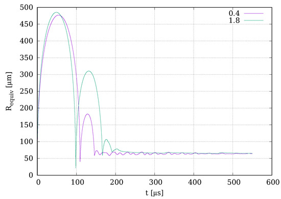
Figure 2.
Equivalent radius, , versus time for and 1.8. The flow-field maps are given at times either or , when the oscillations of the bubble have ceased. The liquid, however, is still flowing.
It is seen in Figure 2 that with the bubble model applied (Equations (1)–(6)), the bubble exhibits rebounds with different strengths. However, in any case, the bubble oscillations have ceased after about 550 µs. Nevertheless, the liquid flow induced persists and may form liquid flow structures. The most prominent ones are liquid vortices of different kinds. As the vortices fully develop only long after the bubble oscillations have ceased, most vortex plots are given at = 550 µs after bubble generation. To decide about the type of vortex in critical cases, the vortices at = 1000 µs are given. The decision on the vortex type at 1 ms is called the 1 ms criterion.
2.4. Flow-Field Visualization
As indicated in Section 1, there exist different methods to experimentally visualize liquid flows. With the PTV and/or PIV method, not only the flow can be visualized, but also the velocity field can be measured. The particles used in PTV and PIV can either be reflective or fluorescent. Their location and motion is followed photographically or holographically. For reflecting particles applied in the flow around bubbles, see, e.g., Lauterborn and Vogel [11], Vogel et al. [13] and Lauterborn and Kurz [53], and for fluorescent particles, see, e.g., Kröninger et al. [26] and Reuter et al. [30]. From consecutive illumination flashes, velocity vectors can be derived from the illuminated particles.
A more compact method is dye advection applied to experiments, where the liquid is at rest in the beginning: An ink-colored liquid layer is put into the liquid sample at the start of the measurement, which is then distorted by the flow to give a flow-field map when photographed at times wanted.
When post-processing the data of a time-varying velocity field, gained by either experiment or numerical simulation, the dye advection method can be set up a posteriori by digitally coloring the liquid and advecting the color with the corresponding, calculated tracer trajectories. When the dye is injected also at different times , this is termed dye injection [31]. In the case of a laser-induced cavitation bubble it is, however, more suitable to inject the color only at time zero, since the dynamics is very fast.
A similar method is used here with digitally colored liquid layers, stratified parallel to the flat surface of the solid in a quiet liquid at bubble generation, whereby the liquid flow is not obtained from measurements but from numerical calculations. The numerical dye or, in OpenFOAM-terminology, passive scalar is advected passively with the velocity field by an advection equation [51]:
is initiated varying only in direction orthogonal to the solid surface and thus as stratified color layers when applying an adequate color map to the values of . The validity of the method was investigated in Koch [8]. The initial data of are set to:
for the center of the bubble in at . With these initial data, the color layers extend from the solid surface, , to . For different , hence different , the thickness of the color layers is adapted.
Figure 3 shows an example of one type of a liquid vortex after the expansion, collapse and rebounds of a bubble close to a solid boundary. The vortex is visualized from the simulation with the dye advection method via Equation (10). The stratified colors from bottom to top are: whitish, dark blue, black, green, light blue and purple. The bubble oscillation has long gone, but the liquid set into motion still persists and forms the large vortex shown at 550 µs after bubble generation. The initial bubble is modeled by a small sphere of high pressure, which is given by the small, white sphere at the center of the large, transparent sphere in the cut through the axis of symmetry. The transparent sphere with radius is copied in to show the maximum extension the bubble would reach in an unbounded liquid. It gives an impression of the normalized distance (smaller than one, here = 0.8) by crossing the solid boundary and lets us imagine that the actual bubble must have undergone a (rotationally symmetric) distortion during expansion by the existence of the solid surface.
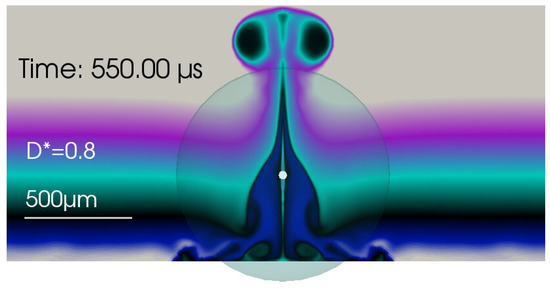
Figure 3.
Example of a numerically obtained dye advection map as used in the present article. Shown is the bubble-induced vortex flow after jet formation, the second collapse and further rebounds for up to the state at = 550 µs. The small white sphere denotes the initial bubble size and position. The large, transparent, filled circle (a sphere in 3D) denotes the maximum extension the same bubble would attain in an unbounded liquid. With a boundary, the maximum extension is reached at . The lower boundary of the figure coincides with the surface of the solid. It is cut perpendicular to the surface, including the axis of symmetry. The frame size can be seen from the size of the transparent sphere of radius and from the bar denoting 500 µm.
For this type of diagram, also, the motion direction of the vortex can be inferred from the color it carries. In the given case of , the motion is upwards for the large vortex. The near-boundary liquid is carried upwards into the free liquid. The colors in the large ring vortex from inside of the vortex ring to outside are dark blue, black, green, light blue and violet.
Figure 4 shows the same vortex as in Figure 3 but in a different way with the vorticity (z-direction pointing toward the reader) and superimposed flow-field direction arrows to show the actual flow field at . In this case, the flow of the large vortex is upwards (away from the solid boundary) at the axis of symmetry and redirected back downwards at larger distances from the axis to form a large-scale, dipole-like vortex flow. Due to the axial symmetry, the rotation is clockwise (in this example) in the right half of the cut and anti-clockwise in the left half. From the flow-field direction arrows and the vorticity colors, it is seen that there are several small-scale ring vortices present at the solid boundary and one with opposite turning direction between the solid surface and the large-scale vortex.
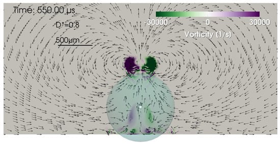
Figure 4.
Same vortex as in Figure 3 but in a different presentation with vorticity and superimposed flow-field direction arrows. It is cut perpendicular to the surface, including the axis of symmetry. The lower boundary coincides with the surface of the solid.
The two forms of flow-field visualization as presented in this section will be used in the following to characterize the vortices found in laser-generated bubbles. They give different insights as to the properties of the vortices. The dye advection maps incorporate the flow up to the plot time, and the vorticity maps with superimposed flow-field direction arrows are a snapshot of the vortex at plot time. Thus, they carry different information and add to one another.
3. Results
The color-layer mixing dynamics of the dye advection is explained by means of a time series. Afterwards, two types of vortices in the case of a bubble close to a solid boundary are introduced with their different rotation and translational motion directions (Section 3.2). They coexist throughout the interval of investigated. In a transition interval, they exchange their dominating strength, as given by the modulus of the vorticity, ||, and the spatial extent. As the settling time for the flow field becomes larger, when approaching the transition threshold, the respective simulations were extended to 1 ms since bubble generation. Finally, the numerically found transition interval is compared to the experimentally determined one by Reuter et al. [30] (Section 3.4).
3.1. Color-Layer Mixing Dynamics
The color mixing—as seen in Figure 3 for the bubble at at = 550 µs—shows a complicated structure explained as a large vortex with additional details. The green needle along the axis of symmetry, for instance, can be attributed to the motion of the bubble and its surrounding liquid from the green layer toward the solid and the squeezing back of the green liquid toward the axis of symmetry in the course of collapses and rebounds. This will become clear when the development of the flow is depicted in a time series of dye advection maps in Figure 5. The first bubble collapse produces a liquid microjet toward the solid. The jet then drives liquid toward the solid boundary. Liquid from the green layer around the axis of symmetry is transported downwards by the jet (frames 2–6, Figure 5). Liquid from the light blue and black color layers are sucked into the jet as well. In frame three of Figure 5, a ring sheet (in 3D) of liquid shoots into the bubble. This phenomenon, termed annular nanojet, has been described in Lechner et al. [43] and the reader is referred to this reference for details. After impact at the solid surface, liquid from the jet spreads along the surface, as seen in frame 4. The reason as to why the final motion of the liquid is directed into the liquid bulk is the inversion of motion by the second bubble collapse and only small rebound (frames 5–9). The second collapse (frame 5) starts at the outer rim of the gas torus, and the flow is directed inwards toward the axis of symmetry (frames 6 and 7). The rebound (frame 7) of the gas phase then takes place from near the solid boundary with a layer of liquid in between. The second rebound is of small amplitude (see Figure 2) and is not able to stop the inflow of liquid from the second collapse. The former downwards-oriented part of the light-blue and green layer is now squeezed to the axis by the inward liquid motion from the second collapse and necessarily pushed upwards together with all layers except the whitish one. The whitish layer has been pushed so far away from the axis of symmetry by the surface flow from other layers that it no longer takes part in the essential dynamics.
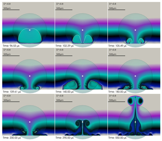
Figure 5.
Time series of the vortex for at selected times. The bubble interior is colored green to show that the bubble is generated in the green liquid layer. The outline of the bubble is given in white. The series starts with the first collapse (first four frames), proceeds with the second collapse from 140 µs onwards, and ends with the second rebound (last two frames), where the vortex is generated. The remaining gas fractions from the second rebound are of too small volume to be seen. Compare the decaying bubble oscillations in Figure 2. The lower boundary of the frames coincides with the surface of the solid.
Additionally, several small-scale vortices are seen along the surface of the solid (see also Figure 4, the vorticity diagram). Prominently seen is the small bubble vortex following the jet impact during first collapse. It spreads along the surface by the ongoing inflow of liquid (frame 4 at time 109.61 µs in Figure 5). The complete set of vortices found is described next.
3.2. The Two Types of Vortices and Their Origins
In axial symmetry, there are two types of bubble-jet-induced liquid vortices close to a solid boundary. Either the liquid flow through the vortex center along the axis of symmetry is upwards, away from the boundary—“up-vortex” (motion of the forming vortex also upwards as can be guessed from the color advection or seen from a succession of frames), or downwards, toward the solid boundary—“down-vortex” (motion of the forming vortex downwards as demonstrated later). An example of an up-vortex is given in Figure 6, and an example of a down-vortex is given in Figure 7. The figures are a combined version of a flow and a vorticity map, as shown separately in Figure 3 and Figure 4. Because of the axial symmetry, a half part of the cut is sufficient.
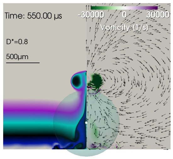
Figure 6.
Up-vortex at = 550 µs for . The dominating large-scale flow is clockwise. Left part: Flow-field map from colored liquid layers. Right part: Vorticity map according to Equation (9) with superimposed flow-direction arrows. Small-scale vortices are seen along the solid surface. The small white sphere denotes the initial bubble size and position. As before, the large, transparent, filled circle (a sphere in 3D) denotes the maximum extension the numerical bubble would attain in an unbounded liquid. It is cut perpendicular to the surface, including the axis of symmetry.
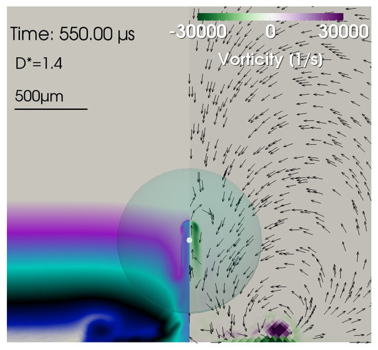
Figure 7.
Down-vortex at = 550 µs for . The dominating large-scale flow is counter-clockwise. The vortex is located near the solid surface and is best seen in the right part in its extension. One small-scale up-vortex is located near the axis of symmetry.
The two types of vortices can further be distinguished by the second type of visualization, as presented in Figure 4 by a toroidal rotation criterion. When in the cut only the right half part of the flow-direction map is considered, then the flow around an up-vortex is “clockwise”. Figure 6 shows an example of a vortex with clockwise rotation of the liquid, i.e., an up-vortex. Note that the rotation direction is only valid for the right part of the cut through the torus vortex. It is known that a ring vortex in an unbounded liquid propagates in the direction of the flow along its axis (see, e.g., Fraenkel [54]). When the vortex axis coincides with the axis of symmetry in an axially symmetric setting, then for a single vortex, the translational motion is upwards—using the terms introduced in the present work—when rotating clockwise, hence downwards when rotating counter-clockwise. However, when vortices come in larger numbers and are densely packed, the rotation criterion is best suited to characterize the type of vortex in an axially symmetric setting.
In Figure 7, an example of a down-vortex is given with its counter-clockwise rotation for = 1.4. It is located near the solid surface. A small, locally confined region with clockwise rotation is seen at the axis of symmetry near the location of bubble generation (the small white circle), too.
The temporal dynamics of the down-vortex generation are shown in the montage in Figure 8 for a bubble at . The main difference in the dynamics compared to the ones for the up-vortex in Figure 5 is the sequence of the bubble shape in the first rebound and second collapse. Here again, flow focusing isthe main driving force [5,55]. Flow focusing is the phenomenon generating the strongest acceleration where interface curvatures are highest. When comparing frame 5 ofFigure 5 to frame 6 of Figure 8, it is noted that the curvature of the torus bubble during the second bubble maximum volume and onset of the second collapse is highest at the outer rim for the up-vortex case, and the curvature is highest in the inner region for the down-vortex case. Therefore, the fluid motion is accelerated highest toward the axis of symmetry in case of the up-vortex, and it is accelerated outwards in case of the down-vortex during the second bubble collapse.
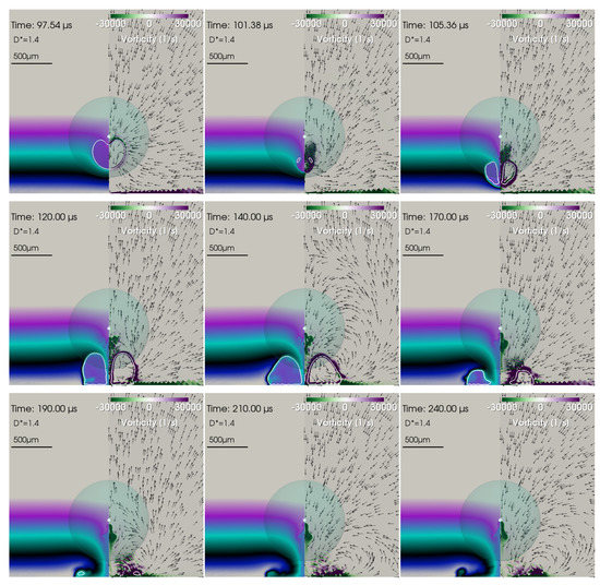
Figure 8.
Time series of the down-vortex for at selected times. The bubble interior is colored violet to show that the bubble has been generated in the violet layer. The outline of the bubble is given in white. The series starts with the first collapse (first two frames) and ends with the forming of the down-vortex after the second collapse (last three frames).
The vortices are dynamical objects that may move and/or change their form. Up-vortices move upwards away from the solid boundary, while down-vortices move toward the solid boundary. Reuter et al. [30] use the motion criterion for classification and call the upwards moving vortices “free vortices” and the downwards moving vortices “wall vortices”. The authors introduced a third status as well, tagged “no vortex”, when neither an up-vortex nor down-vortex was observed within experimental uncertainties. However, in the numerical simulations presented here, it becomes evident that the vortices are always present after the bubble oscillations have ceased. The difference is only in the intensity of the vorticity. In fact, both types of vortices are generally present. It is the ratio of their respective intensities that determines the macroscopic diagnosis made by an observer. An example is given in Figure 9 for . The clockwise rotation direction indicates an up-vortex, while the vortex does not seem to have moved upwards up to = 550 µs but is located away from the boundary. There, the flow rather rolls up, as seen in the left part of the plot. The extension to = 1 ms indicates a vortex with very slow motion upwards, confirming the classification of an up-vortex by its rotation direction from one frame only.
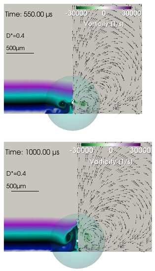
Figure 9.
Up-vortex at according to the clockwise flow at the time instants = 550 µs and 1 ms. The dominating large-scale flow is clockwise, but the up-vortex does not depart upwards like previous up-vortices away from the surface of the solid (see the left part of the left frame and the depression of the green layer downwards). However, it very slowly moves upwards when comparing with a longer time scale ( = 1 ms) as predicted from the rotation direction and the flow upwards along the axis of symmetry already in the left part of the left frame.
3.3. Survey of Vortex Structures in Dependence on
The aim is to find the (dominating) vortices for 0.4 1.8 and whether they are up-vortices or down-vortices. The vortices for the values and 1.4 were already given in Figure 6, Figure 7 and Figure 9. The flow maps for the -values of 0.6, 1.0 and 1.2 are given in Figure 10, Figure 11 and Figure 12, respectively, and in Figure 13 for = 1.6 and 1.8. It is seen that up to = 1.2, the up-vortices dominate (clockwise rotation). For the values of higher than or equal to 1.4, the turning direction of the dominating vortex changes by fading of the up-vortex and by the increasing in strength and extent of the down-vortex. The result is a down-vortex with its counter-clockwise rotation and a location close to the solid surface (Figure 7 and Figure 13).
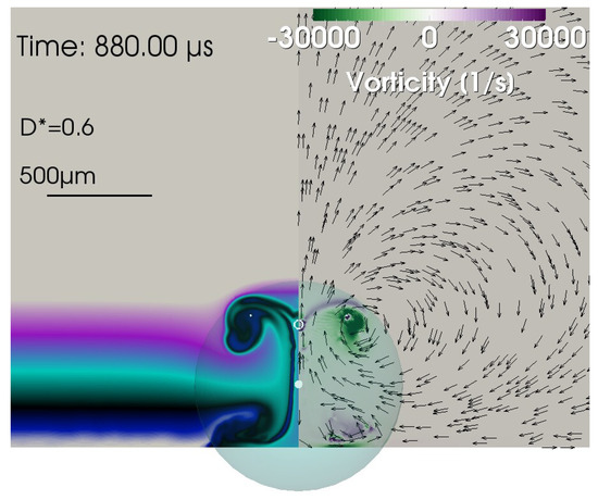
Figure 10.
Up-vortex at = 880 µs for . Small-scale down-vortices are present below the bubble near the solid surface as seen from the color in the vorticity map. Liquid from the green layer has both been advected upwards as well as downwards.
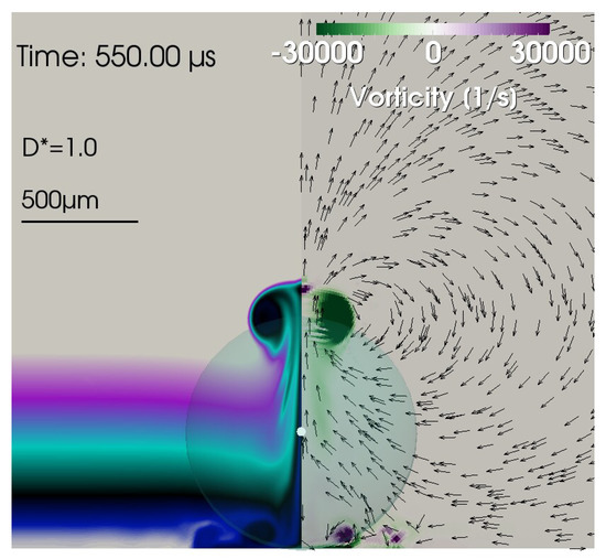
Figure 11.
Up-vortex at = 550 µs at . Localized, small-scale down-vortices are seen below the bubble near to the surface from the color depression downwards and in the flow direction field.
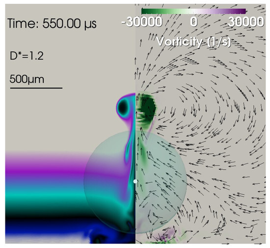
Figure 12.
Up-vortex at = 550 µs for . It is the dominating vortex with its clockwise rotation direction.
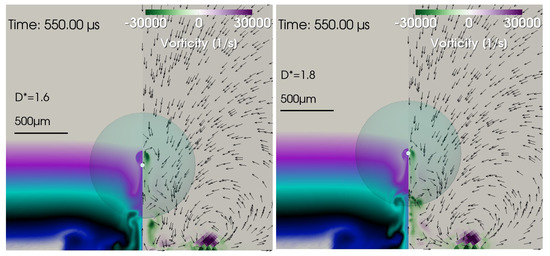
Figure 13.
Down-vortices near the wall at = 550 µs for and 1.8. They are the dominating vortices with counter-clockwise rotation direction.
3.4. The Transition Interval
To better locate the change in the vortex rotation direction from clockwise (up-vortex) to counter-clockwise (down-vortex), the interval 1.2 1.4 was scanned in steps of . The result is presented in Figure 14, Figure 15, Figure 16 and Figure 17 for the transition interval from dominating clockwise rotation to dominating counter-clockwise rotation. The simulations have been extended to = 1 ms, as a unique rotation direction obviously needs time to settle near the transition threshold (1 ms criterion). It is seen that the dominating rotation direction is clockwise at = 1.27 and up to = 1.29 and counter-clockwise at 1.35 and for further values of . A quite sharp transition interval is found between = 1.30 and 1.34. At , it seems that both rotation directions are of equal strength, and thus, there is no overall flow field rotation, and the vortex region is locally confined.
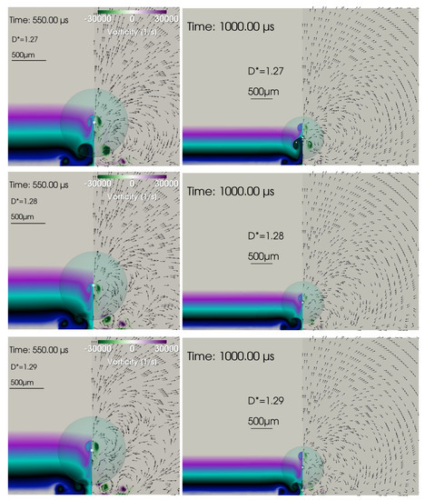
Figure 14.
Up-vortices and down-vortices at and at = 550 µs and 1 ms. At least three clearly visible vortices are generated with two strong up-vortices and only a small down-vortex.
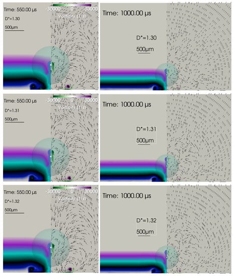
Figure 15.
Up-vortices and down-vortices at and at = 550 µs and 1 ms.
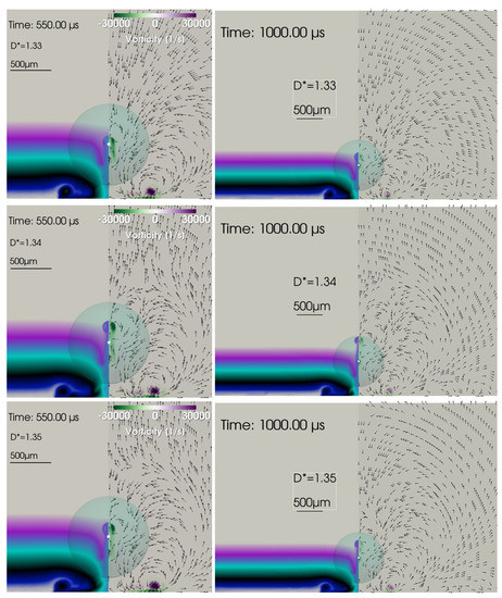
Figure 16.
Up-vortices and down-vortices at and 1.35 at = 550 µs and 1 ms. The large-scale flow changes from clockwise ( = 1.30) to counter-clockwise ( = 1.34) according to the 1 ms criterion).
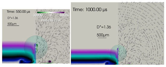
Figure 17.
Up-vortices and down-vortices at at = 550 µs and 1 ms.
Up- and down-vortices of about equal strength coexist. As increases, the up-vortices gradually become slower in their upward motion. A closer inspection of the vortex structure reveals that a coexistence of up- and down-vortices is always the case for the -values studied. It is the large-scale rotation direction that changes between = 1.30 and 1.34. The region of the fading up-vortex has a surrounding clockwise flow field of fading extent superimposed on the counter-clockwise overall flow field from onwards.
3.5. Comparison with Experiments
The numerical findings are compared to the experimental findings of Reuter et al. [30] in Figure 18 and Figure 19.
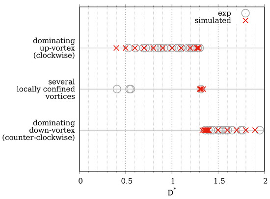
Figure 18.
Comparison of numerically obtained vortex types (red crosses) to experiments by Reuter et al. [30] (gray circles). An excellent agreement is found. The approximation is assumed.
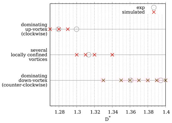
Figure 19.
Comparison of numerically obtained vortex types (red crosses) to experiments by Reuter et al. [30] (gray circles). Magnification into the transition interval. The numerical transition interval is found to be . The experimental transition interval was found to be . The approximation is assumed.
Reuter et al. [30] use a different definition for the normalized distance, , from the one used here, . In the experiment, it is impossible to obtain the maximum radius in the unbounded liquid of the bubble just generated if the current setup contains restrictive objects or dimensions. Therefore, instead of using (refer to Equation (1)) corresponding to the maximum radius of the same bubble in an unbounded liquid, the apparent maximum radius from the measurement was taken, resulting in a , meaning the radius of a sphere with equivalent volume. The precise algorithm of how and were extracted from the measurement data is not clear from the publication. Here, it was decided to plot the data from Reuter et al. [30] as if the relation would hold, which is assumed to be justified for , where fast-jet dynamics are not present yet. The data points from the experiment are plotted with a larger diameter to account for the uncertainty of that assumption.
Reuter et al. [30] discern between three types of vortices: the free vortex, the wall vortex and “no vortex” according to their translational motion. No vortex then means no discernible vortex motion. Here, only two categories of vortices are introduced: the up-vortex and the down-vortex according to their rotation direction. Usually, a free vortex is an up-vortex and a wall vortex is a down-vortex. There is no correspondence to a no-vortex. Using the derived knowledge from the present work, the terminology was adapted to the notation of the rotation direction, up- or down-vortex and whether the vortex propagation velocity nearly vanishes (“several, locally confined”).
When comparing the experimental data points with the numerical ones, an excellent agreement is found. In particular, the numerical transition interval () fits perfectly into the experimental transition interval , where Reuter et al. [30] could find no definite signs for a free or wall vortex.
4. Discussion
An oscillating bubble is an object with long-range interaction forces. In the spherically symmetric case of a free bubble in an infinite, incompressible liquid, it is the breathing mode of the oscillation that leads to a spherically symmetric, quadratically decaying liquid motion. Thus, in principle, the interaction range is infinite. For numerical calculations in single-bubble dynamics, this means that the boundaries must be sufficiently far away from the bubble. It has been found that the boundaries should be at least about 100 times the maximum extension of a spherical cavitation bubble away in order to not significantly alter the dynamics [37] and for numerical convergence reasons [8].
In the non-spherical case with boundaries nearby, the dynamics is totally different with its liquid jet and vortex formation. However, even in a free liquid, jet formation occurs when the liquid is not in a spherically symmetric condition, as for instance with pressure gradients in a gravitational field [56,57] or in a standing acoustic field [58]. As non-spherical conditions prevail in nature and applications, the study of the flow in non-spherical cases is of general interest. There are an infinite number of non-spherical cases. The most important one from a technical application standpoint (cleaning and erosion) is the case of a bubble near a surface or surfaces with the special case of a plane solid surface. There are only a few experimental studies on the flow in this case, in particular on the flow vortices. The, at the time being, most advanced experimental study on vortex formation is from Reuter et al. [30]. Since then, numerics has improved significantly and now is capable of modeling and simulating practically any non-spherical case.
In the present work, the liquid motion of a bubble near a plane solid surface is studied numerically for several distances of the bubble from the solid boundary. A bubble with a radius of 500 µm in an unbounded liquid has been chosen. The focus is on the vortices—generated by the liquid jet, torus bubble collapse, rebound and the further decaying oscillations—and their long-term behavior with respect to translational motion and rotation direction. The experimentally found two types of vortices could be confirmed numerically, which are here called the up-vortex and down-vortex. Both types are present simultaneously with one type being dominant in strength and extent. In a transition interval, one type ceases and the other type takes over. The transition interval is located at . It lies inside the experimentally found transition interval of [30]. The two vortex types can be discerned by the rotation direction of the flow (see Section 3.3 and Figure 6 and Figure 7). The flow needs some time to develop and settle to a dominant type. Therefore, the numerical transition interval was determined at 1 ms after bubble generation, i.e., a long time after jet formation compared to the collapse time of about 50 µs (see Figure 2).
The origin for the two main vortex propagation directions, upwards and downwards, has been determined to be flow focusing during the second collapse (refer to Section 3.3 and Figure 5 and Figure 8). High bubble interface curvatures are accelerated faster than low curvatures. The torus–bubble cross-sectional shape (volume) after rebound determines the fluid acceleration direction afterwards.
It is assumed that there must be a connection to the dynamics of the bubble and therewith to the erosion of the surface. The erosion pattern strongly alters with the normalized distance in a characteristic manner as does the bubble dynamics. Both show a strong correlation: erosion is only observed for bubbles collapsing directly in contact with the solid. In the interval around the transition, the erosion is strongly increased (Figure 21 [59]). Already at and higher values, the first collapse does not take place directly at the solid boundary anymore; however, in this aforementioned interval, the second collapse is from a torus bubble directly sitting on the surface. Correspondingly, the erosion pattern is ring-like as observed. Wang et al. [60], with a modified BIM model (boundary integral method), was able to numerically follow the bubble oscillations to the second collapse, when it becomes a torus bubble sitting on the surface. The torus size coincided with the damage ring found by Philipp and Lauterborn [59]. Moreover, at = 1.2, the bubble lifts off the surface after the second collapse, and the third collapse takes place away from the surface just like the first collapse before and like the following ones (Figure 2f [59]). This is observed in the simulation of the present work for the same , too. This is in correspondence with the final up-vortex, here carrying a larger gas fraction with it.
Now, when looking at the bubble dynamics in the experiment for = 1.4, it is seen that after the second collapse, the torus bubble does not lift up but rather stays at the surface and spreads there. Thus, the flow of liquid connected with it is downwards, and it is in correspondence with the down-vortex. The transition is well in between 1.2 < < 1.4. Tomita and Shima [61] measured the maximum collapse pressure for the second collapse at = 1.3. This is an extremely interesting experimental finding in view of the numerical findings here. At = 1.3, the transition from a dominating up-vortex to a dominating down-vortex takes place. Simultaneously, Philipp and Lauterborn [59] found the maximum erosion around this . Thus, there seems to exists a correlation between all four quantities/events: maximum pressure, maximum erosion, second collapse (directly at the solid surface for = 1.3), and the transition. The erosion is increasingly diminished for growing > 1.4 by the growing distance of the relevant events (jet impact pressure and bubble collapse pressure) from the solid surface. At about = 2.0, erosion ceases.
At first sight, it could be expected that the jet flow dominates the more the nearer the bubble collapses to the surface, i.e., at small . However, the example of shows that it is not the case: the final flow is upwards. The reason is that there is a competition between the jet flow from the first collapse and the subsequent rebound and second collapse. The time when the bubble touches the solid boundary is always between the first bubble volume minimum and the second maximum for in the investigated interval of . The higher the value for , the later the bubble touches the solid boundary during the first rebound. It seems to matter how much of the rebound momentum takes place along the solid boundary in order to create a flow reversal during second collapse against the inflow from the jet from the first collapse.
For values below = 0.4, the transition to the fast jet is entered with the fast-jet region below ≈ 0.2. These values are left for further studies in view of their special dynamics and jet production mechanism.
5. Conclusions and Outlook
Vortex dynamics following the jet formation of a bubble expanding and collapsing close to a plane solid boundary is studied numerically. Two types of vortices, up- and down-vortices, exist simultaneously with one type dominating in strength and extent. The interval of from 0.4 to 1.8 has been studied. In the interval, a transition from one type to the other takes place with the up-vortices below and the down-vortices above the transition value. The numerically found transition value lies well in the experimentally found transition interval.
The benefit of the comparison of the numerical results to the experimental results is threefold. Firstly, the stability of the solver with its extensions (see Appendix A–Appendix C) is demonstrated for long calculation times. Secondly, the perfect agreement with the experiments validates the solver for the cases studied, in particular long-term vortex formation. Thirdly, it is shown that the main bubble and vortex dynamics are essentially axially symmetric, even if this is not evident from the experiments (2D projections).
Moreover, by comparison of different works, a correlation between erosion, bubble dynamics, pressure at the solid and vortex dynamics has been established in the range 0.4 < < 1.8, which is valid for a bubble with a maximum radius of 500 µm. Only bubbles collapsing in direct contact with the solid cause erosion.
With these results, new tasks come into reach: for instance, long-term studies of acoustic bubble oscillations with extreme bubble surface deformations near solids. Further bubble mass control methods may be necessary for this case. Then, studies as to the growth to a stable state or to instability in dependence on the acoustic pressure amplitude can be conducted and compared with experiments. Long-term bubble interaction studies may profit from the knowledge of the large spatial extent of the liquid vortex motion and the longevity of the vortices. Thus, the present work opens up a large area for future research.
Author Contributions
Conceptualization, R.M.; Software, M.K. and C.L.; Validation, C.L.; Formal analysis, W.L. and C.L.; Investigation, M.K.; Resources, R.M.; Data curation, M.K. and C.L.; Writing—original draft, M.K. and W.L.; Writing—review & editing, W.L., C.L. and R.M.; Visualization, M.K.; Supervision, W.L. and R.M.; Project administration, R.M.; Funding acquisition, R.M. and C.L. All authors have read and agreed to the published version of the manuscript.
Funding
The work was supported in part by the Deutsche Forschungsgemeinschaft (DFG, German Research Foundation) under projects Me 1645/8-1 and Me 1645/8-3 and the Austrian Science Fund (FWF) (Grant No. I 5349-N).
Data Availability Statement
The research data of this work is available under the following repository link of the University of Göttingen: https://doi.org/10.25625/4PPDVQ (accessed on 18 May 2023).
Acknowledgments
The authors thank the Cavitation Bubble Dynamics Group at the Drittes Physikalisches Institut, Universität Göttingen, for many inspiring discussions. The authors also thank the workers of the workshops and the IT support at the Drittes Physikalisches Institut for their constant support. The publication cost support by the Georg-August University of Göttingen under the Institutional Open Access Program (IOAP) is gratefully acknowledged.
Conflicts of Interest
The authors declare no conflict of interest.
Appendix A. Mesh, Initial Conditions and Boundary Conditions
The simulations are carried out in axial symmetry. A sketch of the mesh is shown in Figure A1. A similar type of mesh has been introduced already in Koch et al. [37]. The parameters and details since then have constantly been adapted with further experience.The idea is to align the cells as much as possible to the bubble interface, i.e., a polar orientation with apex at the initial bubble center, while at the same time dissipating the shock wave in the outer regions and avoiding a high total cell amount for the whole mesh. The mesh center core region () consists of a rectangular block with cells in Cartesian orientation and a homogeneous minimum cell size of . The follow-up region () serves as the transition region from Cartesian to polar cell orientation. The next region consists of cells with an edge aspect ratio almost equal to 1. Because of the spreading in the -direction, the cell closest to X must have an edge length that is by a factor of larger than the edge length of the cell closest to Xii (see calculation in Koch [62]). is called grading. In the last region , the grading that is neccessary to maintain a cell edge ratio of unity is exaggerated by a user-defined grading factor to dampen the outgoing shock wave. The geometric parameters for the investigation were chosen as given in Table A1.

Figure A1.
Sketch of the mesh with axial symmetry and polar cell orientation except for the immediate surrounding of the initial bubble, which is Cartesian. Not to scale.
Figure A1.
Sketch of the mesh with axial symmetry and polar cell orientation except for the immediate surrounding of the initial bubble, which is Cartesian. Not to scale.


Table A1.
Setup parameters for the mesh. .
Table A1.
Setup parameters for the mesh. .
| Xi | Xii | X | XF | Grading Factor | Amount of Cells | |
|---|---|---|---|---|---|---|
| 2 µm | 4 | 30,000 |
The boundary conditions are set as follows: the wall boundary has a no-slip condition for and a vanishing normal gradient for as well as for p. The mesh is set to be a wedge mesh, meaning axial symmetry in OpenFOAM terms. The outer boundary is set to be wave transmissive for p [63,64], pressure-inlet-outlet-velocity for U and vanishing normal gradient for . The pressure-inlet-outlet-velocity condition, in general, specifies zero normal gradient. In case of inflow, the tangential component is set to zero [65].
The initial data for the bubble are set in the following way. The liquid is at rest at ambient pressure . The user-given initial equilibrium radius , the starting radius of the bubble and the ambient pressure determine the energy of the bubble [66]. At a later stage during calculation, condensation effects are accounted for by reducing the equilibrium radius to , as described later in Appendix D. With the user-given set of parameters, the initial gas region is discretized on the mesh. The discretized gas volume is computed and transformed from axisymmetric to a 3D volume , with the half opening angle of the wedge mesh. With that volume, the pressure that produces the same potential energy of the bubble as the ideal one from the user-given parameters is calculated. This pressure is usually less than 1% different from the ideal one, but this adaption is necessary for grid convergence studies. The maximum bubble radius and collapse time sensitively depend on the initial pressure when accuracy higher than 5% is anticipated. The precise algorithm is as follows:
Table A2.
Fluid properties entering the calculation. is the specific gas constant of air.
Table A2.
Fluid properties entering the calculation. is the specific gas constant of air.
| Fluid | [] | [] | ; | B [Pa]; [] |
|---|---|---|---|---|
| liquid | 998.2 | 7.15 | ||
| gas | derived | 1.4 | 287.0 | |
| [] | [Pa] | [K] | ||
| 0.0725 | 101315 | 293.15 |
Appendix B. Time Stepping
In the present work, the flow patterns are of interest that persist long after the bubble oscillations have ceased. The simulation therefore has to pass a long period of time where the dynamics are not violent anymore. Hence, a suitable time stepping is important for the different phases of the bubble dynamics for a trade-off between numerical stability and computational effort.
The Courant number Co is calculated to determine the time step size for adaptive time stepping. It is defined as the spatial maximum of the ratio of the local flow speed at location to the maximum resolvable flow speed by the spatial and temporal discretization ():
Not only the Courant number Co of the advective flow but also the acoustic Courant number and the flow Courant number of the bubble interface, , were considered. The latter two are formed with , where c denotes the local speed of sound, and the flow velocity at the interface , respectively, instead of the velocity .
The upper limits of the three criteria are set to the values given in Table A3. There is also the restriction for the size of the time step for all times, . The is set to 50 ns or 500 ns. Since the vortices fully develop very late in the bubble process, the simulation needs to run for a long time. Therefore, a script was written to supervise the calculation and change the time stepping for times when the fast bubble collapses are over. The changes made are given in Table A3.
Table A3.
Time stepping of the simulations to save calculation time. is the bubble radius at time t and is the radius at rest.
Table A3.
Time stepping of the simulations to save calculation time. is the bubble radius at time t and is the radius at rest.
| time | for | ||||
|---|---|---|---|---|---|
| 0 s–120 µs | 0.2 | 0.2 | 8 | 0.3 | |
| 120 µs–200 µs | 0.2 | 0.2 | 30 | 0.01 | |
| 200 µs–end | 0.4 | 0.4 | 100 | 0.01 |
Appendix C. Bubble Mass Correction Methods
It was noted already in Miller et al. [67] and Koch et al. [37] that due to the segregated nature of the solver, the mass of the bubble undergoes an error over time. We apply two versions of compensation. Both of them are applied after the last iteration of the pressure equation.
Appendix C.1. Global Mass Correction
The first approach has been described in Koch et al. [37]. The density in each cell of the gas phase simply is multiplied by the ratio of the initial bubble mass to the current bubble mass:
This approach has been validated by comparison to the Gilmore model [68] and to experimental data also in axial symmetry in Koch et al. [37]. It has been proven to work very well until the first collapse and slightly longer. The disadvantage is that when the bubble becomes fragmented, each of the fragments is treated the same regardless of the local mass errors of the fragments.
Appendix C.2. Local Mass Correction
The second approach aims to compensate the error where it occurs. After the last iteration of the pressure equation, the continuity equation for the gas is reconsidered in the form
and solved for the field . The gas density is obtained from the field by division by , where is a copy of the field with
in order to avoid division by zero. This approach has been validated by a direct comparison of simulations in axial symmetry and full 3D to experiments in Koch [8] and Koch et al. [6].
Appendix D. Bubble Mass Control
In order to model a strong collapse of the bubble, as seen in the experiments, the following procedure is applied. The phenomenon of laser-induced breakdown to produce a bubble is not modeled in the present work. Instead, an initial bubble of high internal pressure is taken that expands to the experimental maximum radius. The condensation of the vapor part in the bubble is modeled by a reduction of the radius at rest of the bubble, . Hentschel and Lauterborn [69] stated that good agreement between the Gilmore model and experiments is found when the equilibrium radius of the bubble is reduced by 60 % at the time when the bubble is at its maximum radius. In the present work, this approach was incorporated by a linear reduction of from to in the time interval between and :
The density of the bubble is changed in the same manner by a global mass correction step (see Appendix C.1) after the new has been determined:
The values of and in this work are chosen as follows: for fixed , is a parameter that is varied for different initial bubble energies and hence different maximum radii the bubble expands to. Akhatov et al. [40] gave experimental data on the rebound radius compared to the maximum radius of a bubble in unbounded liquid for a total of 16 experiments. When fitting these data with the present code, the following relation is found:
Hentschel and Lauterborn (see Figure 6 [69]) found that . A comprehensive analysis on the ratio of the first rebound radius to is given in Liang et al. (see Figure 15 [45]), where it is also mentioned that this ratio depends on the focusing quality of the optics producing the plasma. In the present work, was chosen to be fixed at .
This method to reduce the gas content during simulation has been proven to work well by comparison with experiments, as shown here and previously in Koch et al. [37].
References
- Plesset, M.S.; Chapman, R.B. Collapse of an initially spherical vapour cavity in the neighbourhood of a solid boundary. J. Fluid Mech. 1971, 47, 283–290. [Google Scholar] [CrossRef]
- Blake, J.R.; Keen, G.S.; Tong, R.P.; Wilson, M. Acoustic cavitation: The fluid dynamics of non-spherical bubbles. Philos. Trans. R. Soc. Lond. Ser. A 1999, 357, 251–267. [Google Scholar] [CrossRef]
- Tong, R.P.; Schiffers, W.P.; Shaw, S.J.; Blake, J.R.; Emmony, D.C. The role of ‘splashing’ in the collaspe of a laser-generated cavity near a rigid boundary. J. Fluid Mech. 1999, 380, 339–361. [Google Scholar] [CrossRef]
- Supponen, O.; Obreschkow, D.; Tinguely, M.; Kobel, P.; Dorsaz, N.; Farhat, M. Scaling laws for jets of single cavitation bubbles. J. Fluid Mech. 2016, 802, 263–293. [Google Scholar] [CrossRef]
- Lechner, C.; Lauterborn, W.; Koch, M.; Mettin, R. Jet formation from bubbles near a solid boundary in a compressible liquid: Numerical study of distance dependence. Phys. Rev. Fluids 2020, 5, 093604. [Google Scholar] [CrossRef]
- Koch, M.; Rosselló, J.M.; Lechner, C.; Lauterborn, W.; Eisener, J.; Mettin, R. Theory-assisted optical ray tracing to extract cavitation-bubble shapes from experiment. Exp. Fluids 2021, 62, 1–19. [Google Scholar] [CrossRef]
- Lechner, C.; Lauterborn, W.; Koch, M.; Mettin, R. Fast, thin jets from bubbles expanding and collapsing in extreme vicinity to a solid boundary: A numerical study. Phys. Rev. Fluids 2019, 4, 021601. [Google Scholar] [CrossRef]
- Koch, M. Laser Cavitation Bubbles at Objects: Merging Numerical and Experimental Methods. Ph.D. Thesis, Third Physical Institute, Georg-August-Universität, Göttingen, Germany, 2020. Available online: http://hdl.handle.net/21.11130/00-1735-0000-0005-1516-B (accessed on 19 May 2023).
- Reuter, F.; Ohl, C.D. Supersonic needle-jet generation with single cavitation bubbles. Appl. Phys. Lett. 2021, 118, 134103. [Google Scholar] [CrossRef]
- Lauterborn, W.; Hentschel, W.; Timm, R. Ist der Kollapszustand einer Kavitationsblase ein kurzlebiger Wirbelring? (Is the collapse state of a cavitation bubble a short living vortex ring?). DAGA-Fortschritte der Akustik 1981, 8, 457–460. [Google Scholar]
- Lauterborn, W.; Vogel, A. Modern Optical Techniques in Fluid Mechanics. Annu. Rev. Fluid Mech. 1984, 16, 223–244. [Google Scholar] [CrossRef]
- Vogel, A.; Lauterborn, W. Time-resolved particle image velocimetry used in the investigation of cavitation bubble dynamics. Appl. Opt. 1988, 27, 1869–1876. [Google Scholar] [CrossRef]
- Vogel, A.; Lauterborn, W.; Timm, R. Optical and acoustic investigations of the dynamics of laser-produced cavitation bubbles near a solid boundary. J. Fluid Mech. 1989, 206, 299–338. [Google Scholar] [CrossRef]
- Grant, I. Selected Papers on Particle Image Velocimetry SPIE Milestone Series MS 99; SPIE Optical engineering Press: Bellingham, WA, USA, 1994. [Google Scholar]
- Grant, I. Particle image velocimetry: A review. Proc. Inst. Mech. Eng. Part C J. Mech. Eng. Sci. 1997, 211, 55–76. [Google Scholar] [CrossRef]
- Adrian, R.J. Twenty years of particle image velocimetry. Exp. Fluids 2005, 39, 159–169. [Google Scholar] [CrossRef]
- Raffel, M.; Willert, C.; Wereley, S.; Kompenhans, J. Particle Image Velocimetry–A Practical Guide, 2nd ed.; Springer: Berlin/Heidelberg, Germany, 2007. [Google Scholar]
- Nobach, H.; Tropea, C. Improvements to PIV image analysis by recognizing the velocity gradients. Exp. Fluids 2005, 39, 614–622. [Google Scholar] [CrossRef]
- Nobach, H. Optische Messtechnik; Edition Winterwork: Borsdorf, Germany, 2012; ISBN 978-3-86468-206-3. Available online: http://www.nambis.de/publications/omt12.html (accessed on 28 May 2023).
- Schanz, D.; Gesemann, S.; Schröder, A. Shake-the-Box: Lagrangian particle tracking at high particle image densities. Exp. Fluids 2016, 57, 1–27. [Google Scholar] [CrossRef]
- Kähler, C.J.; Astarita, T.; Vlachos, P.P.; Sakakibara, J.; Hain, R.; Discetti, S.; La Foy, R.; Cierpka, C. Main results of the 4th International PIV Challenge. Exp. Fluids 2016, 57, 1–71. [Google Scholar] [CrossRef]
- Sellappan, P.; Alvi, F.S.; Cattafesta, L.N. Lagrangian and Eulerian measurements in high-speed jets using Multi-Pulse Shake-The-Box and fine scale reconstruction (VIC#). Exp. Fluids 2020, 61, 1–17. [Google Scholar] [CrossRef]
- Bolaños-Jiménez, R.; Rossi, M.; Rivas, D.F.; Kähler, C.J.; Marin, A. Streaming flow by oscillating bubbles: Quantitative diagnostics via particle tracking velocimetry. J. Fluid Mech. 2017, 820, 529–548. [Google Scholar] [CrossRef]
- Rossi, M.; Kähler, C.J. Optimization of astigmatic particle tracking velocimeters. Exp. Fluids 2014, 55, 1809. [Google Scholar] [CrossRef]
- Fauconnier, M.; Mauger, C.; Béra, J.C.; Inserra, C. Nonspherical dynamics and microstreaming of a wall-attached microbubble. J. Fluid Mech. 2022, 935, A22. [Google Scholar] [CrossRef]
- Kröninger, D.; Köhler, K.; Kurz, T.; Lauterborn, W. Particle tracking velocimetry of the flow field around a collapsing cavitation bubble. Exp. Fluids 2010, 48, 395–408. [Google Scholar] [CrossRef]
- Kröninger, D.A. Particle-Tracking-Velocimetry-Messungen an kollabierenden Kavitationsblasen (Particle-Tracking-Velocimetry measurements on collapsing cavitation bubbles). Ph.D. Thesis, Drittes Physikalisches Institut, Georg-August Universität, Göttingen, Germany, 2008. [Google Scholar]
- Koch, M.; Rosselló, J.M.; Lechner, C.; Lauterborn, W.; Mettin, R. Dynamics of a Laser-Induced Bubble above the Flat Top of a Solid Cylinder–Mushroom-Shaped Bubbles and the Fast Jet. Fluids 2022, 7, 2. [Google Scholar] [CrossRef]
- Lauterborn, W.; Lechner, C.; Koch, M.; Mettin, R. Bubble models and real bubbles: Rayleigh and energy-deposit cases in a Tait-compressible liquid. IMA J. Appl. Math. 2018, 83, 556–589. [Google Scholar] [CrossRef]
- Reuter, F.; Gonzalez-Avila, S.R.; Mettin, R.; Ohl, C.D. Flow fields and vortex dynamics of bubbles collapsing near a solid boundary. Phys. Rev. Fluids 2017, 2, 064202. [Google Scholar] [CrossRef]
- Jobard, B.; Erlebacher, G.; Hussaini, M.Y. Lagrangian-Eulerian Advection of Noise and Dye Textures for Unsteady Flow Visualization. IEEE Trans. Vis. Comput. Graph. 2002, 8, 211–222. [Google Scholar] [CrossRef]
- Laramee, R.S.; Hauser, H.; Doleisch, H.; Vrolijk, B.; Post, F.H.; Weiskopf, D. The State of the Art in Flow Visualization: Dense and Texture-Based Techniques. Comput. Graph. Forum 2004, 23, 203–221. [Google Scholar] [CrossRef]
- Saini, M.; Tanne, E.; Arrigoni, M.; Zaleski, S.; Fuster, D. On the dynamics of a collapsing bubble in contact with a rigid wall. J. Fluid Mech. 2022, 948, A45. [Google Scholar] [CrossRef]
- Sieber, A.B.; Preso, D.B.; Farhat, M. Dynamics of cavitation bubbles near granular boundaries. JFM 2022, 947, A39. [Google Scholar] [CrossRef]
- Creative Commons. Attribution-NonCommercial 2.0 Generic (CC BY-NC 2.0). Available online: https://creativecommons.org/licenses/by-nc/2.0/ (accessed on 28 May 2023).
- Gschaider, B.; Nilsson, H.; Rusche, H.; Jasak, H.; Beaudoin, M.; Skuric, V. Open Source CFD Toolbox. 2017. Available online: https://sourceforge.net/projects/foam-extend/ (accessed on 19 May 2023).
- Koch, M.; Lechner, C.; Reuter, F.; Köhler, K.; Mettin, R.; Lauterborn, W. Numerical modeling of laser generated cavitation bubbles with the finite volume and volume of fluid method, using OpenFOAM. Comput. Fluids 2016, 126, 71–90. [Google Scholar] [CrossRef]
- Brennen, C.E. Cavitation and Bubble Dynamics; Oxford University Press: Oxford, UK, 1995. [Google Scholar]
- Fujikawa, S.; Akamatsu, T. Effects of the non-equilibrium condensation of vapour on the pressure wave produced by the collapse of a bubble in a liquid. J. Fluid Mech. 1980, 97, 481–512. [Google Scholar] [CrossRef]
- Akhatov, I.; Lindau, O.; Topolnikov, A.; Mettin, R.; Vakhitova, N.; Lauterborn, W. Collapse and rebound of a laser-induced cavitation bubble. Phys. Fluids 2001, 13, 2805–2819. [Google Scholar] [CrossRef]
- Akhatov, I.; Vakhitova, N.; Topolnikov, A.; Zakirov, K.; Wolfrum, B.; Kurz, T.; Lindau, O.; Mettin, R.; Lauterborn, W. Dynamics of laser-induced cavitation bubbles. Exp. Therm. Fluid Sci. 2002, 26, 731–737. [Google Scholar] [CrossRef]
- Lauterborn, W.; Vogel, A. Shock Wave Emission by Laser Generated Bubbles. In Bubble Dynamics & Shock Waves; Delale, C., Ed.; Springer: Berlin/Heidelberg, Germany, 2013; pp. 67–103. [Google Scholar] [CrossRef]
- Lechner, C.; Koch, M.; Lauterborn, W.; Mettin, R. Pressure and tension waves from bubble collapse near a solid boundary: A numerical approach. J. Acoust. Soc. Am. 2017, 142, 3649–3659. [Google Scholar] [CrossRef] [PubMed]
- Supponen, O.; Obreschkow, D.; Kobel, P.; Tinguely, M.; Dorsaz, N.; Farhat, M. Shock waves from nonspherical cavitation bubbles. Phys. Rev. Fluids 2017, 2, 093601. [Google Scholar] [CrossRef]
- Liang, X.X.; Linz, N.; Freidank, S.; Paltauf, G.; Vogel, A. Comprehensive analysis of spherical bubble oscillations and shock wave emission in laser-induced cavitation. J. Fluid Mech. 2022, 940, A5. [Google Scholar] [CrossRef]
- Brackbill, J.U.; Kothe, D.B.; Zemach, C. A Continuum Method for Modeling Surface Tension. J. Comput. Phys. 1992, 100, 335–354. [Google Scholar] [CrossRef]
- Tryggvason, G.; Bunner, B.; Esmaeeli, A.; Juric, D.; Al-Rawahi, N.; Tauber, W.; Han, J.; Nas, S.; Jan, Y.J. A Front-Tracking Method for the Computations of Multiphase Flow. J. Comput. Phys. 2001, 169, 708–759. [Google Scholar] [CrossRef]
- Jasak, H. Error Analysis and Estimation for the Finite Volume Method with Applications to Fluid Flows. Ph.D. Thesis, Imperial College, University of London, London, UK, 1996. [Google Scholar]
- Gopala, V.R.; van Wachem, B.G.M. Volume of fluid methods for immiscible-fluid and free-surface flows. Chem. Eng. J. 2008, 141, 204–221. [Google Scholar] [CrossRef]
- Ferziger, J.H.; Perić, M. Computational Methods for Fluid Dynamics; Springer: Berlin/Heidelberg, Germany, 1997. [Google Scholar]
- Durran, D.R. Numerical Methods of Fluid Dynamics; Springer: Berlin/Heidelberg, Germany, 2010. [Google Scholar] [CrossRef]
- Wesseling, P. Principles of Computational Fluid Dynamics; Springer: Berlin/Heidelberg, Germany, 2001. [Google Scholar]
- Lauterborn, W.; Kurz, T. The bubble challenge for high-speed photography. In The Micro-World Observed by Ultra High-Speed Cameras; Tsuji, K., Ed.; Springer: Berlin/Heidelberg, Germany, 2018; pp. 19–47. [Google Scholar] [CrossRef]
- Fraenkel, L.E. Examples of steady vortex rings of small cross-section in an ideal fluid. J. Fluid Mech. 1972, 51, 119–135. [Google Scholar] [CrossRef]
- Lauterborn, W. Cavitation bubble dynamics—New tools for an intricate problem. Appl. Sci. Res. 1982, 38, 165–178. [Google Scholar] [CrossRef]
- Benjamin, T.B.; Ellis, A.T. The Collapse of Cavitation Bubbles and the Pressures thereby Produced against Solid Boundaries. Philos. Trans. R. Soc. Lond. 1966, 260, 221–240. [Google Scholar] [CrossRef]
- Obreschkow, D.; Tinguely, M.; Dorsaz, N.; Kobel, P.; de Bosset, A.; Farhat, M. The quest for the most spherical bubble: Experimental setup and data overview. Exp. Fluids 2013, 54, 1503. [Google Scholar] [CrossRef]
- Rosselló, J.M.; Lauterborn, W.; Koch, M.; Wilken, T.; Kurz, T.; Mettin, R. Acoustically induced bubble jets. Phys. Fluids 2018, 30, 122004. [Google Scholar] [CrossRef]
- Philipp, A.; Lauterborn, W. Cavitation erosion by single laser-produced bubbles. J. Fluid Mech. 1998, 361, 75–116. [Google Scholar] [CrossRef]
- Wang, Q. Multi-oscillations of a bubble in a compressible liquid near a rigid boundary. J. Fluid Mech. 2014, 745, 509–536. [Google Scholar] [CrossRef]
- Tomita, Y.; Shima, A. Mechanisms of impulsive pressure generation and damage pit formation by bubble collapse. J. Fluid Mech. 1986, 169, 535–564. [Google Scholar] [CrossRef]
- Koch, M. Numerical Modelling of Cavitation Bubbles with the Finite Volume Method. Master’s Thesis, Georg-August Universität, Drittes Physikalisches Institut, C. D. Labor für Kavitation und Mikro-Erosion, Göttingen, Germany, 2014. [Google Scholar] [CrossRef]
- OpenFOAM Wiki. HowTo Using the WaveTransmissive Boundary Condition. 2010. Available online: https://openfoamwiki.net/index.php/HowTo_Using_the_WaveTransmissive_Boundary_condition (accessed on 19 May 2023).
- Poinsot, T.J.; Lele, S.K. Boundary Conditions for Direct Simulations of Compressible Viscous Flows. J. Comput. Phys. 1992, 101, 104–129. [Google Scholar] [CrossRef]
- CFD Direct. OpenFOAM v6 User Guide-5.2 Boundaries. 2018. Available online: https://doc.cfd.direct/openfoam/user-guide-v6/boundaries (accessed on 19 May 2023).
- Wang, Q. Local energy of a bubble system and its loss due to acoustic radiation. J. Fluid Mech. 2016, 797, 201–230. [Google Scholar] [CrossRef]
- Miller, S.; Jasak, H.; Boger, D.; Paterson, E.; Nedungadi, A. A pressure-based, compressible, two-phase flow finite volume method for underwater explosions. Comput. Fluids 2013, 87, 132–143. [Google Scholar] [CrossRef]
- Gilmore, F.R. The Growth or Collapse of a Spherical Bubble in a Viscous Compressible Liquid; Report no. 26-4; Hydrodynamics Laboratory, California Institute of Technology: Pasadena, CA, USA, 1952. [Google Scholar]
- Hentschel, W.; Lauterborn, W. Acoustic emission of single laser-produced cavitation bubbles and their dynamics. Appl. Sci. Res. 1982, 38, 225–230. [Google Scholar] [CrossRef]


Disclaimer/Publisher’s Note: The statements, opinions and data contained in all publications are solely those of the individual author(s) and contributor(s) and not of MDPI and/or the editor(s). MDPI and/or the editor(s) disclaim responsibility for any injury to people or property resulting from any ideas, methods, instructions or products referred to in the content. |
© 2023 by the authors. Licensee MDPI, Basel, Switzerland. This article is an open access article distributed under the terms and conditions of the Creative Commons Attribution (CC BY) license (https://creativecommons.org/licenses/by/4.0/).