
Volumetric Rendering on Wavelet-Based Adaptive Grid


Abstract
:1. Introduction
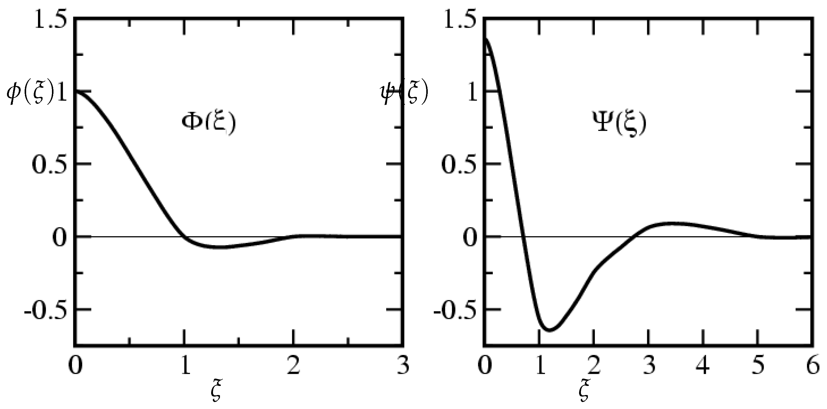
2. Wavelet Based Solution of PDEs
3. Volume Rendering in Compression Domain
4. Numerical Results and Discussion
Available Volume Rendering Software
5. The Proposed Rendering Techniques
5.1. Direct Summation of Wavelets
5.2. Ray Casting
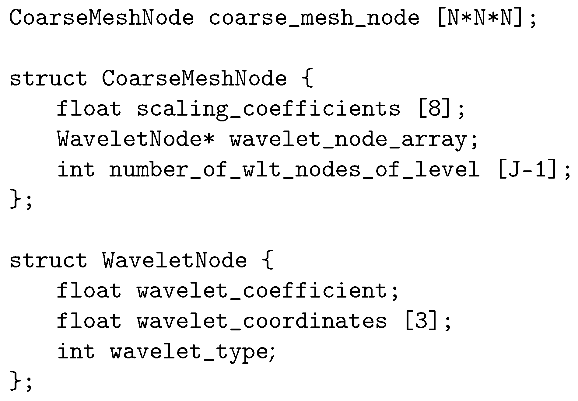
5.3. Data Structure
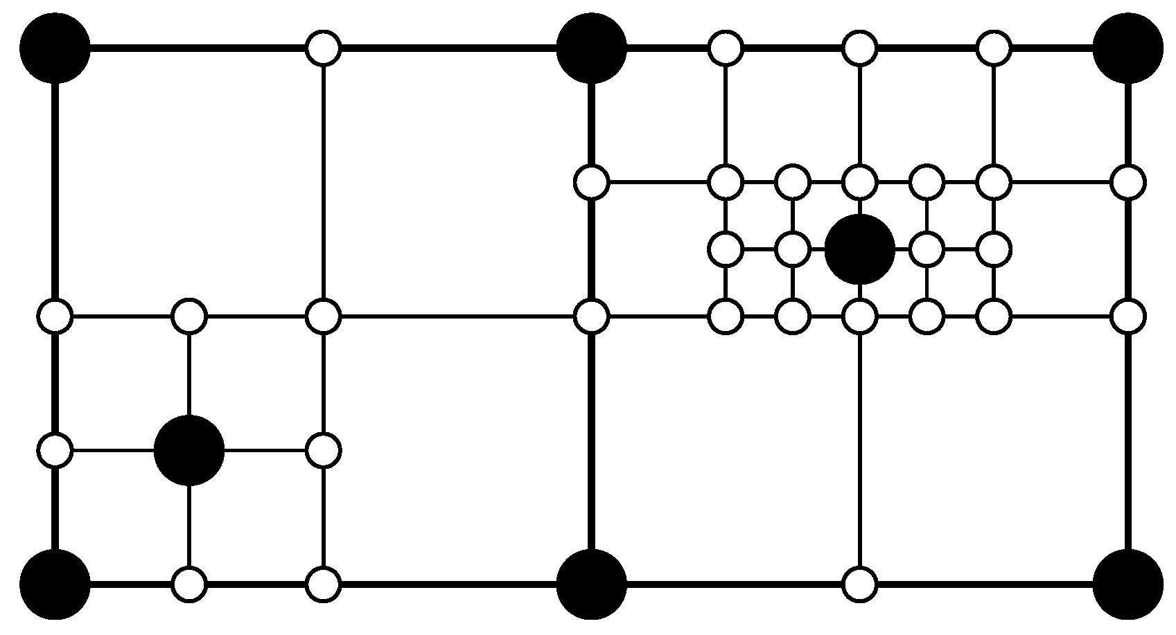
5.4. Adaptive Wavelet Grid and AMR
5.5. Completing Wavelet Based Grid to AMR
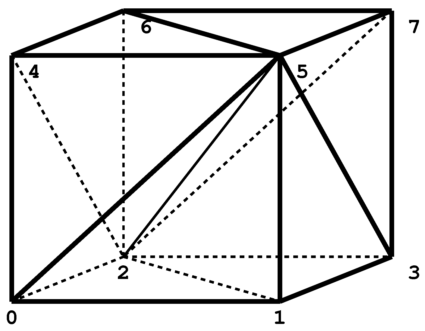
5.6. AMR Volume Rendering
6. Results
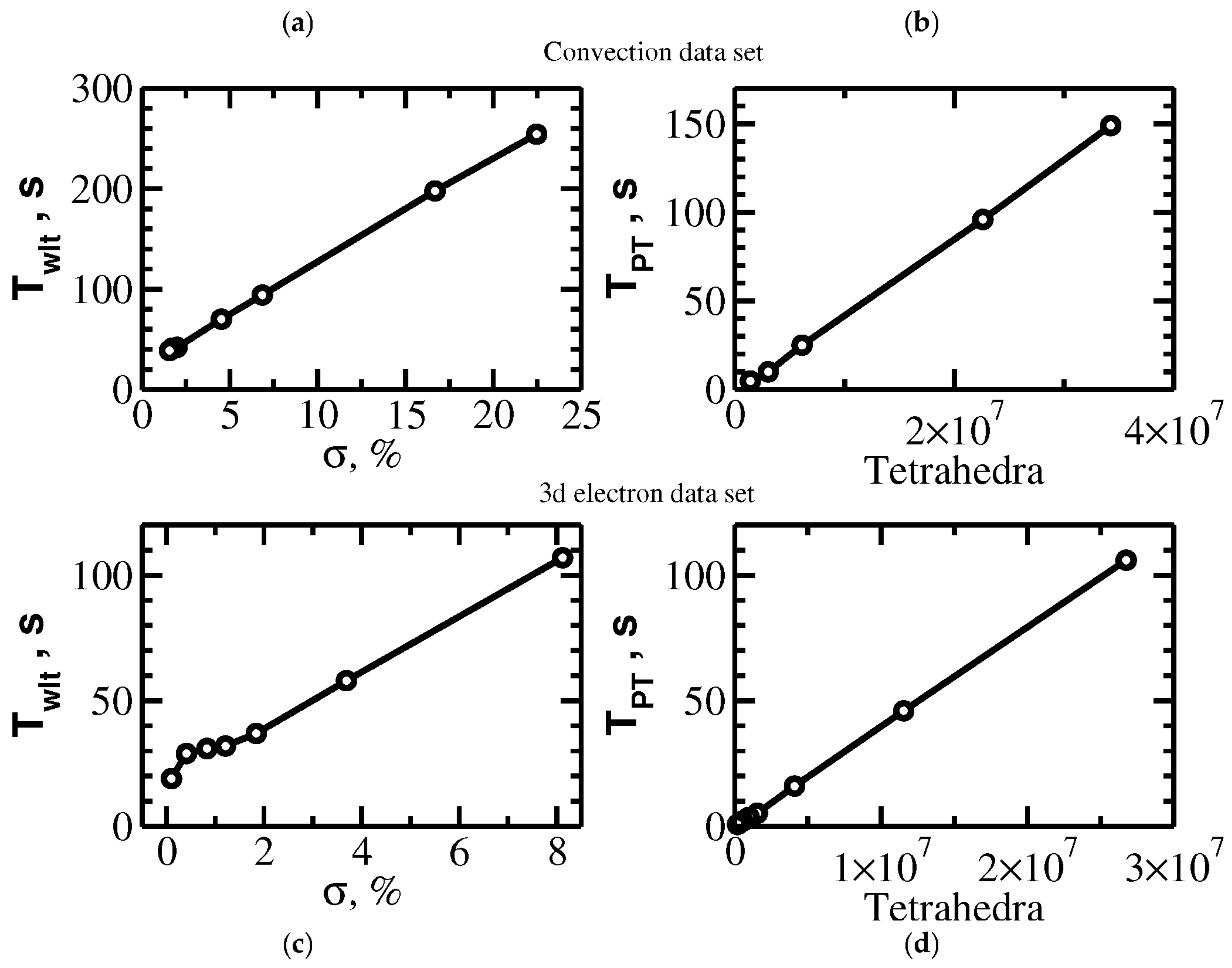
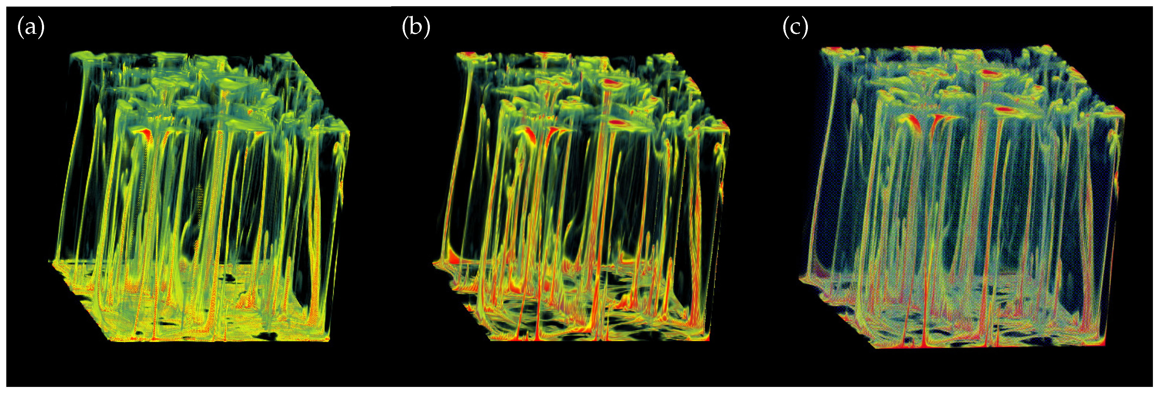
6.1. Convection Data Sets
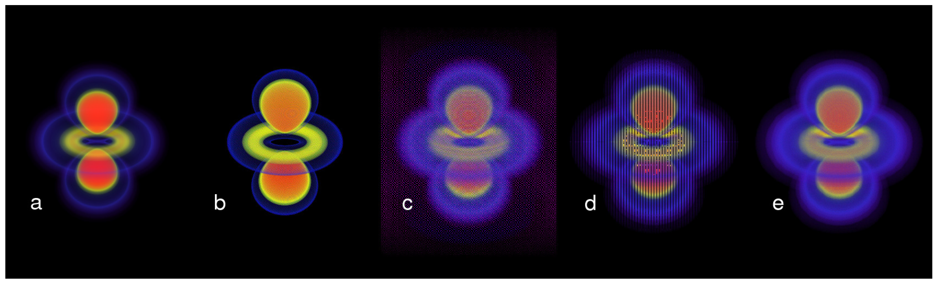
6.2. Hydrogen 3D Orbital Data Sets
6.3. Rendering Results
7. Conclusions and Future Work
Author Contributions
Funding
Conflicts of Interest
Abbreviations
| AMR | adaptive mesh refinement |
| PDE | partial differential equation |
| VTK | Visualization Toolkit |
| VT VOXEL | orthogonal parallelepiped-type VTK cell |
| VTK TETRA | tetrahedra type VTK cell |
References
- Vasilyev, O.V.; Bowman, C. Second generation wavelet collocation method for the solution of partial differential equations. J. Comput. Phys. 2000, 165, 660–693. [Google Scholar] [CrossRef] [Green Version]
- Cruz, P.; Mendes, A.; Magalhães, F.D. Wavelet-based adaptive grid method for the resolution of nonlinear PDEs. AIChE J. 2002, 48, 774–785. [Google Scholar] [CrossRef]
- Schneider, K.; Vasilyev, O.V. Wavelet Methods in Computational Fluid Dynamics. Ann. Rev. Fluid Mech. 2010, 42, 473–503. [Google Scholar] [CrossRef] [Green Version]
- Nejadmalayeri, A.; Vezolainen, A.; Brown-Dymkoski, E.; Vasilyev, O.V. Parallel adaptive wavelet collocation method for PDEs. J. Comput. Phys. 2015, 298, 237–253. [Google Scholar] [CrossRef] [Green Version]
- Berger, M.J.; Oliger, J. Adaptive mesh refinement for hyperbolic partial differential equations. J. Comput. Phys. 1984, 53, 484–512. [Google Scholar] [CrossRef]
- Berger, M.; Colella, P. Local adaptive mesh refinement for shock hydrodynamics. J. Comput. Phys. 1989, 82, 64–84. [Google Scholar] [CrossRef] [Green Version]
- Linde, T.J.; Weirs, V.G.; Plewa, T. Adaptive Mesh Refinement—Theory and Applications; Springer: Berlin/Heidelberg, Germany, 2008. [Google Scholar]
- Vasilyev, O.V.; Yuen, D.A.; Paolucci, S. The Solution of PDEs Using Wavelets. Comput. Phys. 1997, 11, 429–435. [Google Scholar] [CrossRef]
- Kiris, C.C.; Barad, M.F.; Housman, J.A.; Sozer, E.; Brehm, C.; Moini-Yekta, S. The LAVA Computational Fluid Dynamics Solver. In Proceedings of the 52nd Aerospace Sciences Meeting, National Harbor, MD, USA, 13–17 January 2014. [Google Scholar] [CrossRef]
- Adams, M.; Colella, P.; Graves, D.; Johansen, H.; Keen, N.; Ligocki, T.J.; Martin, D.; McCorquodale, P.; Modiano, D.; Schwartz, P.O.; et al. Chombo Software Package for AMR Applications—Design Document; Applied Numerical Algorithms Group Computational Research Division Lawrence Berkeley National Laboratory: Berkeley, CA, USA, 2015.
- Rossinelli, D.; Hejazialhosseini, B.; Spampinato, D.G.; Koumoutsakos, P. Multicore/multi-GPU accelerated simulations of multiphase compressible flows using wavelet adapted grids. SIAM J. Sci. Comput. 2011, 33, 512–540. [Google Scholar] [CrossRef]
- Kevlahan, N.K.R.; Dubos, T. WAVETRISK-1.0: An adaptive wavelet hydrostatic dynamical core. Geosci. Model Dev. 2019, 12, 4901–4921. [Google Scholar] [CrossRef] [Green Version]
- Paolucci, S.; Zikoski, Z.J.; Wirasaet, D. WAMR: An adaptive wavelet method for the simulation of compressible reacting flow. Part I. Accuracy and efficiency of algorithm. J. Comput. Phys. 2014, 272, 814–841. [Google Scholar] [CrossRef]
- Paolucci, S.; Zikoski, Z.J.; Grenga, T. WAMR: An adaptive wavelet method for the simulation of compressible reacting flow. Part II. The parallel algorithm. J. Comput. Phys. 2014, 272, 842–864. [Google Scholar] [CrossRef]
- Schroeder, W.; Martin, K.; Lorensen, B. The Visualization Toolkit, 4th ed.; Kitware: Clifton Park, NY, USA, 2006. [Google Scholar]
- Ayachit, U. The ParaView Guide: A Parallel Visualization Application; Kitware: Vienna, Austria, 2015. [Google Scholar]
- Childs, H.; Brugger, E.; Whitlock, B.; Meredith, J.; Ahern, S.; Pugmire, D.; Biagas, K.; Miller, M.; Harrison, C.; Weber, G.H.; et al. VisIt: An End-User Tool For Visualizing and Analyzing Very Large Data. In High Performance Visualization–Enabling Extreme-Scale Scientific Insight; CRC Press: Boca Raton, FL, USA, 2012; pp. 357–372. [Google Scholar] [CrossRef]
- Ligocki, T. Implementing a Visualization Tool for Adaptive Mesh Refinement Data using VTK. In Proceedings of the Visualization Development Environments, Princeton, NJ, USA, 27–28 April 2000. [Google Scholar]
- Wald, I.; Brownlee, C.; Usher, W.; Knoll, A. CPU Volume Rendering of Adaptive Mesh Refinement Data. In Proceedings of the SIGGRAPH Asia 2017 Symposium on Visualization, Los Angeles, CA, USA, 30 July–3 August 2017; ACM: New York, NY, USA, 2017; pp. 9:1–9:8. [Google Scholar] [CrossRef]
- Ma, K.L.; Crockett, T. A scalable parallel cell-projection volume rendering algorithm for three-dimensional unstructured data. In Proceedings of the IEEE Symposium on Parallel Rendering (PRS’97), Phoenix, AZ, USA, 20–21 October 1997; pp. 95–104. [Google Scholar] [CrossRef]
- Kaehler, R.; Hege, H.C. Texture-based volume rendering of adaptive mesh refinement data. Vis. Comput. 2002, 18, 481–492. [Google Scholar] [CrossRef] [Green Version]
- Kaehler, R.; Wise, J.; Abel, T.; Hege, H.C. GPU-Assisted Raycasting for Cosmological Adaptive Mesh Refinement Simulations; Volume Graphics; Machiraju, R., Moeller, T., Eds.; The Eurographics Association: Munich, Germany, 2006. [Google Scholar] [CrossRef]
- Kaehler, R.; Abel, T. Single-pass GPU-raycasting for structured adaptive mesh refinement data. In Proceedings of the SPIE, Burlingame, CA, USA, 3–7 February 2013; Wong, P.C., Kao, D.L., Hao, M.C., Chen, C., Healey, C.G., Eds.; SPIE: Bellingham, CA, USA, 2013. [Google Scholar] [CrossRef] [Green Version]
- Leaf, N.; Vishwanath, V.; Insley, J.; Hereld, M.; Papka, M.E.; Ma, K.L. Efficient parallel volume rendering of large-scale adaptive mesh refinement data. In Proceedings of the 2013 IEEE Symposium on Large-Scale Data Analysis and Visualization (LDAV), Atlanta, GA, USA, 13–14 October 2013; pp. 35–42. [Google Scholar] [CrossRef]
- Weber, G.H.; Childs, H.; Meredith, J.S. Efficient parallel extraction of crack-free isosurfaces from adaptive mesh refinement (AMR) data. In Proceedings of the IEEE Symposium on Large Data Analysis and Visualization (LDAV), Seattle, WA, USA, 14–15 October 2012; pp. 31–38. [Google Scholar] [CrossRef] [Green Version]
- Sweldens, W. The lifting scheme: A construction of second generation wavelets. SIAM J. Math. Anal. 1998, 29, 511–546. [Google Scholar] [CrossRef] [Green Version]
- Vasilyev, O.V. Solving multi-dimensional evolution problems with localized structures using second generation wavelets. Int. J. Comput. Fluid Dyn. 2003, 17, 151–168. [Google Scholar] [CrossRef]
- Vasilyev, O.V.; Kevlahan, N.K.R. An adaptive multilevel wavelet collocation method for elliptic problems. J. Comput. Phys. 2005, 206, 412–431. [Google Scholar] [CrossRef] [Green Version]
- Muraki, S. Approximation and rendering of volume data using wavelet transforms. In Proceedings of the Visualization ’92, Boston, MA, USA, 19–23 October 1992; pp. 21–28. [Google Scholar] [CrossRef]
- Lippert, L.; Gross, M.; Kurmann, C. Compression Domain Volume Rendering for Distributed Environments. Comput. Graph. Forum 1997, 16, C95–C107. [Google Scholar] [CrossRef] [Green Version]
- Westermann, R. A Multiresolution Framework for Volume Rendering. In Proceedings of the 1994 Symposium on Volume Visualization, Washington, DC, USA, 17–18 October 1994; Association for Computing Machinery: New York, NY, USA, 1994; pp. 51–58. [Google Scholar]
- Guthe, S.; Wand, M.; Gonser, J.; Strasser, W. Interactive rendering of large volume data sets. IEEE Vis. 2002, 2002, 53–60. [Google Scholar]
- Welsh, T.; Mueller, K. A Frequency-Sensitive Point Hierarchy for Images and Volumes. IEEE Vis. 2003, 2003, 425–432. [Google Scholar] [CrossRef]
- Lippert, L.; Gross, M.H. Fast Wavelet Based Volume Rendering by Accumulation of Transparent Texture Maps. In Computer Graphics Forum; Blackwell Science Ltd.: Edinburgh, UK, 1995. [Google Scholar] [CrossRef]
- Gross, M.; Lippert, L.; Dittrich, R.; Häring, S. Two methods for wavelet-based volume rendering. Comput. Graph. 1997, 21, 237–252. [Google Scholar] [CrossRef] [Green Version]
- Bajaj, C.; Ihm, I.; Koo, G.B.; Park, S. Parallel Ray Casting of Visible Human on Distributed Memory Architectures; Gröller, E., Löffelmann, H., Ribarsky, W., Eds.; Springer: Vienna, Austria, 1999; pp. 269–276. [Google Scholar]
- Nguyen, K.G.; Saupe, D. Rapid High Quality Compression of Volume Data for Visualization. In Computer Graphics Forum; Blackwell Science Ltd.: Edinburgh, UK, 2001; Volume 20. [Google Scholar]
- Lippert, L.; Gross, M.H. Ray-Tracing of Multiresolution B-Spline Volumes; Technical Report 239; Computer Science Department, ETH: Zürich, Switzerland, 1996. [Google Scholar]
- Yu, H.; Chang, E.C.; Huang, Z.; Zheng, Z. Fast Rendering of Foveated Volume in the Wavelet Domain. In Proceedings of the IEEE Visualization 2004, Austin, TX, USA, 10–15 October 2004. [Google Scholar] [CrossRef]
- Freitag, L.; Loy, R. Adaptive, Multiresolution Visualization of Large Data Sets using a Distributed Memory Octree. In Proceedings of the SC ’99: Proceedings of the 1999 ACM/IEEE Conference on Supercomputing, Portland, OR, USA, 13–19 November 1999; p. 60. [Google Scholar]
- Kreylos, O.; Weber, G.H.; Wes, E.; John, B.; Shalf, M.; Hamann, B.; Joy, K.I. Remote Interactive Direct Volume Rendering of AMR Data; Technical report; Lawrence Berkeley National Laboratory: Berkeley, CA, USA, 2002. [Google Scholar]
- Weber, G.H.; Kreylos, O.; Ligocki, T.J.; Shalf, J.; Hagen, H.; Hamann, B.; Joy, K.I.; Ma, K.L. High-Quality Volume Rendering of Adaptive Mesh Refinement Data; Vision, Modeling and Visualization; Aka GmbH: Augsburg, Germany, 2001; pp. 121–128. [Google Scholar]
- Lacroute, P.; Levoy, M. Fast Volume Rendering Using a Shear-Warp Factorization of the Viewing Transformation. In Proceedings of the SIGGRAPH ’94, Orlando, FL, USA, 24–29 July 1994; Association for Computing Machinery: New York, NY, USA, 1994; pp. 451–458. [Google Scholar]
- Lacroute, P. The VolPack Volume Rendering Library; Stanford University: Stanford, CA, USA, 1995. [Google Scholar]
- Schroeder, W.; Martin, K.; Lorensen, W. The design and implementation of an object-oriented toolkit for 3D graphics and visualization. In Proceedings of the Seventh Annual IEEE Visualization ’96, San Francisco, CA, USA, 27 October–1 November 1996; pp. 93–100. [Google Scholar] [CrossRef]
- Schroeder, W.; Geveci, B.; Malaterre, M. Compatible triangulations of spatial decompositions. IEEE Vis. 2004, 2004, 211–217. [Google Scholar] [CrossRef]
- Amira-User’s Guide and Reference Manual; Zuse Institute Berlin (ZIB) and Indeed-Visual Concepts GmbH: Berlin, Germany, 2001.


| Data Set | , % | , % | F, M | , M | |||||
|---|---|---|---|---|---|---|---|---|---|
| 0.0005 | 22.5 | 87.1 | 101 | 2199 | 254 | - | - | - | |
| 0.001 | 16.7 | 74.9 | 75 | 1847 | 198 | - | - | - | |
| 0.005 | 6.85 | 39.9 | 31 | 915 | 94 | 149 | - | - | |
| Convection | 0.01 | 4.51 | 27.3 | 21 | 607 | 70 | 96 | - | - |
| 0.05 | 1.99 | 8.15 | 9.0 | 167 | 42 | 25 | 100 | - | |
| 0.1 | 1.72 | 3.82 | 7.8 | 83 | 41 | 10 | 58 | - | |
| 0.5 | 1.56 | 1.55 | 7.1 | 38 | 39 | 4.8 | 43 | 97 | |
| 8.12 | 28.8 | 37 | 706 | 107 | 106 | - | - | ||
| 3.69 | 12.9 | 17 | 306 | 58 | 46 | - | - | ||
| 1.84 | 4.71 | 8.3 | 109 | 37 | 16 | 54 | 7400 | ||
| 3D electron | 1.21 | 1.65 | 5.5 | 41 | 32 | 5.2 | 35 | 210 | |
| 0.83 | 1.04 | 3.8 | 26 | 31 | 3.6 | 29 | 78 | ||
| 0.41 | 0.60 | 1.9 | 15 | 29 | 2.1 | 25 | 57 | ||
| 0.10 | 0.22 | 0.5 | 5 | 19 | 0.7 | 22 | 38 |
Publisher’s Note: MDPI stays neutral with regard to jurisdictional claims in published maps and institutional affiliations. |
© 2022 by the authors. Licensee MDPI, Basel, Switzerland. This article is an open access article distributed under the terms and conditions of the Creative Commons Attribution (CC BY) license (https://creativecommons.org/licenses/by/4.0/).
Share and Cite
Vezolainen, A.V.; Erlebacher, G.; Vasilyev, O.V.; Yuen, D.A. Volumetric Rendering on Wavelet-Based Adaptive Grid. Fluids 2022, 7, 245. https://doi.org/10.3390/fluids7070245
Vezolainen AV, Erlebacher G, Vasilyev OV, Yuen DA. Volumetric Rendering on Wavelet-Based Adaptive Grid. Fluids. 2022; 7(7):245. https://doi.org/10.3390/fluids7070245
Chicago/Turabian StyleVezolainen, Alexei V., Gordon Erlebacher, Oleg V. Vasilyev, and David A. Yuen. 2022. "Volumetric Rendering on Wavelet-Based Adaptive Grid" Fluids 7, no. 7: 245. https://doi.org/10.3390/fluids7070245
APA StyleVezolainen, A. V., Erlebacher, G., Vasilyev, O. V., & Yuen, D. A. (2022). Volumetric Rendering on Wavelet-Based Adaptive Grid. Fluids, 7(7), 245. https://doi.org/10.3390/fluids7070245