A Wavelet-Based Adaptive Finite Element Method for the Stokes Problems

Abstract

In this work, we present the mathematical formulation of the new adaptive multiresolution method for the Stokes problems of highly viscous materials arising in computational geodynamics. The method is based on particle-in-cell approach—the Stokes system is solved on a static Eulerian finite element grid and material properties are carried in space by Lagrangian material points. The Eulerian grid is adapted using the wavelet-based adaptation algorithm. Both bilinear (${\mathrm{Q}}_1{\mathrm{P}}_0$, ${\mathrm{Q}}_1{\mathrm{Q}}_1$) and biquadratic (${\mathrm{Q}}_2{\mathrm{P}}_{-1}$) mixed approximations for the Stokes system are supported. The proposed method is illustrated for a number of linear and nonlinear two-dimensional benchmark problems of geophysical relevance. The results of the adaptive numerical simulations using the proposed method are in an excellent agreement with those obtained on non-adaptive grids and with analytical solutions, while computational requirements are few orders of magnitude less compared to the non-adaptive simulations in terms of both time and memory usage.

1. Introduction

Practical problems of computational geodynamics require high-resolution numerical models. Computational requirements of such models can be very high, and thus powerful supercomputers are employed routinely nowadays. However, to utilize these machines more efficiently and to be able to model truly challenging problems like global mantle convection at numerical resolutions resolving $1\mathrm{km}$ scales, new advanced computational methods are needed (e.g., [1,2,3].

In this work we present the novel adaptive multiresolution method for mechanical Stokes problems arising in computational geodynamics. The Stokes system of equations is solved on a static Eulerian finite element grid which is adapted in space based on chosen adaptation criterion (viscosity field, strain rate field, etc.), and material properties and history are carried by Lagrangian particles. Fully automatic grid adaptation is implemented using an original algorithm based on wavelet analysis [4,5,6,7,8]. The adaptation is supported for both bilinear (${\mathrm{Q}}_1{\mathrm{P}}_0$, ${\mathrm{Q}}_1{\mathrm{Q}}_1$) and biquadratic (${\mathrm{Q}}_2{\mathrm{P}}_{-1}$) finite element grids.

The work is divided into 2 parts. In the first part (Section 2, Section 3, Section 4, Section 5, Section 6 and Section 7), the mathematical formulation and implementation details of the method are given. In the second part (Section 8), we discuss the results of some numerical benchmarks.

2. Governing Equations

We are interested in very slow deformations of highly viscous materials, typical for mantle convection problems. In problems of geophysical relevance due to drastically different convection and viscous time scales, both material properties and scalar quantities are advected as described in Section 4, while viscous forces are assumed to be in equilibrium. In this case all inertial forces can be neglected and such quasi-static deformation process can be described as an evolution through a succession of equilibria:

$$\frac{\partial {\sigma }_{ij}}{\partial x_j}+\rho f_i=0$$

(1)

where ${\sigma }_{ij}$ is the total stress tensor component, $f_i$ is the external force per unit mass vector component, $x_j$ indicates the spatial coordinate and $\rho$ is the density.

The medium is assumed to be incompressible. Thus, Equation (1) is solved subject to incompressibility condition:

$${\dot{\epsilon }}_{ii}=0$$

(2)

where ${\dot{\epsilon }}_{ij}$ is the strain rate tensor component defined as:

$${\dot{\epsilon }}_{ij}=\frac{1}{2}\left(\frac{\partial v_i}{\partial x_j}+\frac{\partial v_j}{\partial x_i}\right)$$

(3)

where $v_i$ and $v_j$ indicate the velocities.

The relation between dynamic ($\sigma$) and kinematic ($\dot{\epsilon }$) quantities is given by rheological constitutive equation. For viscous incompressible medium it is expressed as (e.g., [9]):

$${\sigma }_{ij}=-p{\delta }_{ij}+2\eta {\dot{\epsilon }}_{ij}$$

(4)

where p is the pressure, ${\delta }_{ij}$ is the Kronecker delta, $\eta$ is the viscosity.

Equations (1)–(4) form the incompressible Stokes system. Even though the adaptive finite element method is generalizable to three dimensions, in this work both the method formulation and its applications are limited to two-dimensional problems. Thus we assume strain tensor components ${\epsilon }_{zz},{\epsilon }_{xz},{\epsilon }_{zx},{\epsilon }_{yz},{\epsilon }_{zy}$ to be equal 0 (plane strain assumption) and the system we solve takes the form:

$$\begin{array}{cc}\hfill 2\frac{\partial }{\partial x}\left(\eta \frac{\partial v_x}{\partial x}\right)+\frac{\partial }{\partial y}\left(\eta \frac{\partial v_x}{\partial y}+\eta \frac{\partial v_y}{\partial x}\right)-\frac{\partial p}{\partial x}& =-\rho f_x\hfill \\ \hfill 2\frac{\partial }{\partial y}\left(\eta \frac{\partial v_y}{\partial y}\right)+\frac{\partial }{\partial x}\left(\eta \frac{\partial v_y}{\partial x}+\eta \frac{\partial v_x}{\partial y}\right)-\frac{\partial p}{\partial y}& =-\rho f_y\hfill \\ \hfill \frac{\partial v_x}{\partial x}+\frac{\partial v_y}{\partial y}& =0\hfill \end{array}$$

(5)

Viscoplastic rheology is implemented by using a non-linear effective viscosity in Equation (5). A material deforms viscously when stresses fall below its yield strength ${\sigma }_{\mathrm{yield}}$, but plastic deformations occur as soon as ${\sigma }_{\mathrm{yield}}$ is reached, and the effective viscosity is adjusted to ensure material strength ${\sigma }_{\mathrm{yield}}$ is never exceeded (e.g., [10,11,12]):

$${\eta }_{\mathrm{eff}}=min\{{\eta }_{\mathrm{creep}},\frac{{\sigma }_{\mathrm{yield}}}{2{\dot{\epsilon }}_{II}}\}$$

(6)

Here ${\eta }_{\mathrm{creep}}$ is the creep viscosity, which is a function of strain rate and other material parameters in general cases, and is a constant if viscous deformations are linear (e.g., [9]), ${\sigma }_{\mathrm{yield}}$ is the yield strength of a material and ${\dot{\epsilon }}_{II}$ is the second invariant of the strain rate tensor defined as:

$${\dot{\epsilon }}_{II}=\sqrt{\frac{1}{2}{\dot{\epsilon }}_{ij}{\dot{\epsilon }}_{ij}}$$

(7)

The yield strength ${\sigma }_{\mathrm{yield}}$ is calculated according to the Drucker-Prager plasticity model, which in general form is expressed as (e.g., [13]):

$${\sigma }_{\mathrm{yield}}=\alpha p+\beta$$

(8)

where p is the pressure, $\alpha$ and $\beta$ are material parameters. The following relationships for $\alpha$ and $\beta$ are used [14]:

$$\alpha =sin\left(\varphi \right),\beta =ccos\left(\varphi \right)$$

(9)

where c and $\varphi$ are cohesion and friction angle of a material respectively.

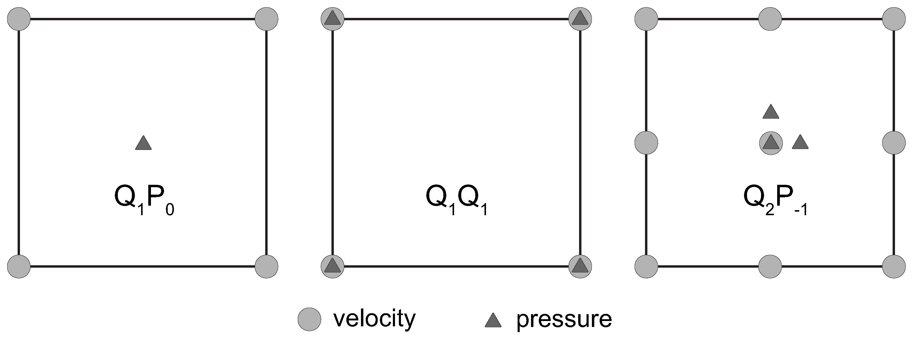
3. Finite Element Discretization of the Stokes System

The Stokes system of Equation (5) is solved on an Eulerian grid using Galerkin mixed finite element discretization technique. In this way velocities and pressure are approximated as:

$$\begin{array}{c}{v}_x(x,y)\simeq {\displaystyle \sum _{i=1}^n}{N}_i(x,y)v_{xi}{v}_y(x,y)\simeq {\displaystyle \sum _{i=1}^n}{N}_i(x,y)v_{yi}\\ p(x,y)\simeq {\displaystyle \sum _{i=1}^m}{M}_i(x,y)p_i\end{array}$$

(10)

where n and m are numbers of velocity and pressure nodes, $N_i$ and $M_i$ are locally defined basis functions, $v_{xi}$, $v_{yi}$ and $p_i$ are nodal values of velocities and pressure which have to be found.

In this work we employ 3 different quadrilateral element types (i.e., combinations of basis sets $\left\{N_i\right\}$ and $\left\{M_i\right\}$): bilinear velocity—constant discontinuous pressure ${\mathrm{Q}}_1{\mathrm{P}}_0$, bilinear velocity—bilinear continuous pressure ${\mathrm{Q}}_1{\mathrm{Q}}_1$ with stabilization, biquadratic velocity—linear discontinuous pressure ${\mathrm{Q}}_2{\mathrm{P}}_{-1}$ (Figure 1; for exact expressions of basis functions see e.g., [15]). Probably the most popular in the community is the ${\mathrm{Q}}_1{\mathrm{P}}_0$ element, primary due to its low computational costs. However, this approximation is unstable as it does not satisfy inf-sup condition and so can lead to highly inaccurate results under some circumstances [16,17]. The ${\mathrm{Q}}_1{\mathrm{Q}}_1$ approximation is also inherently unstable, but it can be stabilized by very efficient and simple to implement method proposed recently [18,19]. Finally, the ${\mathrm{Q}}_2{\mathrm{P}}_{-1}$ element is stable and known to be robust [17], but associated computational cost is significantly higher compared to bilinear approximations ${\mathrm{Q}}_1{\mathrm{P}}_0$ or ${\mathrm{Q}}_1{\mathrm{Q}}_1$.

Substitution of Equation (10) into Equation (5) and application of Galerkin discretization procedure yield the Stokes system of equations in the matrix form (e.g., [20]:

$$\left[\begin{array}{cc}\mathbf{A}& \mathbf{Q}\\ {\mathbf{Q}}^{\mathrm{T}}& \mathbf{0}\end{array}\right]\left[\begin{array}{c}\mathbf{v}\\ \mathbf{p}\end{array}\right]=\left[\begin{array}{c}\mathbf{F}\\ \mathbf{0}\end{array}\right]$$

(11)

where stiffness matrix $\mathbf{A}$, gradient operator matrix $\mathbf{Q}$, right hand side vector $\mathbf{F}$ and vectors of unknowns $\mathbf{v}$ and $\mathbf{p}$ are:

$$\begin{array}{c}\mathbf{A}={\int }_{\Omega }{\mathbf{B}}^{\mathrm{T}}\mathbf{D}\mathbf{B}dxdy\mathbf{Q}=-{\int }_{\Omega }{\mathbf{K}}^{\mathrm{T}}\mathbf{H}dxdy\mathbf{F}={\int }_{\Omega }{\mathbf{R}}^{\mathrm{T}}dxdy\\ \mathbf{v}={\left[\begin{array}{c}{v}_{x1}{v}_{y1}{v}_{x2}{v}_{y2}\dots v_{xn}{v}_{yn}\end{array}\right]}^{\mathrm{T}}\mathbf{p}={\left[\begin{array}{c}{p}_1{p}_2\dots p_m\end{array}\right]}^{\mathrm{T}}\end{array}$$

(12)

Here vectors and matrices $\mathbf{B}$, $\mathbf{D}$, $\mathbf{K}$, $\mathbf{H}$ and $\mathbf{R}$ are:

$$\begin{array}{cccc}\hfill \mathbf{B}& =\left[\begin{array}{c}\Lambda N_1\Lambda N_2\dots \Lambda N_n\end{array}\right]\hfill & \hfill & \mathrm{where}\Lambda =\left[\begin{array}{cc}\frac{\partial }{\partial x}& 0\\ 0& \frac{\partial }{\partial y}\\ \frac{\partial }{\partial y}& \frac{\partial }{\partial x}\end{array}\right]\hfill \\ \hfill \mathbf{D}& =\eta \left[\begin{array}{ccc}2& 0& 0\\ 0& 2& 0\\ 0& 0& 1\end{array}\right]\hfill \\ \hfill \mathbf{K}& =\left[\begin{array}{c}\nabla N_1\nabla N_2\dots \nabla N_n\end{array}\right]\hfill & \hfill & \mathrm{where}\nabla =\left[\begin{array}{cc}\frac{\partial }{\partial x}& \frac{\partial }{\partial y}\end{array}\right]\hfill \\ \hfill \mathbf{H}& =\left[\begin{array}{c}{M}_1{M}_2\dots M_m\end{array}\right]\hfill \\ \hfill \mathbf{R}& =\left[\begin{array}{c}{N}_{1}X{N}_{2}X\dots N_{n}X\end{array}\right]\hfill & \hfill & \mathrm{where}X=\rho \left[\begin{array}{cc}{f}_x& f_y\end{array}\right]\hfill \end{array}$$

(13)

In case of ${\mathrm{Q}}_1{\mathrm{Q}}_1$ approximation, the system (11) has to be further modified to include stabilization matrix [18,19]:

$$\left[\begin{array}{cc}\mathbf{A}& \mathbf{Q}\\ {\mathbf{Q}}^{\mathrm{T}}& -\mathbf{V}\end{array}\right]\left[\begin{array}{c}\mathbf{v}\\ \mathbf{p}\end{array}\right]=\left[\begin{array}{c}\mathbf{F}\\ \mathbf{0}\end{array}\right]$$

(14)

where stabilization matrix $\mathbf{V}$ is:

$$\mathbf{V}=\frac{1}{\eta }{\int }_{\Omega }{\overline{\mathbf{H}}}^{\mathrm{T}}\overline{\mathbf{H}}dxdy$$

(15)

where vector $\overline{\mathbf{H}}$ is:

$$\overline{\mathbf{H}}=\left[\begin{array}{c}{M}_1-\frac{1}{4}{M}_2-\frac{1}{4}\dots M_m-\frac{1}{4}\end{array}\right]$$

(16)

Since basis functions $N_i$ and $M_i$ are locally defined, matrices $\mathbf{A}$, $\mathbf{Q}$ and $\mathbf{V}$ in Equations (11) and (14) are sparse and in practise are built by assembling contributions from individual elements.

The problem (11) is solved by augmented Lagrangian iterative method (e.g., [21,22]). First, the system (11) is amended by addition of the term $-\frac{1}{k}\mathbf{M}$ to the both sides of the second equation, and velocity Schur complement is computed as:

$$\widehat{\mathbf{A}}=\mathbf{A}+k\mathbf{Q}{\mathbf{M}}^{-1}{\mathbf{Q}}^{\mathrm{T}}$$

(17)

where k is the penalty parameter and $\mathbf{M}$ is the mass matrix:

$$\mathbf{M}={\int }_{\Omega }{\mathbf{H}}^{\mathrm{T}}\mathbf{H}dxdy$$

(18)

Schur complement $\widehat{\mathbf{A}}$ is then factorized and the iterative scheme is employed until sufficient level of incompressibility defined by ${ϵ}_{\mathrm{inc}}$ is reached. The matrix $\widehat{\mathbf{A}}$ is symmetric positive definite, and so the Cholesky factorization is employed:

$$\begin{array}{cc}\hfill & \widehat{\mathbf{A}}\to \mathbf{L}{\mathbf{L}}^{\mathrm{T}}\hfill \\ \hfill & \mathrm{DO}\hfill \\ \hfill & {\mathbf{v}}^{\mathrm{i}}={\mathbf{L}}^{-\mathrm{T}}\left({\mathbf{L}}^{-1}(\mathbf{F}-\mathbf{Q}{\mathbf{p}}^{\mathrm{i}})\right)\hfill \\ \hfill & {\mathbf{d}}^{\mathrm{i}}={\mathbf{M}}^{-1}{\mathbf{Q}}^{\mathrm{T}}{\mathbf{v}}^{\mathrm{i}}\hfill \\ \hfill & {\mathbf{p}}^{\mathrm{i}+1}={\mathbf{p}}^{\mathrm{i}}+k{\mathbf{d}}^{\mathrm{i}}\hfill \\ \hfill & \mathrm{i}=\mathrm{i}+1\hfill \\ \hfill & \mathrm{UNTIL}{\parallel {\mathbf{d}}^{\mathrm{i}}\parallel }_{\infty }>{ϵ}_{\mathrm{inc}}\hfill \end{array}$$

(19)

Augmented Lagrangian method is very efficient, but it implies inversion of the mass matrix $\mathbf{M}$. It is easy to compute the inverse ${\mathbf{M}}^{-1}$ when pressure approximation is discontinuous, which is true when ${\mathrm{Q}}_1{\mathrm{P}}_0$ or ${\mathrm{Q}}_2{\mathrm{P}}_{-1}$ elements are employed. However, in case of ${\mathrm{Q}}_1{\mathrm{Q}}_1$ element we deal with the system (14), and it is not feasible to apply the method (19) since pressure approximation is continuous. The system (14) is symmetric but always indefinite, and in the current work we solve it at once using LDL factorization. Representing the problem (14) as $\mathbf{S}\mathbf{x}=\mathbf{b}$ this implies:

$$\begin{array}{cc}\hfill & \mathbf{S}\to \mathbf{L}\mathbf{D}{\mathbf{L}}^{\mathrm{T}}\hfill \\ \hfill & \mathbf{x}={\mathbf{L}}^{-\mathrm{T}}\left({\mathbf{D}}^{-1}\left({\mathbf{L}}^{-1}\mathbf{b}\right)\right)\hfill \end{array}$$

(20)

Both methods (19) and (20) rely on direct matrix factorization. Strong advantage of direct factorization methods is the possibility to use them as black boxes for ill-conditioned systems which typically arise in geodynamic models. On the other hand, CPU and memory requirements of direct methods are high and thus application of such methods to significantly large systems of linear equations is difficult and iterative schemes are used instead [23,24]. However, as will be shown in this work, introduction of dynamic mesh adaptation reduces the number of unknowns and thus the cost of factorization dramatically, and makes it possible to use direct methods for models of quite high efficient numerical resolution even in case of expensive ${\mathrm{Q}}_2{\mathrm{P}}_{-1}$ mixed approximation.

Non-linearities arising in case of plastic yielding are treated using the method of successive substitutions (also known as Picard’s method, see e.g., [25]). At first, effective viscosities are calculated with some initial velocity and pressure fields. The stiffness matrix $\mathbf{A}$ is built then, and depending on element type the Stokes problem is solved either by Equations (19) or (20). Then effective viscosities are recalculated using the new solution and matrix $\mathbf{A}$ is rebuilt. These steps are repeated until the maximum number of non-linear iterations is passed or convergence criterion is reached:

$$\frac{{\parallel {\mathbf{v}}_{\mathrm{nl}}^{\mathrm{i}}-{\mathbf{v}}_{\mathrm{nl}}^{\mathrm{i}-1}\parallel }_2}{{\parallel {\mathbf{v}}_{\mathrm{nl}}^{\mathrm{i}}\parallel }_2}<{ϵ}_{\mathrm{nl}}$$

(21)

where ${\mathbf{v}}_{\mathrm{nl}}^{\mathrm{i}}$ is the velocity solution obtained at non-linear iteration $\mathrm{i}$ and ${ϵ}_{\mathrm{nl}}$ is the non-linear tolerance.

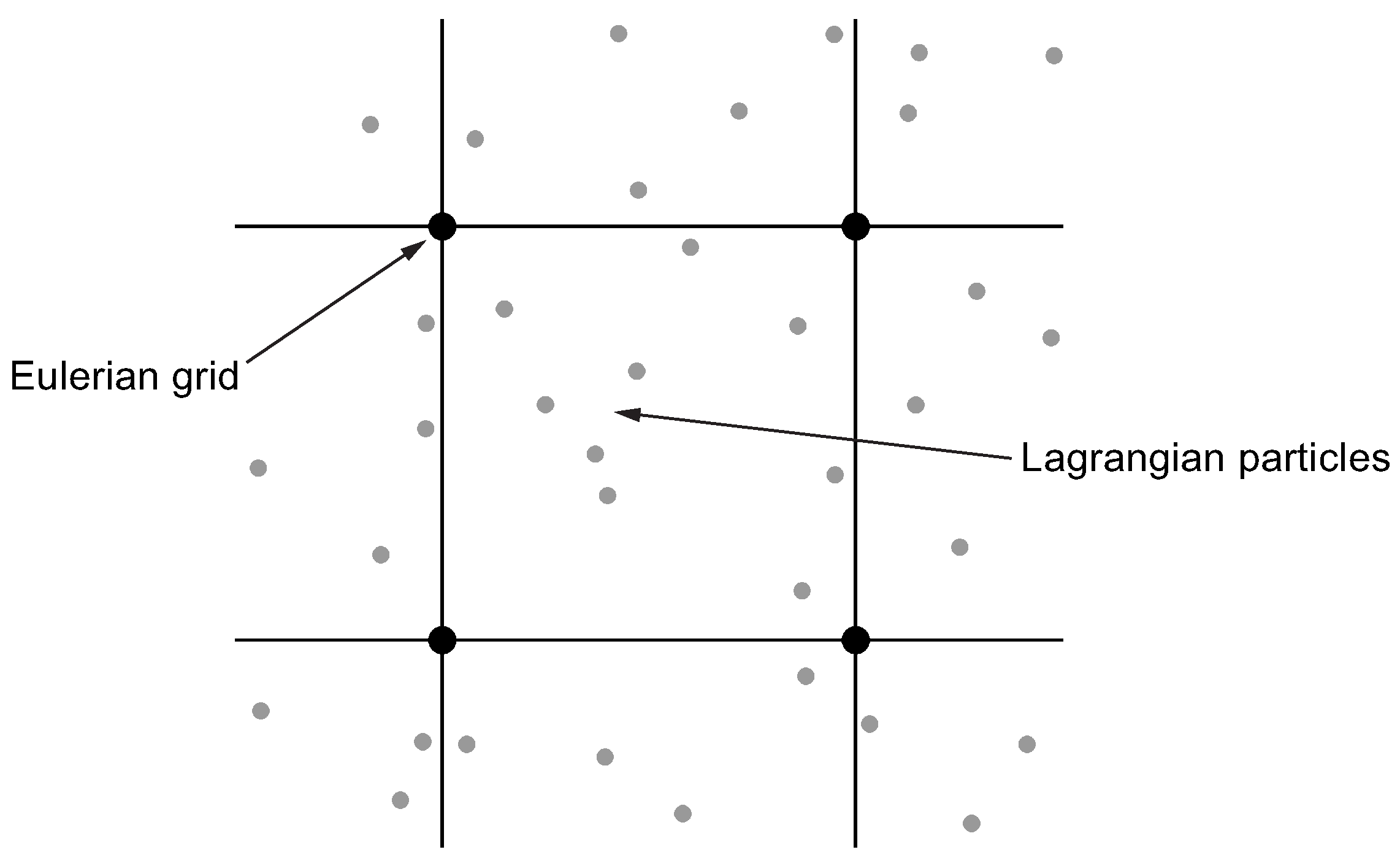
4. Particle-In-Cell Simulation Methodology

The material properties and history are carried by Lagrangian material points, which are advected using the solution of the Stokes system obtained on a static grid (Figure 2). Such a combination of Lagrangian and Eulerian frames is known as the particle-in-cell method and is widely used in computational geodynamics (e.g., [26,27,28]). The method allows accurate tracking of material interfaces, and can be used for modeling of very large deformations without necessity to perform re-gridding, which is required in case of alternative Arbitrary Lagrangian-Eulerian approach (e.g., [10]).

The PIC simulation algorithm can be described as a succession of the following actions performed at each time step:

• Interpolation of physical properties from Lagrangian particles to Eulerian grid.
• Assemblage of the Stokes system using interpolated physical properties.
• Solution of the system on an Eulerian grid (see Section 3).
• Interpolation of computed velocities to Lagrangian particles positions.
• Particles advection using the interpolated velocities.

Time integration is performed by the first-order forward Euler scheme. Thus each particle p is advected as:

$${\mathbf{x}}_p(t+\Delta t)={\mathbf{x}}_p\left(t\right)+{\mathbf{v}}_p\left(t\right)\Delta t$$

(22)

where ${\mathbf{x}}_p$ is the particle’s coordinate vector, ${\mathbf{v}}_p$ is the interpolated velocity vector of a particle, and $\Delta t$ is the time step calculated based on a given Courant number.

The accuracy of Equation (22) is normally enough. However, if necessary, higher order integration methods can be used, for example the Runge-Kutta of fourth-order (e.g., [29]).

Initially, the Lagrangian particles are distributed randomly, but with uniform density. The initial uniform density, however, is not usually well preserved as simulation proceeds. The problem can be solved using the approach based on discrete Voronoi tessellation [30,31], which is described as follows. First, each element of computational Eulerian grid is discretized by a structured lattice. The lattice is then divided into sub-domains (discrete Voronoi cells) in such a way that each sub-domain consists of all lattice cells closer to an associated particle than to any other particle residing in the element. The accuracy of such an approximate Voronoi diagram depends on a resolution of the lattice (Figure 3). Then, areas of discrete Voronoi cells are computed and compared to empirical thresholds $A{V}_{min}$ and $A{V}_{max}$. Physically, the cell areas are considered as weights of associated Lagrangian particles, so particles whose weights are below $A{V}_{min}$ are eliminated, and those with weights above $A{V}_{max}$ are cloned. When cloning is performed, the new particle is added to the centroid of corresponding Voronoi cell (Figure 4). The centroid coordinate vector ${\mathbf{x}}_{\mathrm{centroid}}$ is computed as:

$${\mathbf{x}}_{\mathrm{centroid}}=\frac{{\sum }_{i=1}^{n_{\mathrm{cl}}}{\mathbf{x}}_{\mathrm{cl}}^i}{n_{\mathrm{cl}}}$$

(23)

where ${\mathbf{x}}_{\mathrm{cl}}^i$ and $n_{\mathrm{cl}}$ are, respectively, the coordinate vectors and the total number of the lattice cells constituting the Voronoi cell.

Usually, some trial experiments are required to find appropriate values for $A{V}_{min}$ and $A{V}_{max}$. Once these values are estimated, the algorithm works very efficiently to maintain uniform density of Lagrangian particle field.

5. Wavelet-Based Grid Adaptation

In this section we describe the implementation of the grid adaptation methodology based on wavelet analysis. First, the linear interpolating wavelet transform will be introduced. Next, the wavelet-based grid adaptation algorithm will be presented.

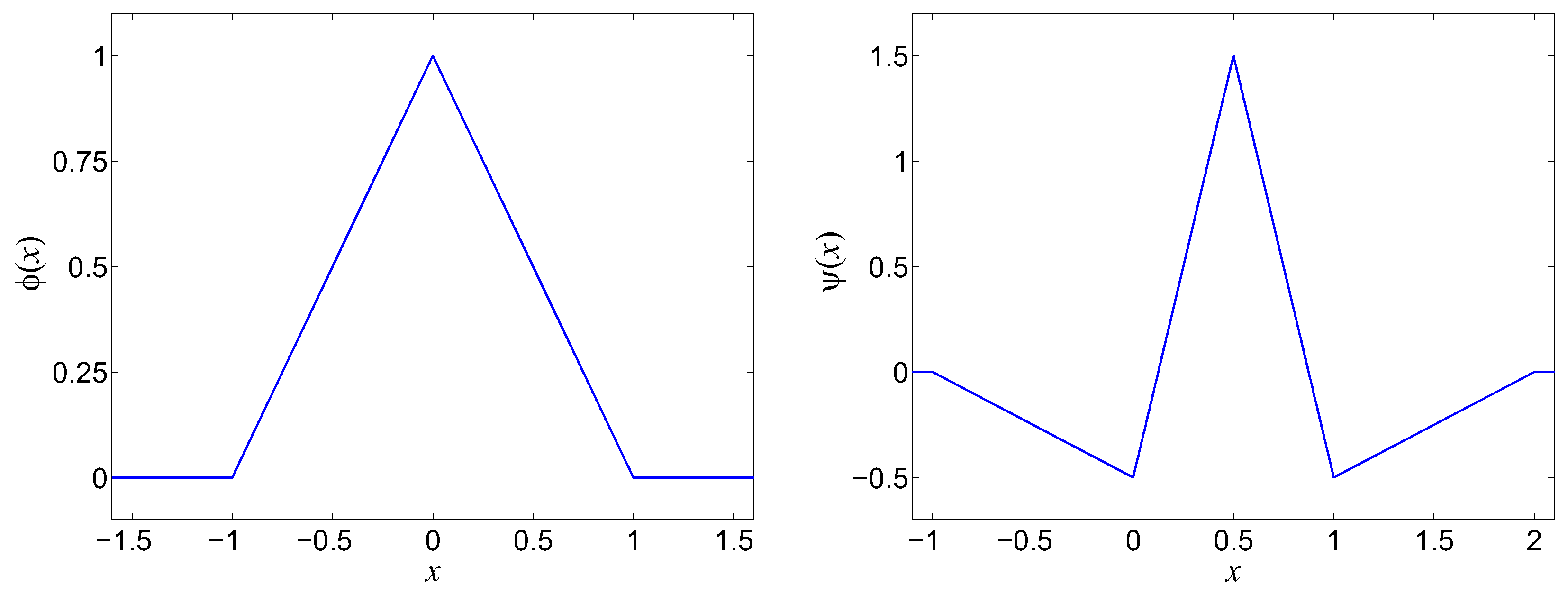
5.1. Linear Interpolating Wavelet Transform

In general, the wavelet transform is a very efficient methodology to construct the multilevel decomposition of some given function. Considering one dimensional case, a function $f\left(x\right)$ defined at $m{2}^{(n-1)}+1$ points (m is arbitrary integer number) can be decomposed to n levels from $J=n-1$ (finest) to 0 (coarsest) in such a way that at each level the function is approximated as $f^j$ (e.g., [32]):

$$f^J\left(x\right)=\underset{f^j}{\underbrace{\underset{f^1}{\underbrace{f^0+w^0}}+\cdots +w^{j-1}}}+\cdots +w^{J-1}$$

(24)

where $f^0$ is the function approximation at the coarsest level, and each $w^j$ represents a difference between approximations at levels j and $j+1$:

$$\begin{array}{cc}\hfill f^0& =\sum _{k\in {\mathcal{K}}^0}{c}_k^0{\varphi }_k^0\left(x\right)\hfill \\ \hfill w^j& =\sum _{l\in {\mathcal{L}}^j}{d}_l^j{\psi }_l^j\left(x\right)\hfill \end{array}$$

(25)

Further substitution of Equation (25) into Equation (24) yields:

$$f^J\left(x\right)=\sum _{k\in {\mathcal{K}}^0}{c}_k^0{\varphi }_k^0\left(x\right)+\sum _{j=0}^{J-1}\sum _{l\in {\mathcal{L}}^j}{d}_l^j{\psi }_l^j\left(x\right)$$

(26)

where ${\mathcal{K}}^0$ and ${\mathcal{L}}^j$ are index sets, ${\varphi }_k^j\left(x\right)$ and ${\psi }_l^j\left(x\right)$ are scaling functions and wavelets respectively, and $c_k^j$ and $d_l^j$ are scaling function and wavelet coefficients respectively. This is the purpose of the forward wavelet transform to determine $c_k^j$ and $d_l^j$.

Once the decomposition (26) is obtained, we can analyze wavelet coefficients $d_l^j$, which indicate differences between function approximations at neighbor levels, and leave only significant $d_l^j$ with absolute values above some prescribed threshold $\epsilon$. This way the compact representation $f_{⩾}^J\left(x\right)$ of the original function $f\left(x\right)$ is constructed:

$$f^J\left(x\right)=\underset{\mathrm{compact}\mathrm{representation},f_{⩾}^J\left(x\right)}{\underbrace{\sum _{k\in {\mathcal{K}}^0}{c}_k^0{\varphi }_k^0\left(x\right)+{\displaystyle \sum _{j=0}^{J-1}}\sum _{\begin{array}{c}l\in {\mathcal{L}}^j\\ |d_l^j|⩾\epsilon \end{array}}{d}_l^j{\psi }_l^j\left(x\right)}}+\underset{\mathrm{insignificant},f_{<}^J\left(x\right)}{\underbrace{{\displaystyle \sum _{j=0}^{J-1}}\sum _{\begin{array}{c}l\in {\mathcal{L}}^j\\ |d_l^j|<\epsilon \end{array}}{d}_l^j{\psi }_l^j\left(x\right)}}$$

(27)

Scaling functions ${\varphi }_k^j\left(x\right)$ and wavelets ${\psi }_l^j\left(x\right)$ are spawned by dilations and translations of father wavelet $\varphi \left(x\right)$ and mother wavelet $\psi \left(x\right)$ respectively:

$$\begin{array}{cc}\hfill {\varphi }_k^j\left(x\right)& =\varphi (2^{j}x-k)\hfill \\ \hfill {\psi }_k^j\left(x\right)& =\psi (2^{j}x-k)\hfill \end{array}$$

(28)

We use the linear interpolating transform in this work. This dictates the following expressions for $\varphi \left(x\right)$ and $\psi \left(x\right)$ (see Figure 5 for the corresponding plots):

$$\begin{array}{cc}\hfill \varphi \left(x\right)& =max\{0,1-|x\left|\right\}\hfill \\ \hfill \psi \left(x\right)& =2\varphi (2x-1)-\frac{1}{2}\varphi \left(x\right)-\frac{1}{2}\varphi (x-1)\hfill \end{array}$$

(29)

Different techniques to perform forward wavelet transform exist. The very suitable one to work with interpolating wavelets is the lifting scheme [33], which is employed in this work. In case of linear interpolating $\varphi \left(x\right)$ and $\psi \left(x\right)$, as in Equation (29), the lifted transform from level $j+1$ to level j is (e.g., [34]):

$$\begin{array}{cc}\hfill d_k^j& =\frac{1}{2}(c_{2k+1}^{j+1}-\frac{1}{2}(c_{2k}^{j+1}+c_{2k+2}^{j+1}))\hfill \\ \hfill c_k^j& =c_{2k}^{j+1}+\frac{1}{2}(d_{k-1}^j+d_k^j)\hfill \end{array}$$

(30)

The scheme (30) is applied sequentially starting from the finest level and proceeding to the coarsest one. This produces values for $c_k^j$ and $d_l^j$ at all resolution levels which can be analyzed then in accordance with Equation (27).

As an example consider the linear interpolating wavelet transform of the Gaussian function $f\left(x\right)=e^{-\frac{{(x-0.5)}^2}{{(1/64)}^2}}$ with further analysis for insignificant $d_l^j$ coefficients shown on Figure 6. Scaling function coefficients $c_k^0$ represent the coarsest resolution level, and levels $1\dots 5$ are represented by wavelet coefficients $d_l^j,j=0\dots 4$ respectively. Note how the Gaussian curve is captured by significant $d_l^j$ coefficients and how its approximation is sequentially refined at each level.

In two dimensional case, the 1D forward transform has to be performed in each dimension sequentially. Thus, given a function $f(x,y)$, the scheme (30) is applied first to x- and then to y-slices. The example of a two-dimensional function is considered in the next section.

5.2. Grid Adaptation Algorithm

The linear interpolating forward transform, described in the Section 5.1, can be applied to analyze a function representing some physical field of interest (viscosity $\eta$, density $\rho$, second strain rate invariant ${\dot{\epsilon }}_{II}$, etc.). The result of such an analysis can be used then as a guidance to build a multilevel computational grid. To facilitate the process, the nodes of computational grid are associated with scaling function $c_k^0$ and wavelet coefficients $d_l^j$. Based on these ideas, the wavelet-based grid adaptation algorithm proceeds as follows (see publications [4] and [6] for further details):

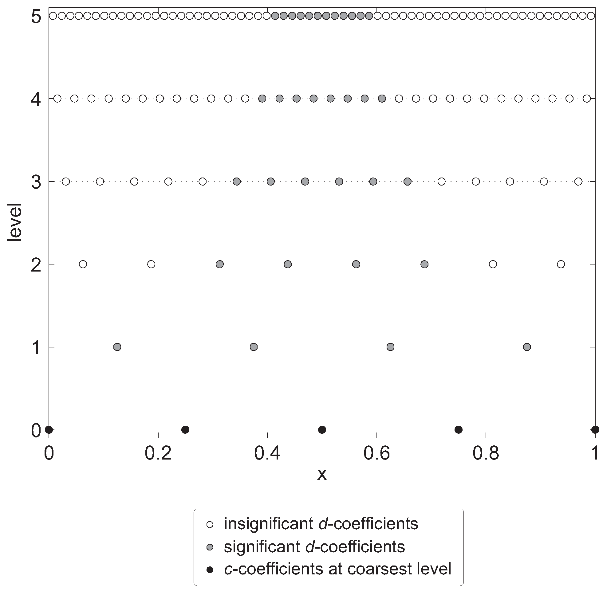
• Perform the forward wavelet transform of a physical field which is considered as an adaptation criterion and get all $c_k^0$ and $d_l^j$ coefficients. If a physical property field is defined on Lagrangian particles, the interpolation from particles to grid nodes is performed first.
• Analyze wavelet coefficients $d_l^j$ at all levels and create a mask $\mathcal{M}$ containing grid nodes associated with significant $d_l^j$.
• Include into the mask $\mathcal{M}$ all grid nodes from the coarsest level, i.e. associated with coefficients $c_k^0$.
• Extend the mask $\mathcal{M}$ with grid nodes associated with adjacent to significant $d_l^j$. This is to ensure that the mask $\mathcal{M}$ includes all nodes whose coefficients can potentially become significant at the next simulation time step.
• Apply recursively the reconstruction check procedure to the mask $\mathcal{M}$. This is to guarantee that all wavelet coefficients $d_l^j$ necessary to perform the forward transform at the next time step will be available.
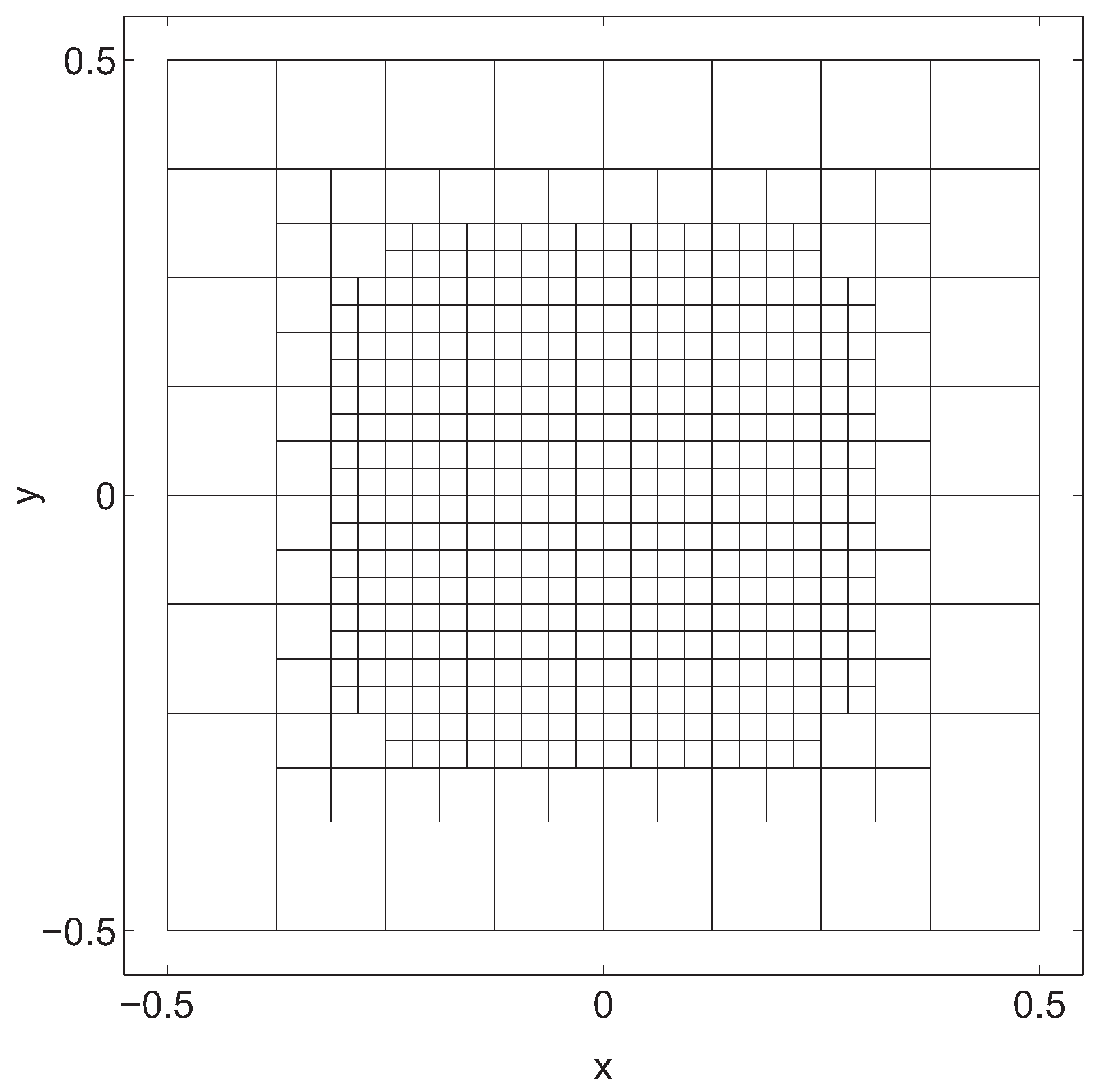
• Using the adapted mask $\mathcal{M}$, construct a new multilevel finite element grid.

As an example, consider the linear interpolating wavelet transform of the 2-D Gaussian function $f(x,y)=e^{-\frac{x^2+y^2}{2{\left(0.07\right)}^2}}$. The mask $\mathcal{M}$ shown on Figure 7a was obtained by applying the two dimensional forward transform and including grid nodes associated with significant $d_l^j$ and all $c_k^0$ into $\mathcal{M}$.

Further, extending $\mathcal{M}$ with grid nodes associated with adjacent wavelet coefficients and applying the reconstruction check procedure, the complete adapted mask $\mathcal{M}$ becomes as shown on Figure 7b. Based on the mask, the multilevel computational grid is built (Figure 8, bilinear discretization is assumed), which is then used to assemble and solve the Stokes system of equations.

Normally, the new grid is constructed in this way at each simulation time step. Note that this does not impose any changes to the particle-in-cell simulation algorithm.

If necessary, several adaptation criteria can be used simultaneously. In such a case, each criterion is analyzed independently and the corresponding mask ${\mathcal{M}}_i$ is created. The nodewise OR combination of all ${\mathcal{M}}_i$ gives the common mask $\mathcal{M}$, which is then used for multilevel grid construction.

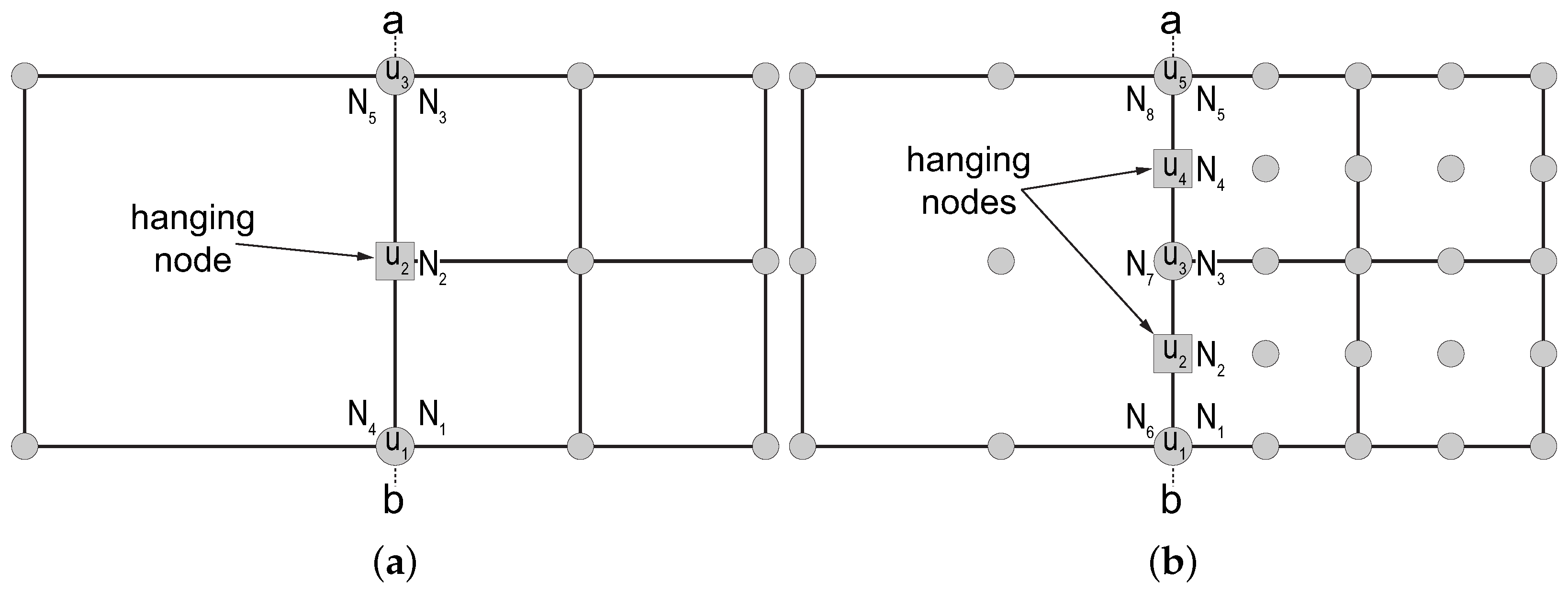
6. Dealing with Hanging Nodes

A multilevel grid, like one shown on Figure 8, is inherently non-conforming due to the presence of hanging nodes on boundaries between unequal grid levels. In order to obtain correct results on such a non-conforming grid, procedures of assemblage and solution of a corresponding system of equations have to be modified.

Bilinear ($Q_1$) and biquadratic ($Q_2$) basis functions, employed in this work, impose an approximated function to be continues across the element edges. Examining in this way the typical segment of $Q_1$ multilevel grid shown on Figure 9a, the approximation for an unknown function u has to be continues across the edge $\mathbf{ab}$. This implies that for any point lying on the edge $\mathbf{ab}$ the following equality has to hold:

$$u_1{N}_1(x,y)+u_2{N}_2(x,y)+u_3{N}_3(x,y)=u_1{N}_4(x,y)+u_3{N}_5(x,y)$$

(31)

where $u_i$ are unknown nodal values of the function u, and $N_i$ are bilinear basis functions.

The degree of freedom corresponding to a hanging node has to be constrained to satisfy of the continuity requirement (31). Since bilinear approximation is considered, the constraint is expressed as:

$$u_2=\frac{1}{2}(u_1+u_3)$$

(32)

Generalizing, the relationship between unconstrained and constrained degrees of freedom defined on the edge $\mathbf{ab}$ can be expressed in the matrix form as:

$${\mathbf{u}}^{\mathbf{ab}}={\mathbf{M}}_{\mathbf{u}}^{\mathbf{ab}}{\tilde{\mathbf{u}}}^{\mathbf{ab}}$$

(33)

where ${\mathbf{u}}^{\mathbf{ab}}$ and ${\tilde{\mathbf{u}}}^{\mathbf{ab}}$ are unconstrained and constrained vectors of unknowns respectively, and ${\mathbf{M}}_{\mathbf{u}}^{\mathbf{ab}}$ is the transformation matrix:

$$\begin{array}{c}{\mathbf{u}}^{\mathbf{ab}}=\left[\begin{array}{c}{u}_1\\ u_2\\ u_3\end{array}\right]{\tilde{\mathbf{u}}}^{\mathbf{ab}}=\left[\begin{array}{c}{u}_1\\ u_3\end{array}\right]{\mathbf{M}}_{\mathbf{u}}^{\mathbf{ab}}=\left[\begin{array}{cc}1& 0\\ \frac{1}{2}& \frac{1}{2}\\ 0& 1\end{array}\right]\end{array}$$

(34)

In case of biquadratic basis functions, the similar to Equation (31) continuity requirement across the edge $\mathbf{ab}$ for the typical segment of $Q_2$ multilevel grid shown on Figure 9b is formulated as:

$$\begin{array}{c}{u}_1{N}_1(x,y)+u_2{N}_2(x,y)+u_3{N}_3(x,y)+u_4{N}_4(x,y)+\hspace{1em}\hfill \\ \hfill \hspace{1em}+u_5{N}_5(x,y)=u_1{N}_6(x,y)+u_3{N}_7(x,y)+u_5{N}_8(x,y)\end{array}$$

(35)

To satisfy the requirement (35), hanging degrees of freedom $u_2$ and $u_4$ have to be constrained by a second-order Lagrange polynomial constructed using values $u_1$, $u_3$ and $u_5$. Thus, the transformation between unconstrained and constrained vectors of unknowns can be expressed using the matrix relation (33), where ${\mathbf{u}}^{\mathbf{ab}}$ and ${\tilde{\mathbf{u}}}^{\mathbf{ab}}$ vectors and matrix ${\mathbf{M}}_{\mathbf{u}}^{\mathbf{ab}}$ are:

$$\begin{array}{c}{\mathbf{u}}^{\mathbf{ab}}=\left[\begin{array}{c}{u}_1\\ u_2\\ u_3\\ u_4\\ u_5\end{array}\right]{\tilde{\mathbf{u}}}^{\mathbf{ab}}=\left[\begin{array}{c}{u}_1\\ u_3\\ u_5\end{array}\right]{\mathbf{M}}_{\mathbf{u}}^{\mathbf{ab}}=\left[\begin{array}{ccc}1& 0& 0\\ \frac{3}{8}& \frac{6}{8}& -\frac{1}{8}\\ 0& 1& 0\\ -\frac{1}{8}& \frac{6}{8}& \frac{3}{8}\\ 0& 0& 1\end{array}\right]\end{array}$$

(36)

Apparently, the similar to (33) transformation between unconstrained and constrained degrees of freedom can be formulated for the whole system. Thereby, considering the Stokes problem on a multilevel grid, the velocity constraint relationship is expressed as:

$$\mathbf{v}={\mathbf{M}}_{\mathbf{v}}\tilde{\mathbf{v}}$$

(37)

where $\mathbf{v}$ and $\tilde{\mathbf{v}}$ are unconstrained and constrained velocity vectors respectively, and ${\mathbf{M}}_{\mathbf{v}}$ is the transformation matrix. Note that $\mathbf{v}$ and $\tilde{\mathbf{v}}$ contain both x- and y-velocities and so ${\mathbf{M}}_{\mathbf{v}}$ has to be constructed accordingly.

Thus, the Stokes system of equations, assembled on a multilevel grid, has to be solved subject to constraint defined by (37). Note that this is the case if ${\mathrm{Q}}_1{\mathrm{P}}_0$ or ${\mathrm{Q}}_2{\mathrm{P}}_{-1}$ elements are used, and element ${\mathrm{Q}}_1{\mathrm{Q}}_1$ requires additional constraint on pressure due to the continuity of pressure approximation (see below). To impose constraint (37) on the Stokes system, the assembled stiffness matrix $\mathbf{A}$, gradient operator matrix $\mathbf{Q}$ and right hand side vector $\mathbf{F}$ are modified as [35,36]:

$$\begin{array}{cc}\hfill \tilde{\mathbf{A}}& ={\mathbf{M}}_{\mathbf{v}}^{\mathrm{T}}\mathbf{A}{\mathbf{M}}_{\mathbf{v}}\hfill \\ \hfill \tilde{\mathbf{Q}}& ={\mathbf{M}}_{\mathbf{v}}^{\mathrm{T}}\mathbf{Q}\hfill \\ \hfill \tilde{\mathbf{F}}& ={\mathbf{M}}_{\mathbf{v}}^{\mathrm{T}}\mathbf{F}\hfill \end{array}$$

(38)

And then these modified matrices are used in the standard solution procedure. This way, the velocity Schur complement (17) is computed as:

$$\widehat{\tilde{\mathbf{A}}}=\tilde{\mathbf{A}}+k\tilde{\mathbf{Q}}{\mathbf{M}}^{-1}{\tilde{\mathbf{Q}}}^{\mathrm{T}}$$

(39)

and augmented Lagrangian iterative method (19) is applied:

$$\begin{array}{cc}\hfill & \widehat{\tilde{\mathbf{A}}}\to \tilde{\mathbf{L}}{\tilde{\mathbf{L}}}^{\mathrm{T}}\hfill \\ \hfill & \mathrm{DO}\hfill \\ \hfill & {\tilde{\mathbf{v}}}^{\mathrm{i}}={\tilde{\mathbf{L}}}^{-\mathrm{T}}\left({\tilde{\mathbf{L}}}^{-1}(\tilde{\mathbf{F}}-\tilde{\mathbf{Q}}{\mathbf{p}}^{\mathrm{i}})\right)\hfill \\ \hfill & {\mathbf{v}}^{\mathrm{i}}={\mathbf{M}}_{\mathbf{v}}{\tilde{\mathbf{v}}}^{\mathrm{i}}\hfill \\ \hfill & \cdots \hfill \end{array}$$

(40)

Note, however, that unconstrained velocity vector ${\mathbf{v}}^{\mathrm{i}}$ is restored once the constrained solution ${\tilde{\mathbf{v}}}^{\mathrm{i}}$ is obtained.

In case if ${\mathrm{Q}}_1{\mathrm{Q}}_1$ element is employed, the additional constraint on pressure degrees of freedom is required:

$$\mathbf{p}={\mathbf{M}}_{\mathbf{p}}\tilde{\mathbf{p}}$$

(41)

where $\mathbf{p}$ and $\tilde{\mathbf{p}}$ are unconstrained and constrained pressure vectors respectively, and ${\mathbf{M}}_{\mathbf{p}}$ is the transformation matrix defined in a similar way as ${\mathbf{M}}_{\mathbf{v}}$.

To impose both velocity (37) and pressure constraint (41) on the Stokes system, the stiffness matrix $\mathbf{A}$ and right hand side vector $\mathbf{F}$ are modified in the same way as in (38), but gradient operator matrix $\mathbf{Q}$ and stabilization matrix $\mathbf{V}$ (which is required for ${\mathrm{Q}}_1{\mathrm{Q}}_1$ element) are modified as:

$$\begin{array}{cc}\hfill \tilde{\mathbf{Q}}& ={\mathbf{M}}_{\mathbf{v}}^{\mathrm{T}}\mathbf{Q}{\mathbf{M}}_{\mathbf{p}}\hfill \\ \hfill \tilde{\mathbf{V}}& ={\mathbf{M}}_{\mathbf{p}}^{\mathrm{T}}\mathbf{V}{\mathbf{M}}_{\mathbf{p}}\hfill \end{array}$$

(42)

The modified matrices are used to assemble the system which is then solved using LDL factorization (20). After that, the unconstrained velocity $\mathbf{v}$ and pressure $\mathbf{p}$ vectors are restored from the obtained $\tilde{\mathbf{v}}$ and $\tilde{\mathbf{p}}$ using Equations (37) and (41) respectively.

7. Implementation Aspects

The numerical method described in this work is implemented in MATLAB programming language. To facilitate further development, the object-oriented programming capabilities introduced with MATLAB 2008a are extensively used. Input/output is performed using HDF5 data format, which makes possible to use external packages for postprocessing.

The Cholesky decomposition is performed using Cholmod solver [37], and for LDL factorization the MA57 solver is employed [38]. Both are distributed with MATLAB as external libraries, although up-to-date versions of both can be downloaded. The permutation to reduce fill-in is done using approximate minimum degree ordering method [39].

Where data structures permit, MATLAB Parallel Computing Toolbox is used for parallelization. This makes possible to run the code efficiently on modern multi-core architectures, as well as in distributed environments.

The code is available for download from http://sites.google.com/site/sdvigus/ (last accessed on 28 June 2022).

8. Numerical Benchmarks

In the second part of this work, the results of lateral viscosity variation, sinking block, brittle extension/compression and Rayleigh-Taylor instability benchmarks are presented and discussed. The list of the benchmark problems studied and the main aspects of the algorithm they test are summarized in

Table 1. Benchmark problems studied.

Section	Benchmark Problem	Main Aspects of the Algorithm Tested by the Benchmark Problem
Section 8.1	Lateral viscosity variation	Comparison with the analytical solution
Section 8.2	Sinking block	Ability to handle large $O\left({10}^7\right)$ viscosity contrasts
Section 8.3	Brittle extension/compression	Ability to capture and resolve spontaneously forming shear zones
Section 8.4	Incompressibility test	Influence of the artificial incompressibility
Section 8.5	Rayleigh-Taylor instability	Comparison with the analytical solution

. For each problem we compare performance and accuracy of adaptive and non-adaptive schemes, and evaluate applicability of bilinear (${\mathrm{Q}}_1{\mathrm{P}}_0$, ${\mathrm{Q}}_1{\mathrm{Q}}_1$) and biquadratic (${\mathrm{Q}}_2{\mathrm{P}}_{-1}$) mixed approximations in different conditions. All numerical experiments were performed using MATLAB R2009b.

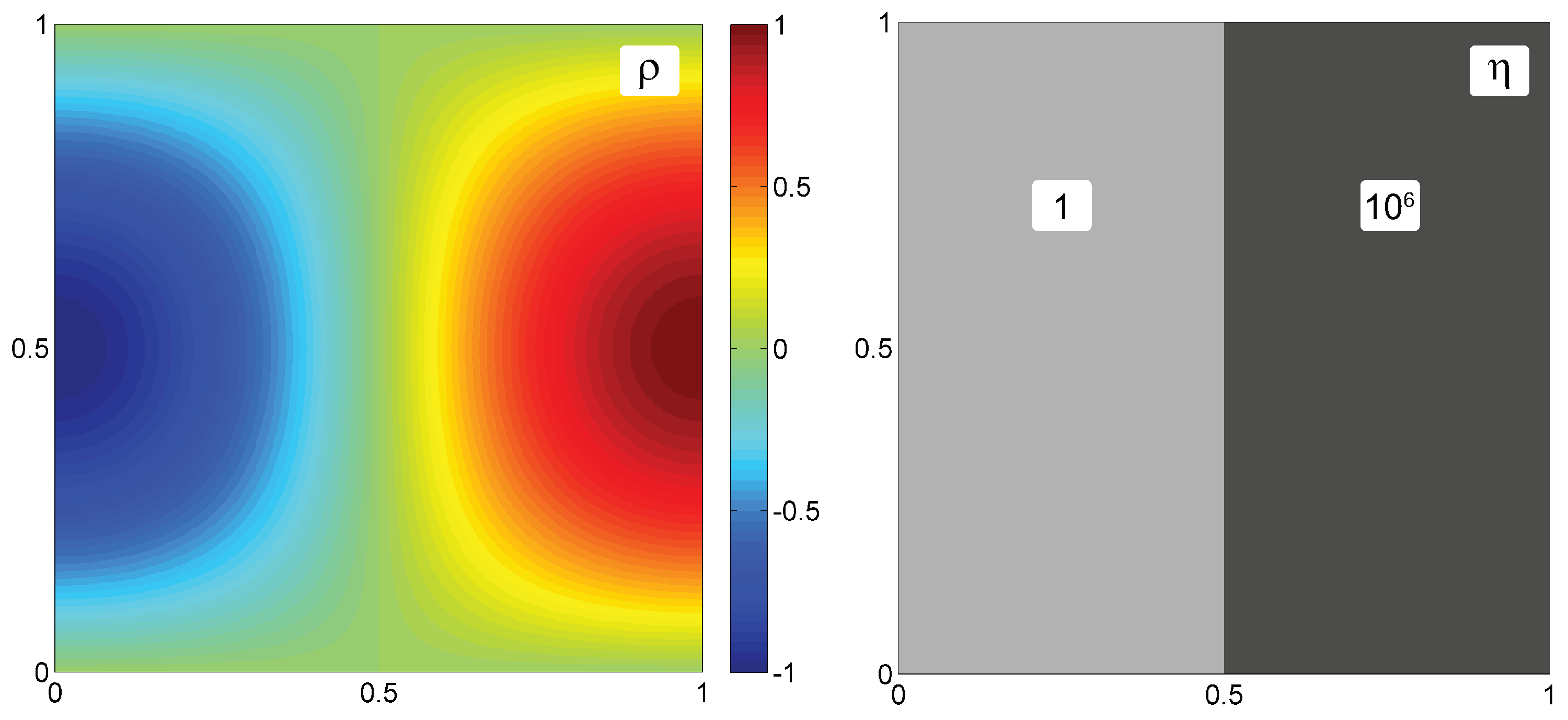
8.1. Lateral Viscosity Variation Benchmark

This is the sharp viscosity variation benchmark which is often referred to as SolCx (e.g., [24,40]. The fully developed analytical solution exists, and thus the convergence of the proposed adaptive numerical method and correctness of the implementation can be evaluated.

8.1.1. Setup and Parameters

The model domain is defined as $1.0\times 1.0$ box with free slip boundary conditions on all sides. The fluid flow is driven by density variation imposed by applying external force X as:

$$X=\rho (x,y){\left[\begin{array}{c}{f}_x\\ f_y\end{array}\right]}^{\mathrm{T}}\mathrm{where}\begin{array}{cc}\hfill & \rho (x,y)=sin\left(\pi y\right)cos\left(\pi x\right)\hfill \\ \hfill & f_x=0,f_y=1\hfill \end{array}$$

(43)

The sharp lateral viscosity variation is defined as:

$$\eta (x,y)=\left\{\begin{array}{cc}1,\hfill & \mathrm{if}0⩽x⩽0.5\hfill \\ {10}^6,\hfill & \mathrm{if}0.5<x⩽1\hfill \end{array}\right.$$

(44)

The plots showing initial density and viscosity profiles are provided on Figure 10.

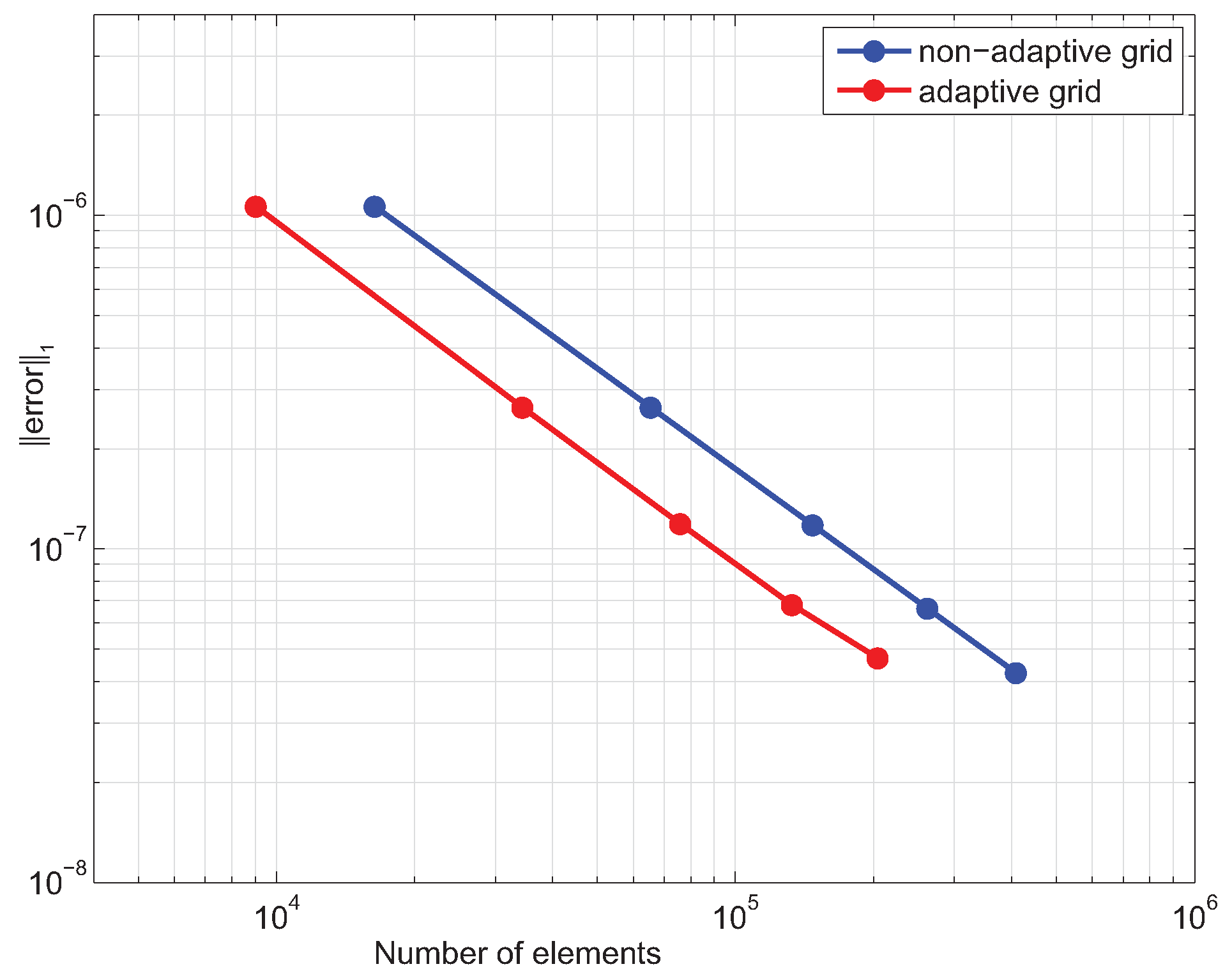
8.1.2. Convergence Test

The series of numerical experiments were performed on adaptive and non-adaptive ${\mathrm{Q}}_1{\mathrm{Q}}_1$-based grids of $128\times 128$, $256\times 256$, $384\times 384$, $512\times 512$ and $640\times 640$ efficient numerical resolutions. In case of adaptive grid, the $v_x$- and $v_y$-velocity fields served as adaptation criteria with a threshold $\epsilon ={10}^{-5}$. Thus, the wavelet-based adaptation was performed independently for each of velocity fields, and the results were combined to form a common adapted mask.

The normalized error between numerical and analytical [41] solutions was computed as:

$${\parallel error\parallel }_1=\sum _{i=1}^N\left(\right|{\overline{v}}_{xi}^{\mathrm{an}}-{\overline{v}}_{xi}^{\mathrm{num}}|+|{\overline{v}}_{yi}^{\mathrm{an}}-{\overline{v}}_{yi}^{\mathrm{num}}\left|\right)V_i$$

(45)

where N is the total number of elements, ${\overline{v}}_{xi}^{\mathrm{an}}$, ${\overline{v}}_{xi}^{\mathrm{num}}$, ${\overline{v}}_{yi}^{\mathrm{an}}$ and ${\overline{v}}_{yi}^{\mathrm{num}}$ are arithmetic means of analytical and numerical $v_x$- and $v_y$-velocities of i-element, $V_i$ is i-element volume.

Dependence of the normalized error on the number of elements for both adaptive and non-adaptive cases are shown in Figure 11. As it is clearly seen from the plots, both adaptive and non-adaptive methods converge with the same rate, but the convergence curve for the adaptive method is lower. Thus, the adaptive approach has a clear advantage—the higher accuracy for the same number of elements.

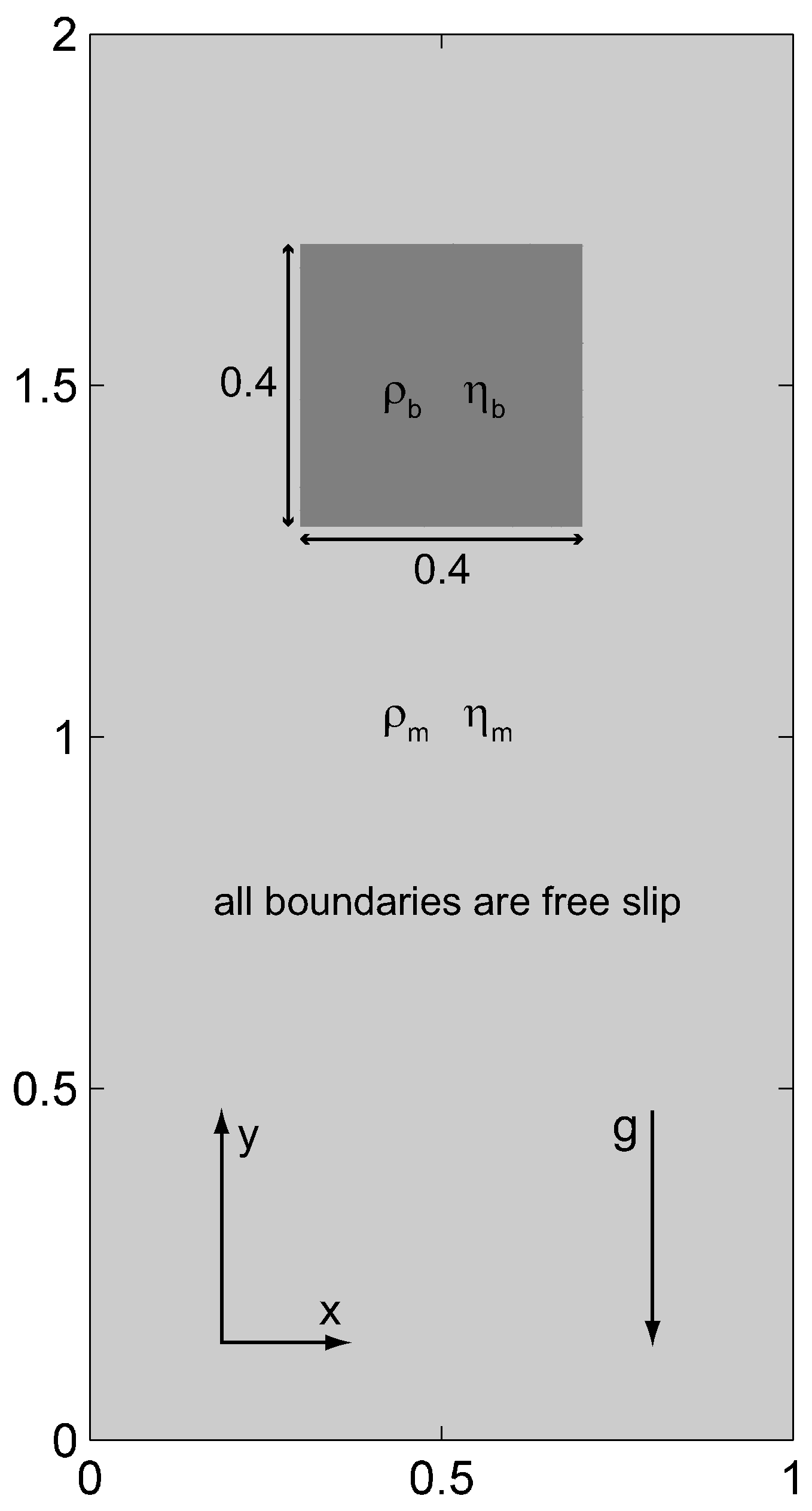
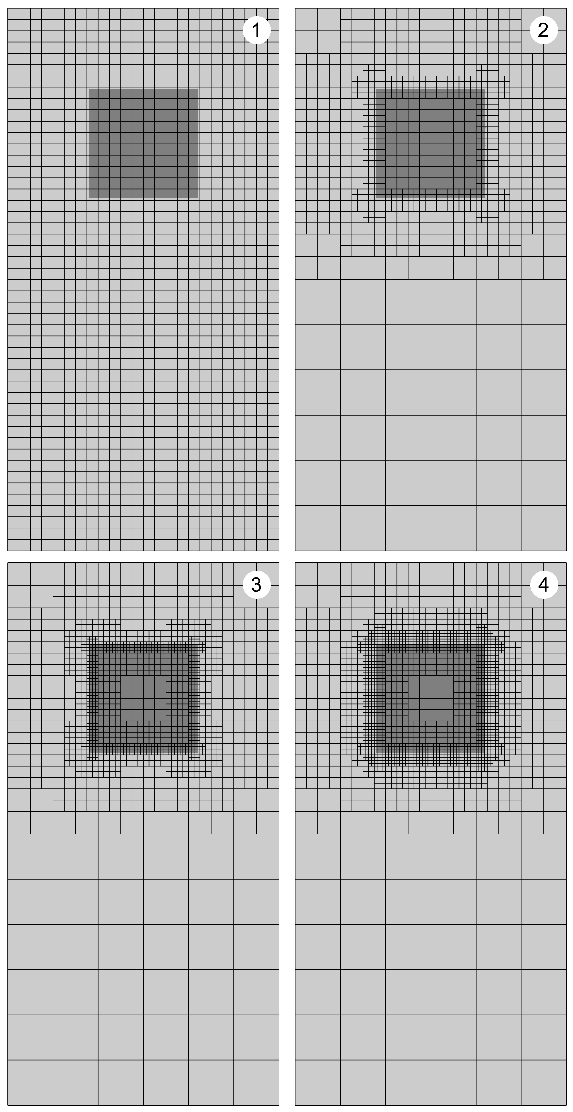
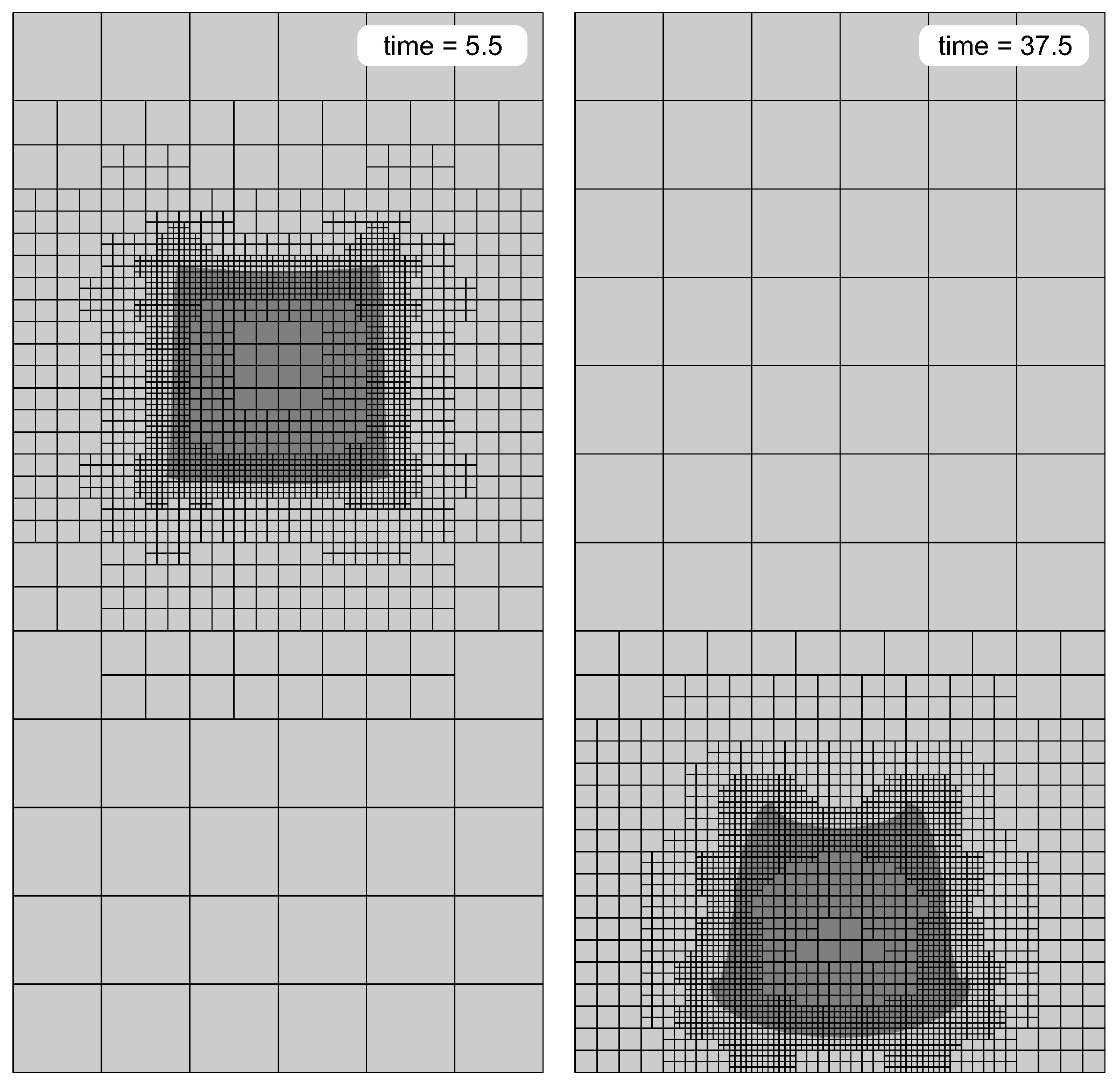
8.2. Sinking Block Benchmark

To evaluate the general applicability of the proposed adaptive numerical method, we performed the classical numerical benchmark of a sinking of a hard rectangular block into a medium with a lower viscosity [26]. Although corresponding analytical solution is not known, the numerical results can be evaluated in a qualitative sense.

8.2.1. Setup and Parameters

The model setup is shown on Figure 12, and employed physical and numerical parameters are provided in

Table 2. Model parameters for the sinking block benchmark.

Parameter	Value
Block viscosity ${\eta }_{\mathrm{b}}$	${10}^2–{10}^7$
Medium viscosity ${\eta }_{\mathrm{m}}$	$1.0$
Block density ${\rho }_{\mathrm{b}}$	$2.0$
Medium density ${\rho }_{\mathrm{m}}$	$1.0$
Gravitational acceleration g	$-10.0$
Time step $\Delta t$	$0.1$

. The numerical simulations were performed on ${\mathrm{Q}}_1{\mathrm{P}}_0$ and ${\mathrm{Q}}_1{\mathrm{Q}}_1$ adaptive grids of $6\times 12\to 96\times 192$ (5 levels) resolution, and with about $1.7\times {10}^5$ Lagrangian particles. The viscosity field was used as an adaptation criterion with an adaptation threshold $\epsilon ={10}^{-3}$.

Since the viscosity interface between the block and the medium exists a priori, the preliminary grid adaptation was performed before the actual numerical simulations were started (Figure 13).

8.2.2. Effect of Viscosity Contrast

The results of numerical simulations on ${\mathrm{Q}}_1{\mathrm{Q}}_1$ adaptive grid with ${10}^2$ and ${10}^7$ viscosity contrasts are shown on Figure 14 and Figure 15 respectively. As it is seen from the figures, the interface between the block and the medium is accurately captured by a multilevel grid as simulation proceeds and the block sinks down. As expected from the physical point of view, the block undergoes deformations in case of moderate viscosity contrast (${10}^2$), but these deformations vanish as viscosity contrast becomes high (${10}^7$). The fact that the shape of the block is preserved at high viscosity contrast also verifies that the implemented numerical scheme is stress conservative.

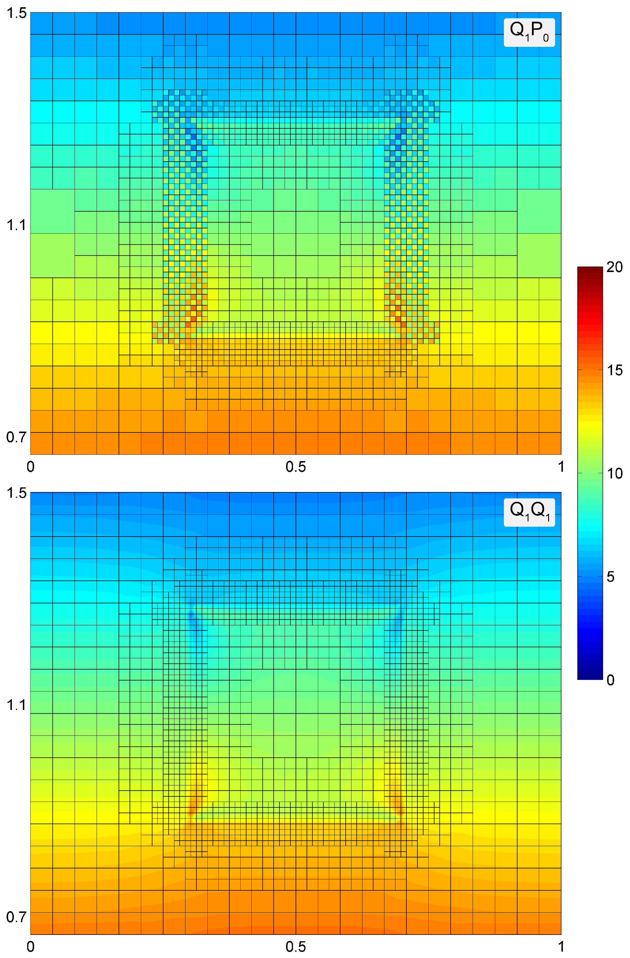
8.2.3. Checkerboard Pressure Problem with ${\mathrm{Q}}_1{\mathrm{P}}_0$ Element

The benchmark was performed using ${\mathrm{Q}}_1{\mathrm{P}}_0$ mixed approximation to evaluate its applicability and make a comparison with ${\mathrm{Q}}_1{\mathrm{Q}}_1$ element.

While the general model evolution is similar for ${\mathrm{Q}}_1{\mathrm{Q}}_1$ and ${\mathrm{Q}}_1{\mathrm{P}}_0$ elements, the pressure solution obtained with ${\mathrm{Q}}_1{\mathrm{P}}_0$ clearly shows strong checkerboard effect (Figure 16). This problem is well known and is caused by the fact that ${\mathrm{Q}}_1{\mathrm{P}}_0$ is inherently unstable [16,17]. However, in our experience, the checkerboard effect is even more evident when multilevel grid is employed. Thus, ${\mathrm{Q}}_1{\mathrm{P}}_0$ element has to be used with care, especially when non-linear pressure-dependent rheology is used (see Section 8.3).

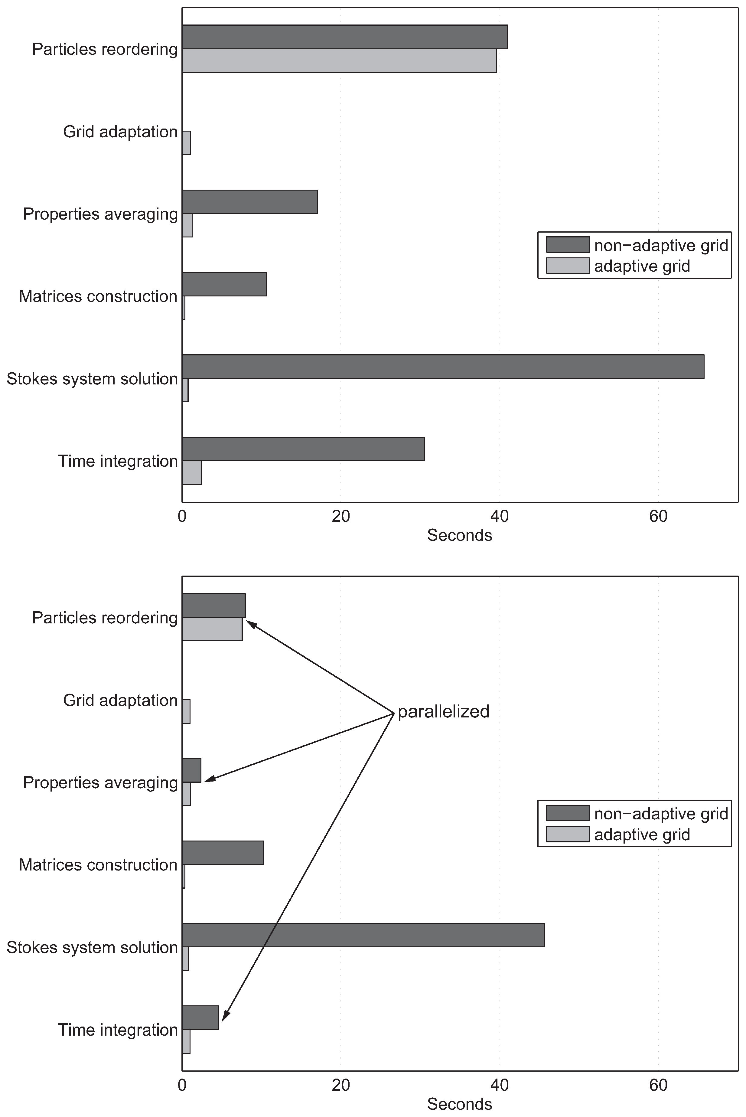
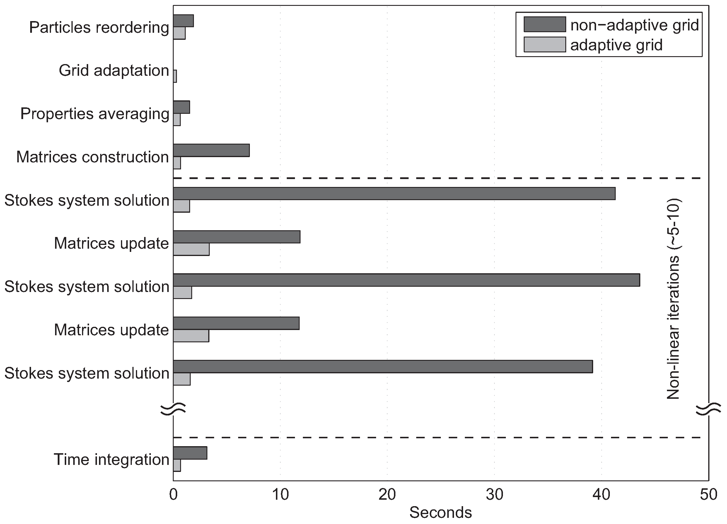
8.2.4. Performance Analysis

The comparisons of average performance between ${\mathrm{Q}}_1{\mathrm{Q}}_1$ adaptive and non-adaptive schemes were done at resolutions $6\times 12\to 384\times 768$ (7 levels) in adaptive and $384\times 768$ in non-adaptive case, and with about $2.7\times {10}^6$ Lagrangian particles in both cases. The results obtained in sequential (1 CPU) and parallel (8 CPUs) modes are shown on Figure 17.

As it is seen from the plots, there is a very significant performance gain when adaptation is employed, especially for the solution of the Stokes system. Due to the high cost of Voronoi tessellation, the reordering of Lagrangian particles is relatively expensive in both adaptive and non-adaptive cases. The potential solution to this problem is to implement the Voronoi tessellation functionality in an external library using a low-level language, such as C++.

The parallel speedup from 1 to 8 CPUs is significant but less than linear. This can be explained by the fact that MATLAB Parallel Computing Toolbox is a relatively new product, and an efficient parallelization using an interpreted dynamic language, such as MATLAB, poses significant challenges.

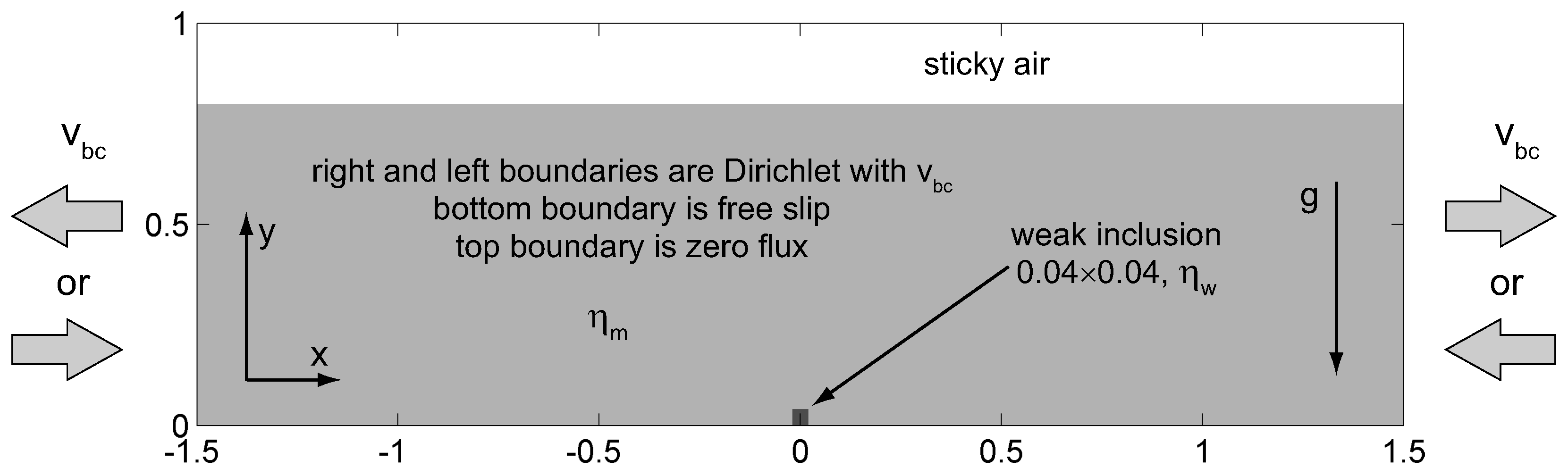
8.3. Brittle Extension/Compression Benchmark

This benchmark was performed to test the capabilities of the proposed adaptive approach to capture and resolve spontaneously forming shear zones in non-linear brittle faulting models.

8.3.1. Setup and Parameters

The extension/compression model setup is shown on Figure 18, and model parameters are given in

Table 3. Model parameters for brittle extension/compression benchmark.

Parameter		Value
	Weak inclusion viscosity ${\eta }_{\mathrm{w}}$	$1.0$
	Medium viscosity ${\eta }_{\mathrm{m}}$	$100.0$
	Weak inclusion and medium density $\rho$	$1.0$
	Air viscosity ${\eta }_{\mathrm{a}}$	$0.01$
	Air density ${\rho }_{\mathrm{a}}$	$0.0$
	Gravitational acceleration g	$-10.0$
	Friction angle $\varphi$	$0^{\circ }–{30}^{\circ }$
	Strain values ${\epsilon }_1/{\epsilon }_2$	$0.0/0.1$
Cohesion $c_1/c_2$	Extension	$4.0/1.0$
	Compression	$20.0/10.0$
Boundary velocity $v_{\mathrm{bc}}$	Extension	$0.05$
	Compression	$-0.5$
Time step $\Delta t$	Extension	$0.02$
	Compression	$0.004$
	Nonlinear tolerance ${ϵ}_{\mathrm{nl}}$	${10}^{-3}$

(physical parameters are from [14]). The numerical experiments were performed on ${\mathrm{Q}}_1{\mathrm{Q}}_1$-based $12\times 4\to 768\times 256$ (7 levels) adaptive and on $768\times 256$ non-adaptive grids, and with about $1.8\times {10}^6$ Lagrangian particles in both cases. Adaptive simulations were started on $384\times 128$ equidistant grid. The $v_x$- and $v_y$-velocity fields served as adaptation criteria with a threshold $\epsilon ={10}^{-3}$. Thus, the wavelet-based adaptation was performed independently for each of velocity fields, and the results were combined to form a common adapted mask. The multilevel grid, constructed from such a mask, efficiently captures the gradients of the strain rate field.

The strain softening/hardening behavior of brittle materials is modeled by adjusting the cohesion c at each time step as:

$$c=c_1+(c_2-c_1)min\left\{1,max\left\{0,\frac{{\epsilon }_{\mathrm{pl}}-{\epsilon }_1}{{\epsilon }_2-{\epsilon }_1}\right\}\right\}$$

(46)

Thus, the cohesion value c is changed linearly from initial $c_1$ to final $c_2$ as accumulated plastic strain ${\epsilon }_{pl}$ changes from ${\epsilon }_1$ to ${\epsilon }_2$. The softening behavior is imposed when $c_2<c_1$, and the hardening — when $c_2>c_1$. The accumulated plastic strain ${\epsilon }_{\mathrm{pl}}$ is defined on Lagrangian particles, and is integrated by the forward Euler scheme as other particles properties:

$${\epsilon }_{\mathrm{pl}}(t+\Delta t)={\epsilon }_{\mathrm{pl}}\left(t\right)+{\dot{\epsilon }}_{\mathrm{pl}}\left(t\right)\Delta t$$

(47)

Here ${\dot{\epsilon }}_{\mathrm{pl}}$ is the plastic strain rate computed as:

$${\dot{\epsilon }}_{\mathrm{pl}}={\dot{\epsilon }}_{II}\left(1-\frac{{\eta }_{\mathrm{eff}}}{{\eta }_{\mathrm{creep}}}\right)$$

(48)

where ${\dot{\epsilon }}_{II}$ is the second invariant of the strain rate tensor, and ${\eta }_{\mathrm{creep}}$ and ${\eta }_{\mathrm{eff}}$ and creep and viscoplastic effective viscosities respectively.

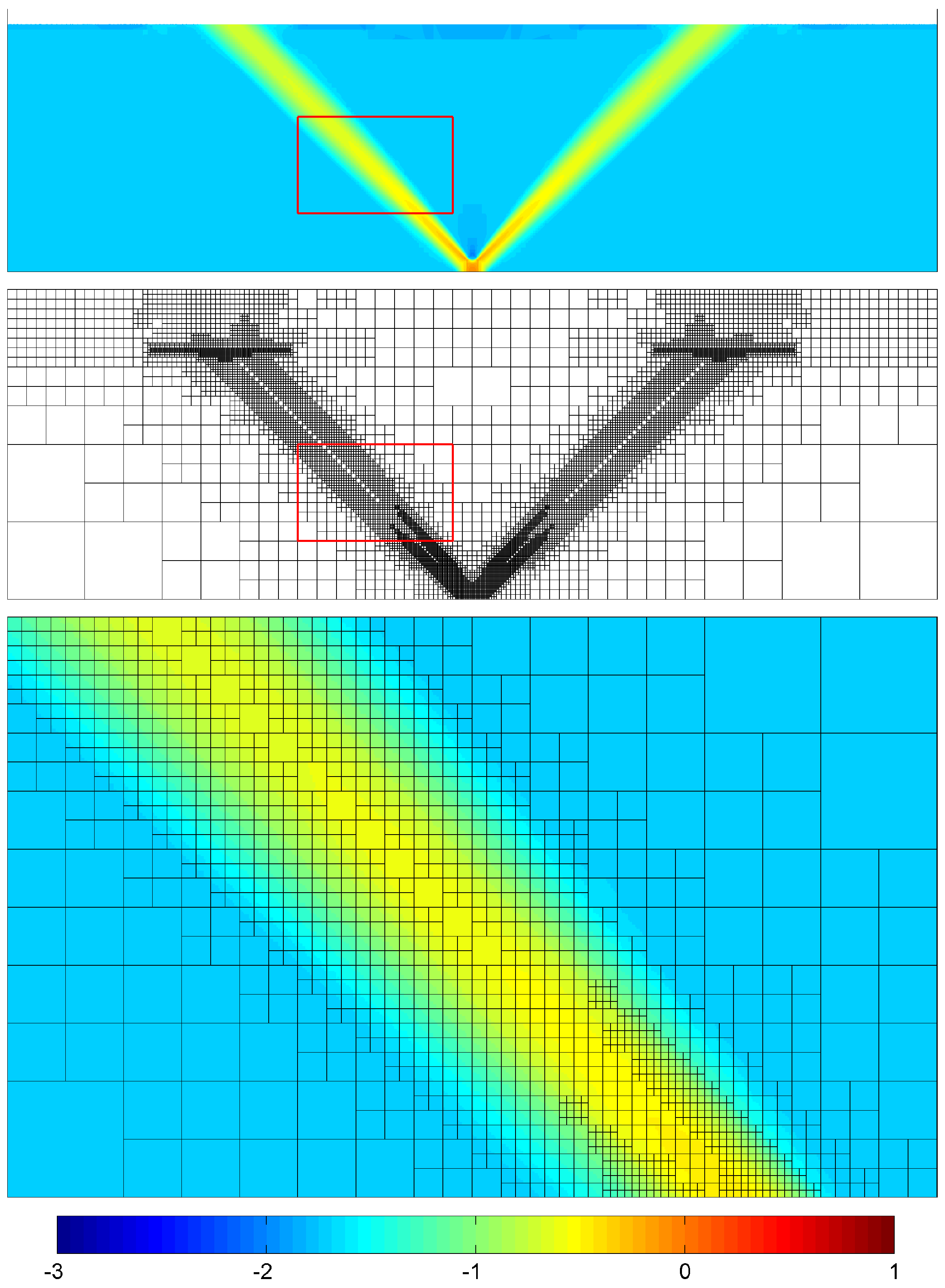
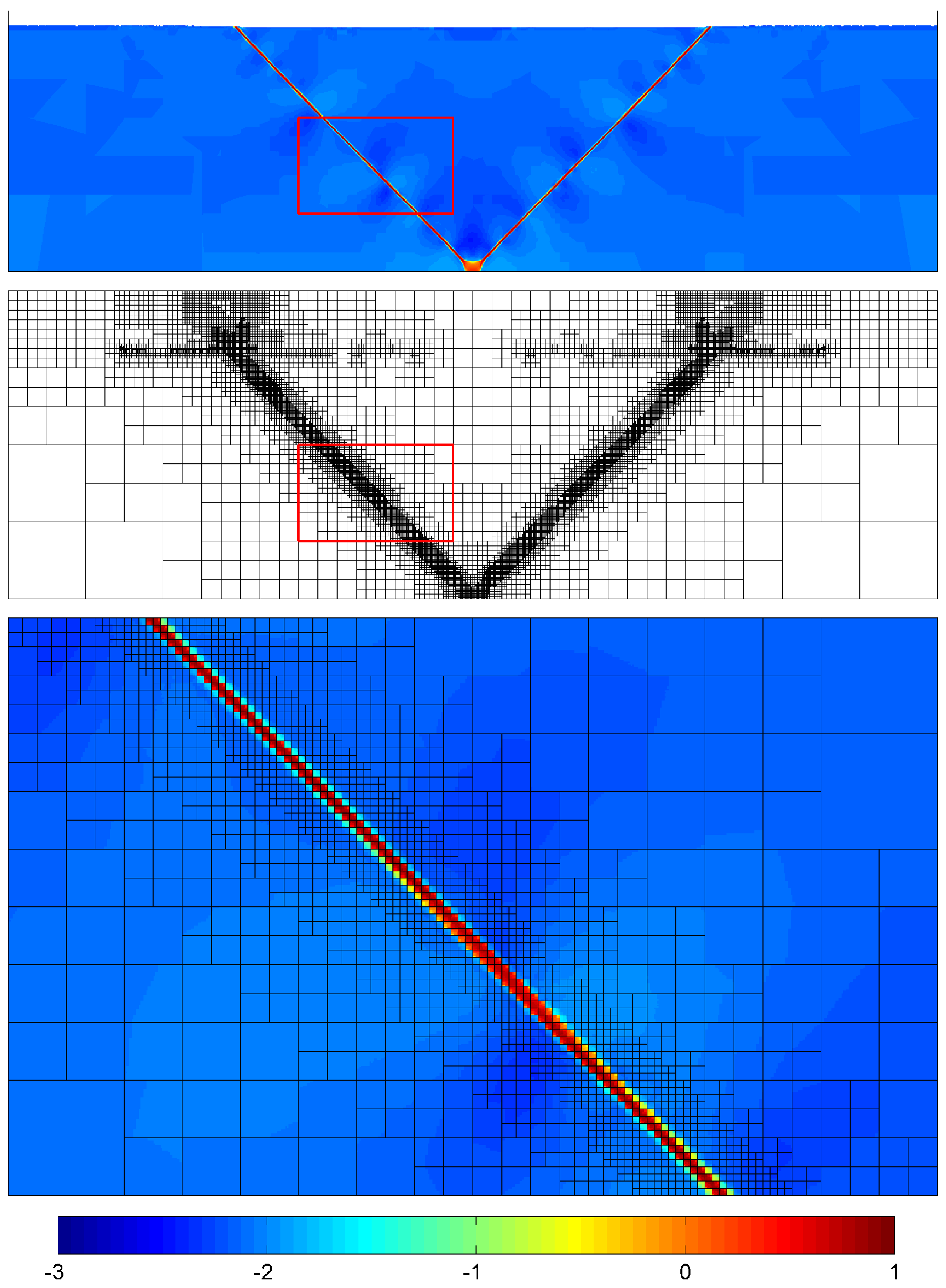
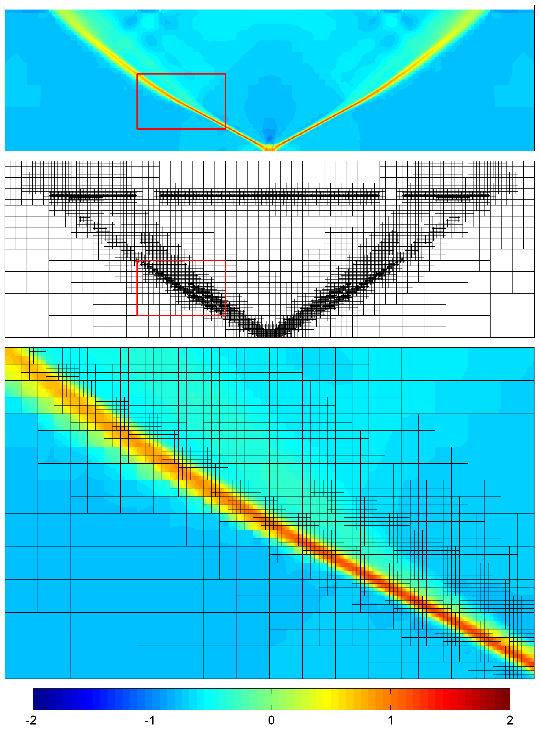
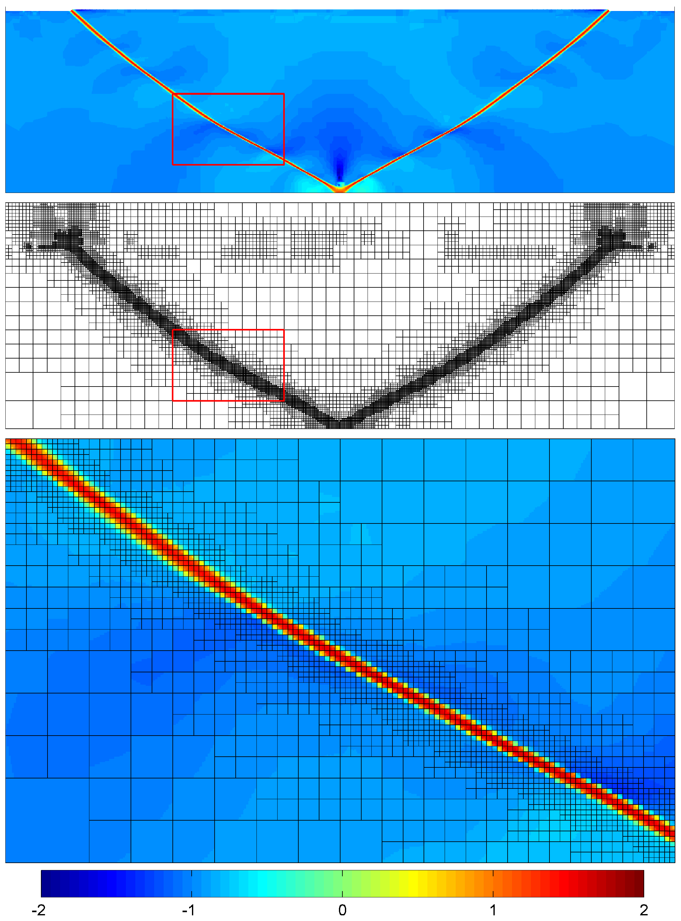
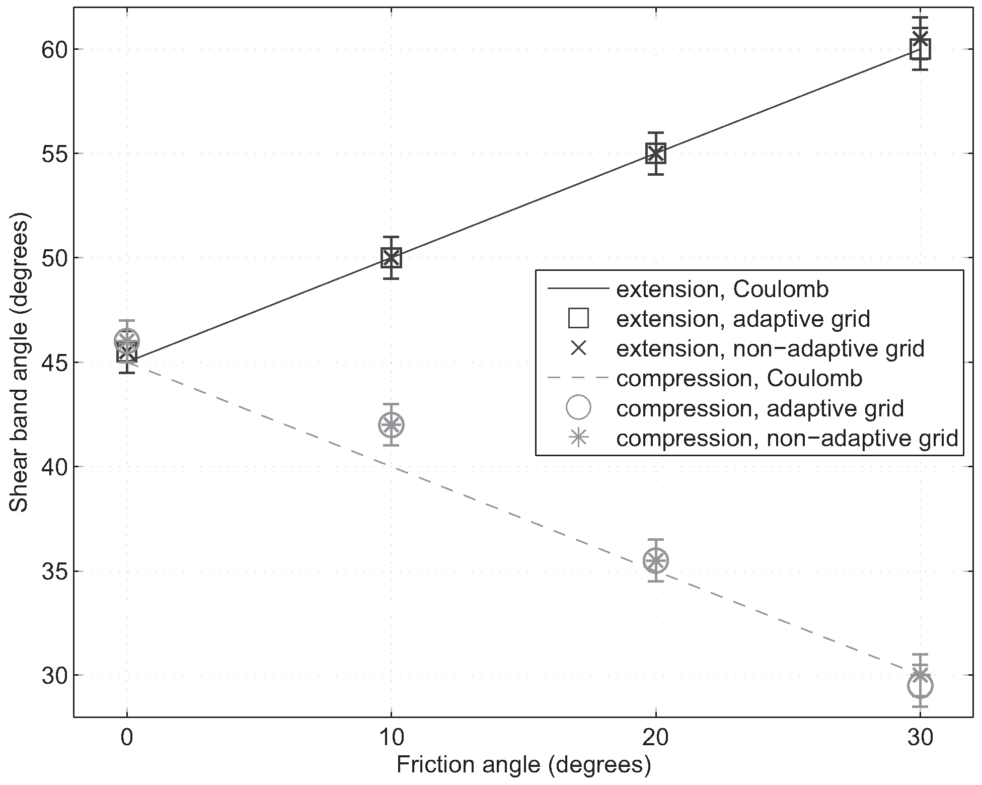
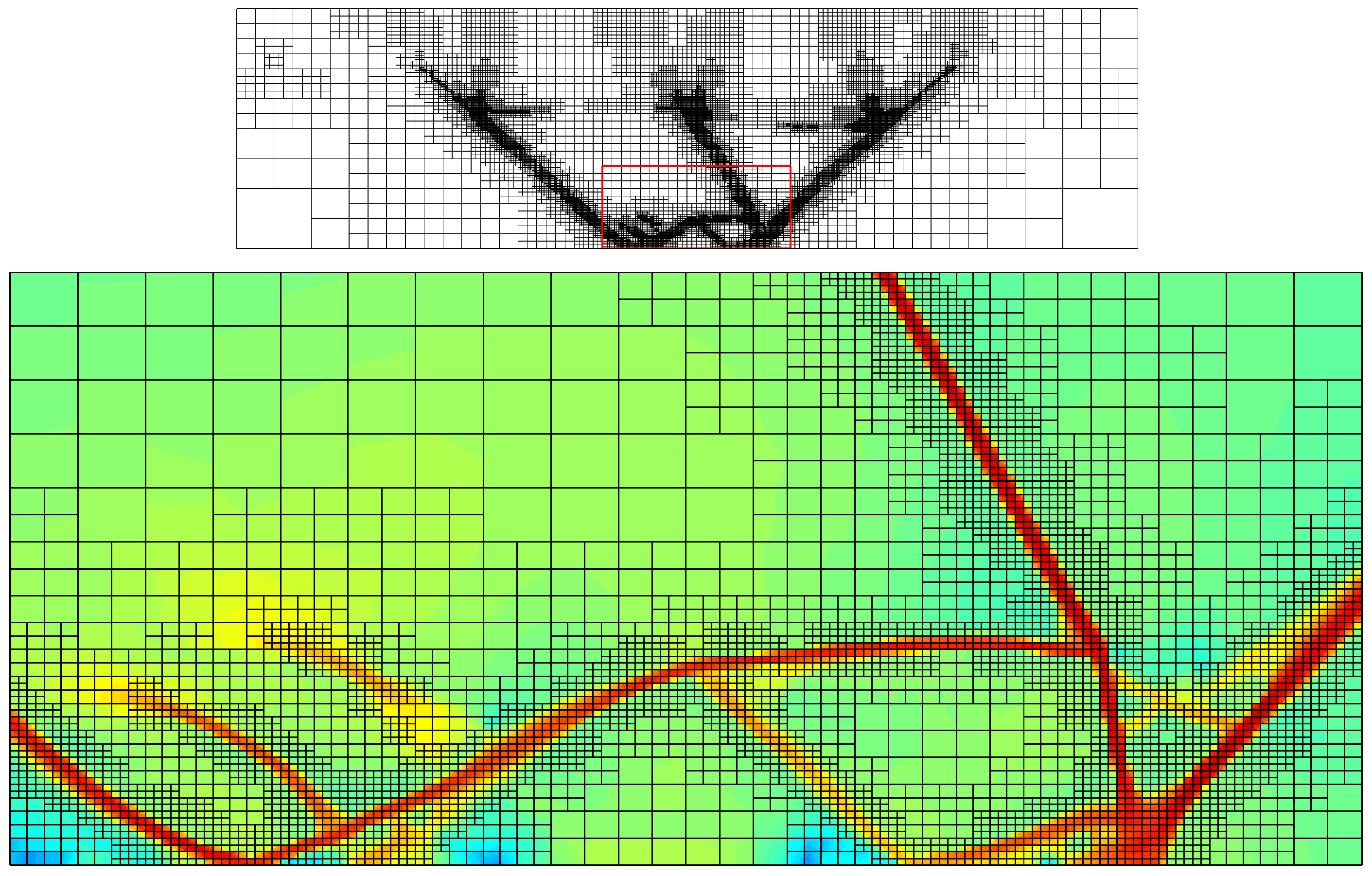
8.3.2. Shear Bands Formation

The brittle extension and compression numerical experiments were performed with friction angles $\varphi =0^{\circ }$, ${10}^{\circ }$, ${20}^{\circ }$ and ${30}^{\circ }$ on both adaptive and non-adaptive grids. As an example, the results of an extension numerical simulation with $\varphi =0^{\circ }$ are shown on Figure 19 and Figure 20, and the results of a compression simulation with $\varphi ={30}^{\circ }$ are shown on Figure 21 and Figure 22. As it is seen from the figures, the multilevel grid is progressively adapted to capture and better resolve appearing brittle faults as simulation proceeds.

The orientations of the formed shear bands with respect to horizontal were measured for both adaptive and non-adaptive models and compared against each other and against Coulomb orientations (Figure 23). The results obtained on adaptive and non-adaptive grids are very close, and show good agreement with Coulomb angles which are expected [14,42].

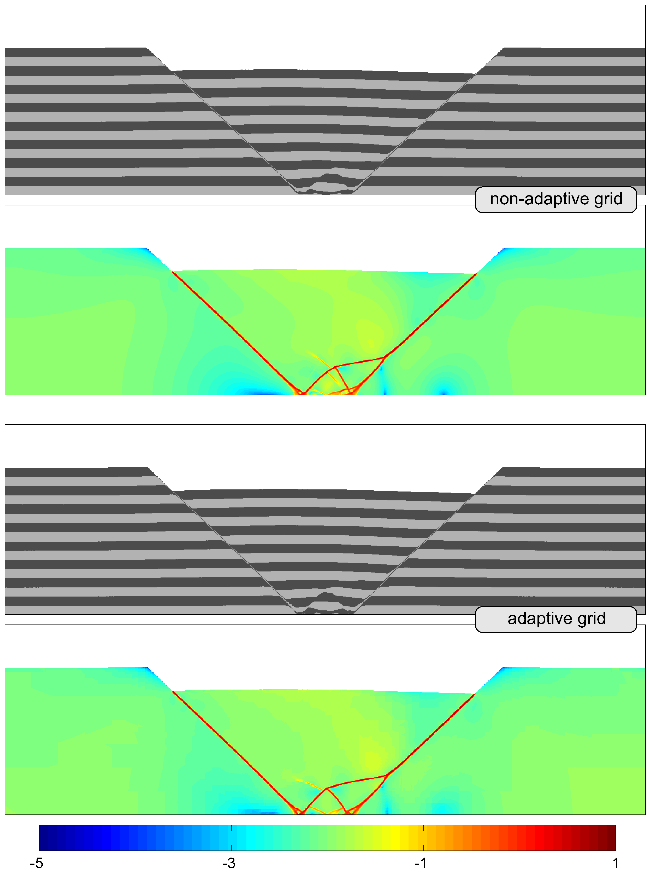
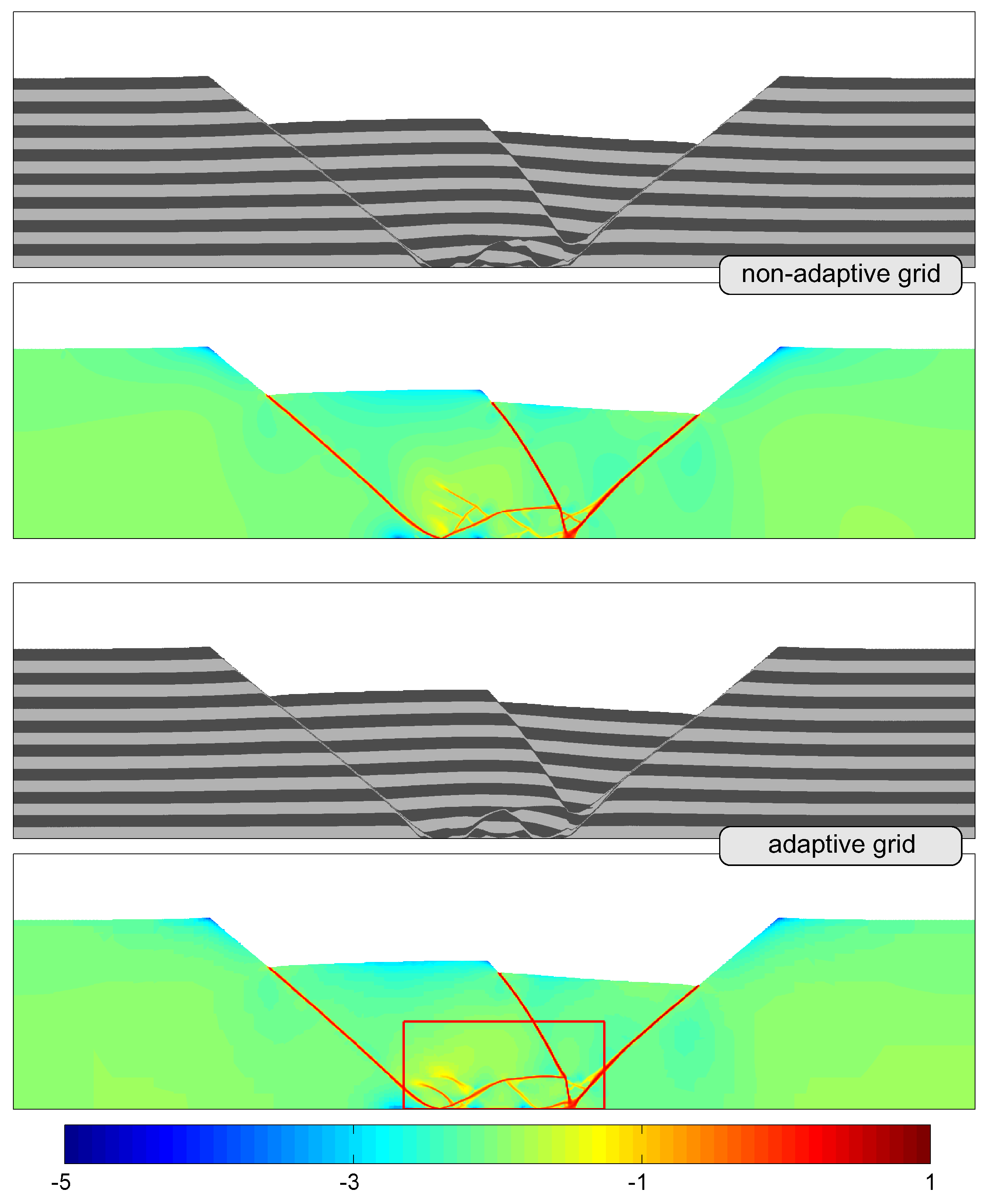
8.3.3. Long-Term Brittle Extension

It is interesting to compare long-term brittle model evolution simulated on adaptive and non-adaptive grids. The material and strain rate fields from extension simulations with $\varphi =0^{\circ }$ after relatively high strains are shown on Figure 24, Figure 25 and Figure 26. As it is seen from the figures, the results obtained on adaptive and non-adaptive grids are almost identical. Thus, for considered models, the adaptive scheme can be used instead of non-adaptive with confidence.

8.3.4. Performance Analysis

The comparison of average performance between adaptive and non-adaptive schemes is shown on Figure 27. As in the sinking block benchmark (Section 8.2), the performance gain for matrices construction and Stokes system solution is very significant when adaptive grid is employed. However, the considered problem is non-linear and the Stokes system has to be constructed and solved normally more than once at each time step. Thus, the overall performance advantage of the adaptive approach is even more dramatic in this case.

8.4. Incompressibility Issue with $Q_1{Q}_1$ Element

As was demonstrated by previous numerical experiments (Section 8.2 and Section 8.3), the results obtained with stabilized ${\mathrm{Q}}_1{\mathrm{Q}}_1$ element are adequate in many cases. However, in many gravity-driven geodynamic models, the ${\mathrm{Q}}_1{\mathrm{Q}}_1$ element behaves unreliably due to the issue of artificial incompressibility caused by the addition of the stabilization matrix $\mathbf{V}$ to the Stokes system. This problem is discussed in the original works [18,19] and was also confirmed in personal communications with P. Bochev.

To evaluate the issue, we performed the series of numerical simulations on ${\mathrm{Q}}_1{\mathrm{Q}}_1$- and ${\mathrm{Q}}_2{\mathrm{P}}_{-1}$-based regular grids of a model containing square $1.0\times 1.0$ domain with uniform $\rho =1.0$ and $\eta =1.0$ and applied gravity $g=-10.0$. Since the media is assumed to be incompressible, one would expect $v_y$-velocity to be zero everywhere. However, the differences between normalized $L^2$-norms of $v_y$ obtained with ${\mathrm{Q}}_1{\mathrm{Q}}_1$ and ${\mathrm{Q}}_2{\mathrm{P}}_{-1}$ elements are almost 10 orders of magnitude (

Table 4. Velocity norms ${\parallel v_y\parallel }_2$ normalized by the number of elements.

Element Type	Resolution
	$\mathbf{100}\times \mathbf{100}$	$\mathbf{200}\times \mathbf{200}$	$\mathbf{400}\times \mathbf{400}$	$\mathbf{800}\times \mathbf{800}$
${\mathrm{Q}}_1{\mathrm{Q}}_1$	$8.35\times {10}^{-7}$	$1.04\times {10}^{-7}$	$1.30\times {10}^{-8}$	$1.63\times {10}^{-9}$
${\mathrm{Q}}_2{\mathrm{P}}_{-1}$	$2.26\times {10}^{-17}$	$2.31\times {10}^{-17}$	$2.39\times {10}^{-17}$	$2.89\times {10}^{-17}$

).

Thus, while the ${\mathrm{Q}}_1{\mathrm{Q}}_1$ element is stable and can be efficiently used in numerical experiments like brittle faulting (Section 8.3), it has to be avoided in models which are gravity-driven by a small density differences—such as Rayleigh-Taylor instability or subduction simulations.

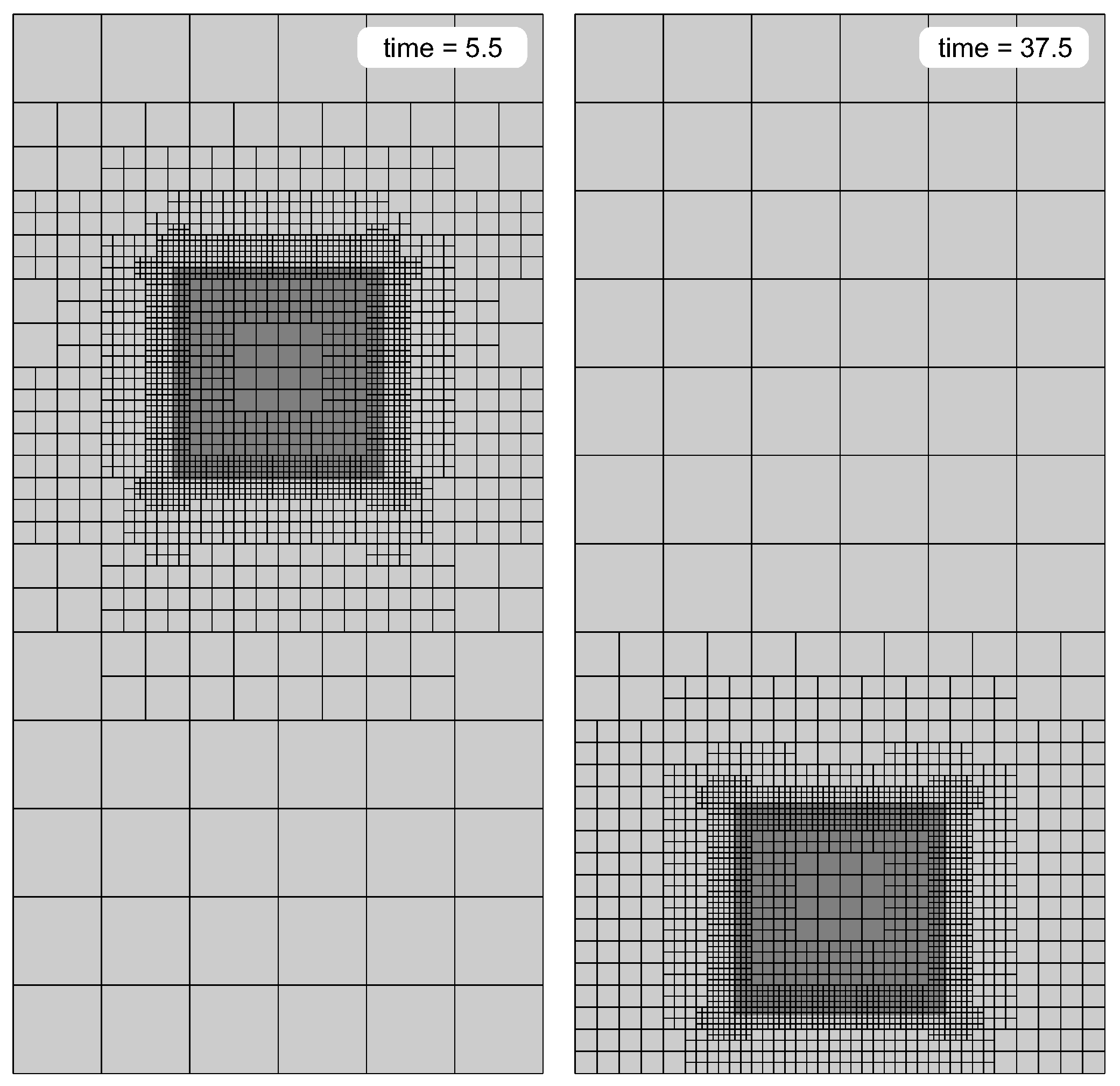
8.5. Rayleigh-Taylor Instability Benchmark

This is the classical two-layer Rayleigh-Taylor instability benchmark. The corresponding analytical solution is available, and thus the accuracy of the employed computational scheme can be evaluated.

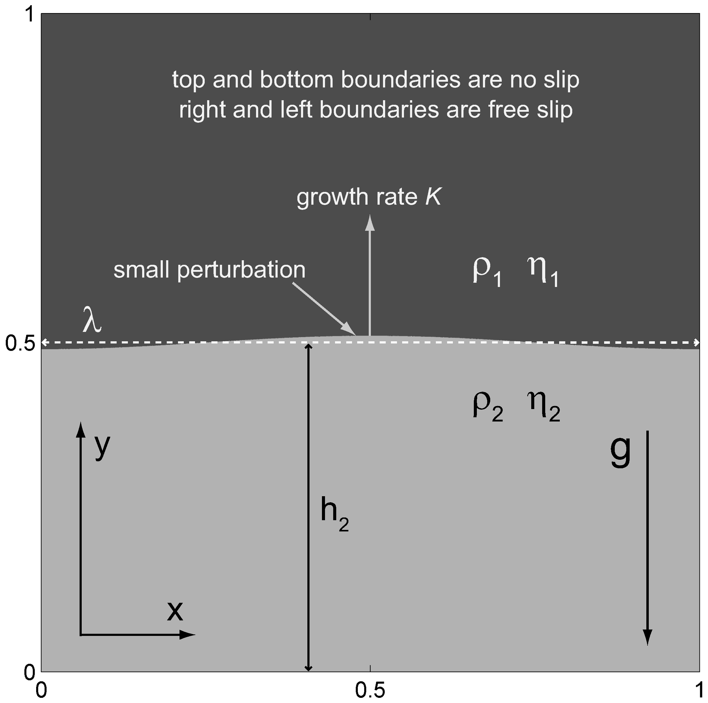
8.5.1. Setup and Parameters

The Rayleigh-Taylor model setup is shown on Figure 28, and model parameters are provided in

Table 5. Model parameters for the Rayleigh-Taylor benchmark.

Parameter	Value
Top layer viscosity ${\eta }_1$	$1–2000$
Bottom layer viscosity ${\eta }_2$	$1–1000$
Top layer density ${\rho }_1$	$1.1$
Bottom layer density ${\rho }_2$	$1.0$
Gravitational acceleration g	$-10.0$
Courant number	$0.8$

. The ${\mathrm{Q}}_1{\mathrm{Q}}_1$ element can not be used for this benchmark due to incompressibility issue (see above), and thus biquadratic mixed approximation ${\mathrm{Q}}_2{\mathrm{P}}_{-1}$ was used. The numerical simulations were performed on $25\times 25\to 400\times 400$ (5 levels) adaptive and on $400\times 400$ non-adaptive grids, and with $1.6\times {10}^7$ Lagrangian particles in both cases. The material density field was used as an adaptation criterion with a threshold $\epsilon ={10}^{-5}$. Since the density interface between the layers exists a priori, the preliminary grid adaptation was performed—as in the sinking block benchmark.

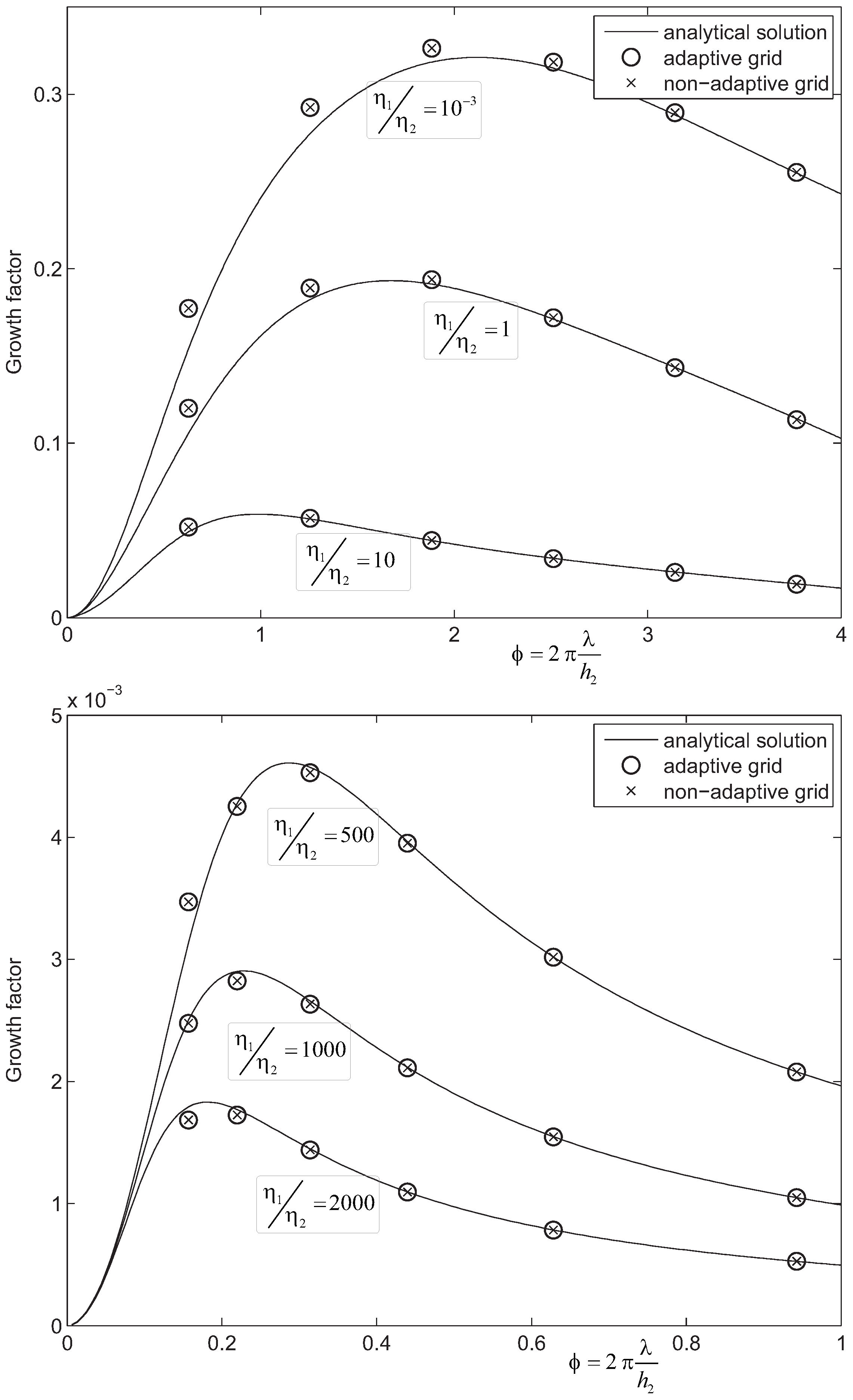
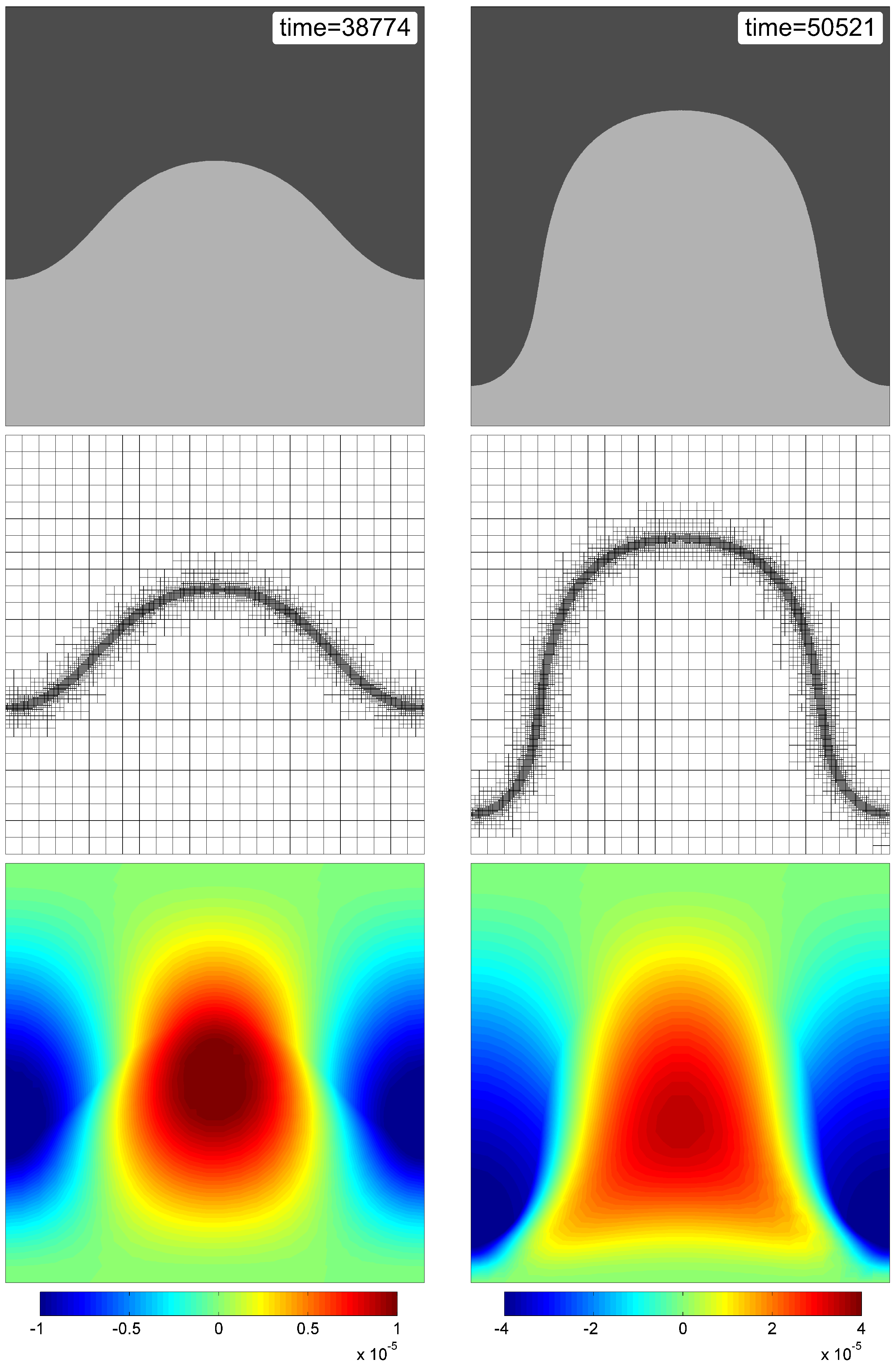
8.5.2. Growth of Diapirs

The series of Rayleigh-Taylor numerical simulations were performed varying viscosity contrast $\frac{{\eta }_1}{{\eta }_2}$ and thickness of bottom layer $h_2$ on both adaptive and non-adaptive grids. The growth factors were calculated after the first time step for both adaptive and non-adaptive models and compared against each other and against analytical solution [43,44], the results are provided on Figure 29. As it is seen from the plots, growth factors obtained on adaptive and non-adaptive grids are practically equal, and good agreement with analytical solution is observed.

To illustrate the following diapiric growth, some results for subsequent simulation time steps are shown on Figure 30, Figure 31 and Figure 32. As it is seen from the figures, the interface between the layers remains accurately captured and resolved by an adaptive grid as simulation proceeds.

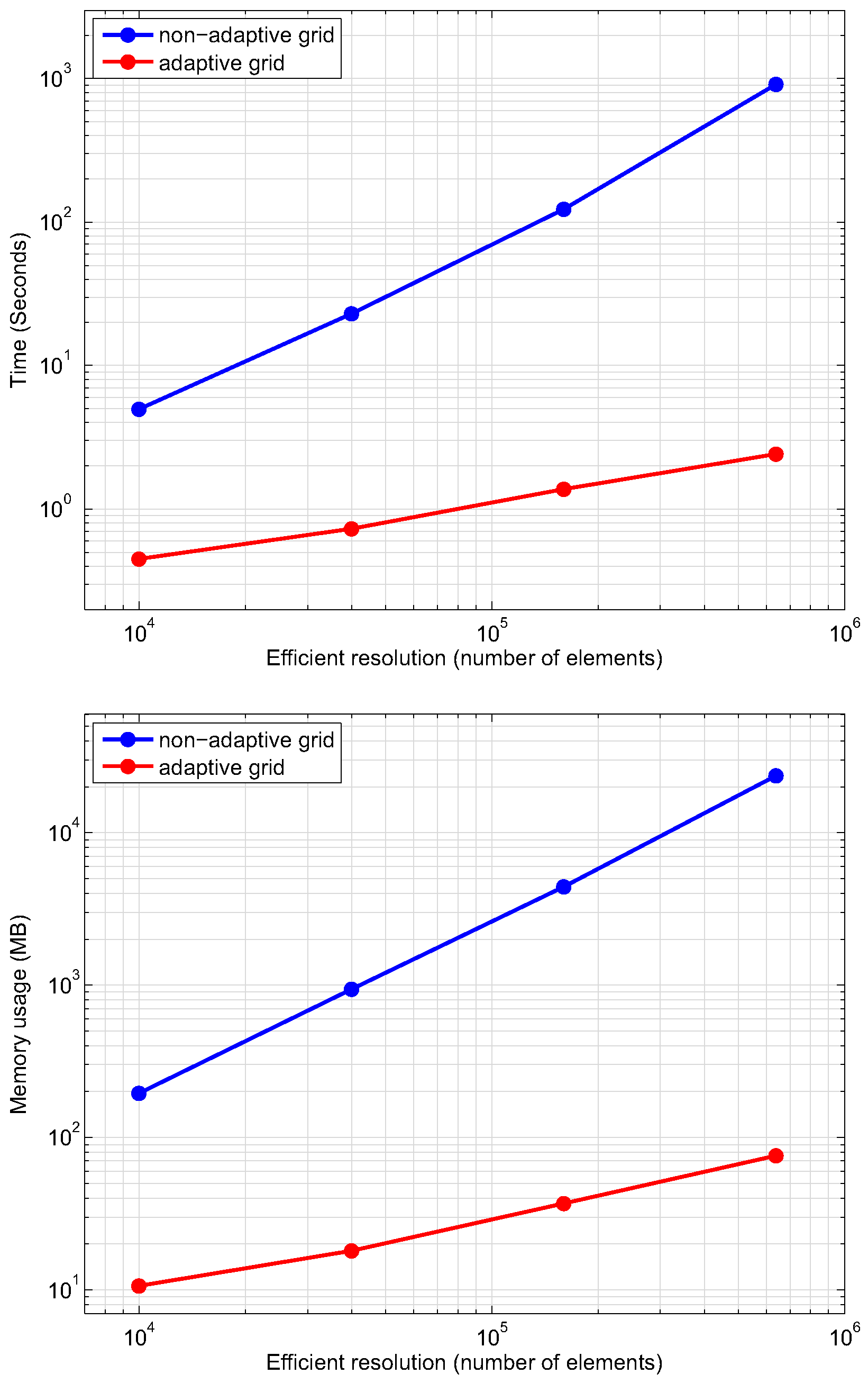
8.5.3. Performance Analysis

The plots provided on Figure 33 show the measured time and memory requirements for a single Cholesky factorization for numerical simulations on adaptive and non-adaptive grids of $100\times 100$, $200\times 200$, $400\times 400$ and $800\times 800$ efficient numerical resolutions. The power of adaptive approach is evident—both time and memory requirements can differ by as high as 3 orders of magnitude (the $800\times 800$ case).

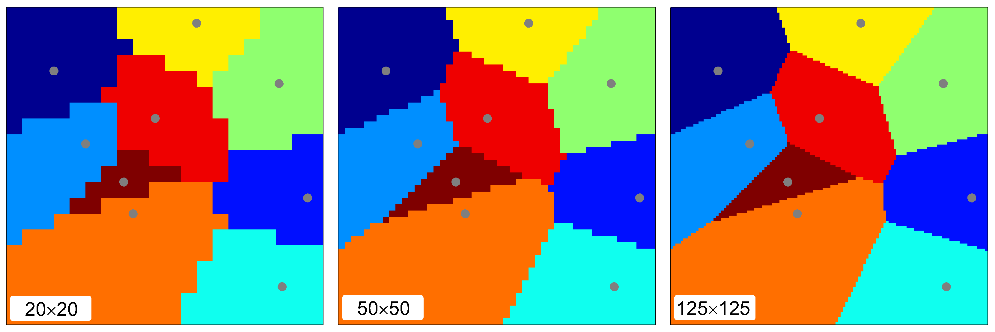
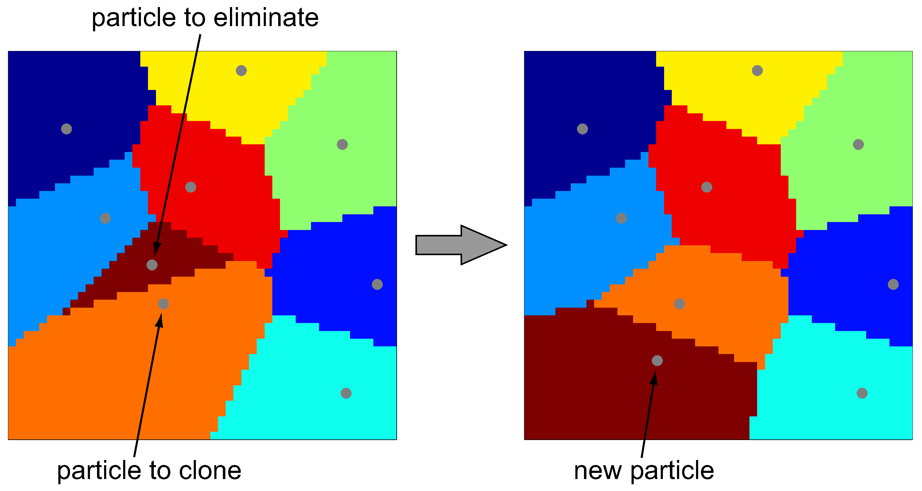
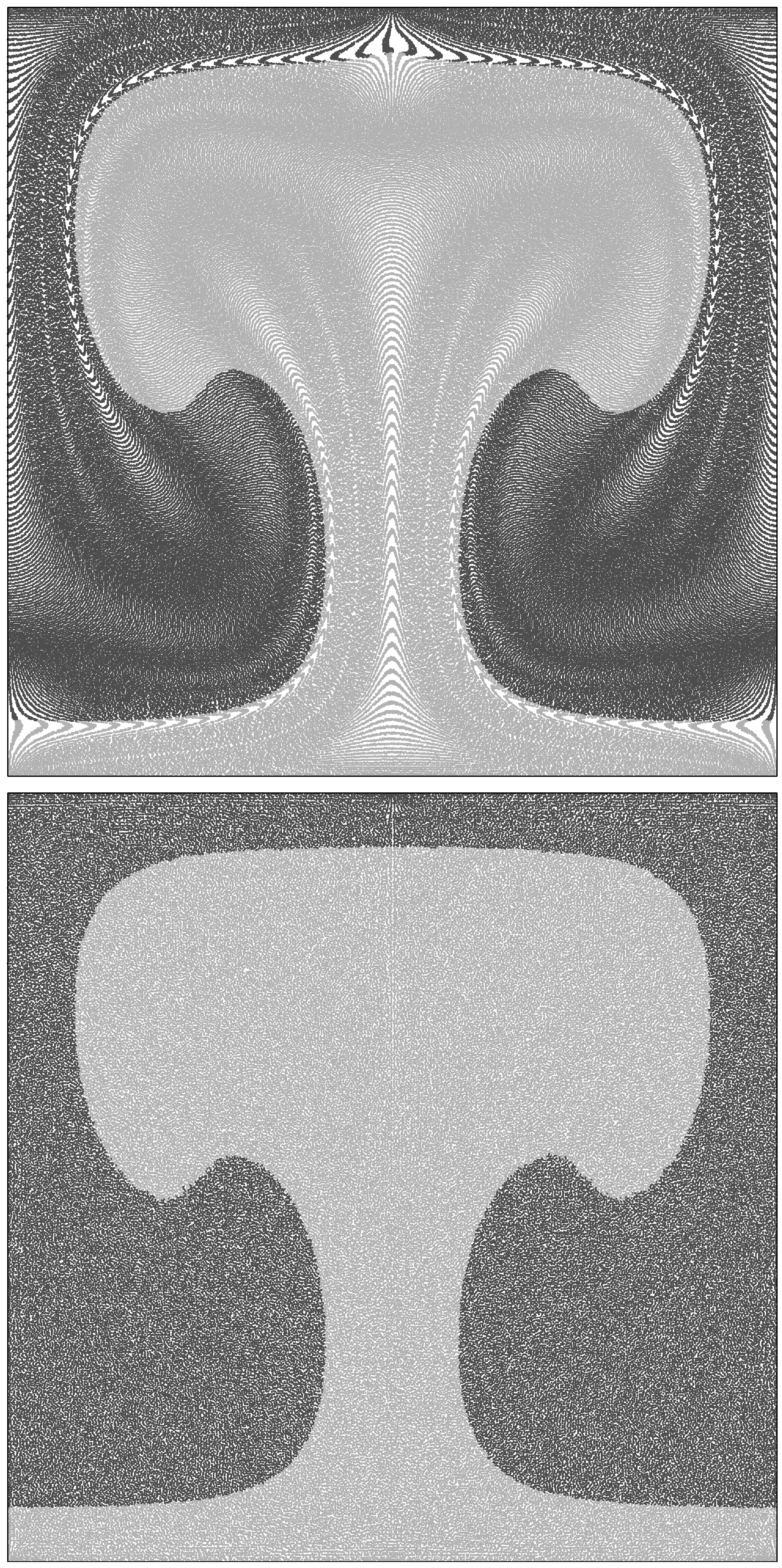
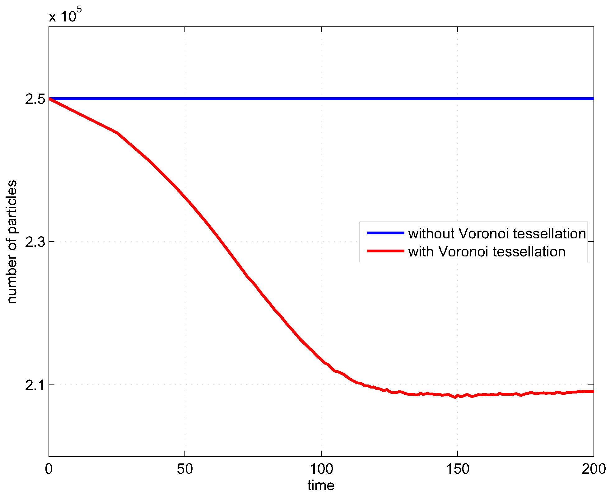
8.5.4. Effect of Voronoi Tessellation

Due to the relatively large deformations, the Rayleigh-Taylor instability benchmark serves as a good test to check the efficiency of the Voronoi tessellation algorithm to maintain uniform distribution of Lagrangian particles. The numerical simulations of diapiric growth with and without Voronoi algorithm were performed on ${\mathrm{Q}}_2{\mathrm{P}}_{-1}$-based $25\times 25\to 100\times 100$ (3 levels) adaptive grid, and with $2.5\times {10}^5$ Lagrangian particles. For the experiment with enabled Voronoi tessellation, the minimum and maximum cell areas were $A{V}_{min}=\frac{1}{50}$ and $A{V}_{max}=\frac{1}{12}$. The effect of the Voronoi algorithm on a Lagrangian particle distribution is illustrated on Figure 34, and dependency plot of the number of particles on time is provided on Figure 35. As it is seen from the Figure 34, the Voronoi tessellation algorithm works very efficiently in keeping uniform particle density across the domain.

9. Conclusions

In this work, a new adaptive multiresolution finite element method for the Stokes flow problems is presented (the implementation is available for download from http://sites.google.com/site/sdvigus/ (last accessed on 28 June 2022)). The automatic grid adaptation is supported for bilinear and biquadratic mixed discretizations and is implemented using an original algorithm based on wavelet analysis [4,6]. The proposed method was applied to linear (lateral viscosity variation, sinking block and Rayleigh-Taylor instability benchmarks) and to non-linear (brittle extension/compression benchmark) problems. The obtained numerical results are shown to be in an excellent agreement with those obtained on non-adaptive grids and with analytical solutions. At the same time, computational requirements of the method are up to few orders of magnitude lower compared to the non-adaptive grid approach, in terms of both time and memory usage.

References

1. Albers, M. A Local Mesh Refinement Multigrid Method for 3-D Convection Problems with Strongly Variable Viscosity. J. Comput. Phys. 2000, 160, 126–150. [Google Scholar] [CrossRef]
2. Stadler, G.; Gurnis, M.; Burstedde, C.; Wilcox, L.C.; Alisic, L.; Ghattas, O. The Dynamics of Plate Tectonics and Mantle Flow: From Local to Global Scales. Science 2010, 329, 1033–1038. [Google Scholar] [CrossRef] [PubMed]
3. Gerya, T.V.; May, D.A.; Duretz, T. An adaptive staggered grid finite difference method for modeling geodynamic Stokes flows with strongly variable viscosity. Geochem. Geophys. Geosyst. 2013, 14, 1200–1225. [Google Scholar] [CrossRef]
4. Vasilyev, O.V.; Bowman, C. Second-Generation Wavelet Collocation Method for the Solution of Partial Differential Equations. J. Comput. Phys. 2000, 165, 660–693. [Google Scholar] [CrossRef] [Green Version]
5. Vasilyev, O.V. Solving Multi-Dimensional Evolution Problems with Localized Structures Using Second Generation Wavelets. Int. J. Comp. Fluid Dyn. 2003, 17, 151–168. [Google Scholar] [CrossRef]
6. Vasilyev, O.V.; Gerya, T.V.; Yuen, D.A. The application of multidimensional wavelets to unveiling multi-phase diagrams and in situ physical properties of rocks. Earth Planet. Sci. Lett. 2004, 223, 49–64. [Google Scholar] [CrossRef]
7. Schneider, K.; Vasilyev, O.V. Wavelet Methods in Computational Fluid Dynamics. Ann. Rev. Fluid Mech. 2010, 42, 473–503. [Google Scholar] [CrossRef] [Green Version]
8. Nejadmalayeri, A.; Vezolainen, A.; Brown-Dymkoski, E.; Vasilyev, O.V. Parallel Adaptive Wavelet Collocation Method for PDEs. J. Comp. Phys. 2015, 298, 237–253. [Google Scholar] [CrossRef] [Green Version]
9. Ranalli, G. Rheology of the Earth; Chapman and Hall: London, UK, 1995. [Google Scholar]
10. Fullsack, P. An arbitrary Lagrangian-Eulerian formulation for creeping flows and its application in tectonic models. Geophys. J. Int. 1995, 120, 1–23. [Google Scholar] [CrossRef] [Green Version]
11. Moresi, L.; Solomatov, V. Mantle convection with a brittle lithosphere: Thoughts on the global tectonic styles of the Earth and Venus. Geophys. J. Int. 1998, 133, 669–682. [Google Scholar] [CrossRef]
12. Tackley, P.J. Self-consistent generation of tectonic plates in time-dependent, three-dimensional mantle convection simulations, 1, Pseudoplastic yielding. Geochem. Geophys. Geosyst. 2000, 1. [Google Scholar]
13. Chakrabarty, J. Theory of Plasticity; Butterworth-Heinemann: Oxford, UK, 2006. [Google Scholar]
14. Lemiale, V.; Mühlhaus, H.B.; Moresi, L.; Stafford, J. Shear banding analysis of plastic models formulated for incompressible viscous flows. Phys. Earth Planet. Inter. 2008, 171, 177–186. [Google Scholar] [CrossRef]
15. Zienkiewicz, O.C.; Morgan, K. Finite Elements and Approximation; Wiley: New York, NY, USA, 1983. [Google Scholar]
16. Fortin, M.; Brezzi, F. Mixed and Hybrid Finite Element Methods; Springer: New York, NY, USA, 1991. [Google Scholar]
17. Elman, H.C.; Silvester, D.J.; Wathen, A.J. Finite Elements and Fast Iterative Solvers; Oxford University Press: Oxford, UK, 2005. [Google Scholar]
18. Dohrmann, C.R.; Bochev, P.B. A stabilized finite element method for the Stokes problem based on polynomial pressure projections. Int. J. Num. Meth. Fluids 2004, 46, 183–201. [Google Scholar] [CrossRef] [Green Version]
19. Bochev, P.B.; Dohrmann, C.R.; Gunzburger, M.D. Stabilization of low-order mixed finite elements for the Stokes equations. SIAM J. Num. Anal. 2006, 44, 82–101. [Google Scholar] [CrossRef]
20. Zienkiewicz, O.C.; Taylor, R.L.; Zhu, J.Z. The Finite Element Method: Its Basis and Fundamentals; Butterworth-Heinemann: Oxford, UK, 2005. [Google Scholar]
21. Zienkiewicz, O.C.; Vilotte, J.P.; Toyoshima, S.; Nakazawa, S. Iterative method for constrained and mixed approximation. An inexpensive improvement of FEM performance. Comp. Meth. Appl. Mech. Eng. 1985, 51, 3–29. [Google Scholar] [CrossRef]
22. Dabrowski, M.; Krotkiewski, M.; Schmid, D.W. MILAMIN: MATLAB-based finite element method solver for large problems. Geochem. Geophys. Geosyst. 2008, 9, Q04030. [Google Scholar] [CrossRef]
23. Schmid, D.W.; Dabrowski, M.; Krotkiewski, M. Evolution of large amplitude 3D fold patterns: A FEM study. Phys. Earth Planet. Inter. 2008, 171, 400–408. [Google Scholar] [CrossRef]
24. May, D.A.; Moresi, L. Preconditioned iterative methods for Stokes flow problems arising in computational geodynamics. Phys. Earth Planet. Inter. 2008, 171, 33–47. [Google Scholar] [CrossRef]
25. Cuvelier, C.; Segal, A.; van Steenhoven, A.A. Finite Element Methods and Navier-Stokes Equations; Reidel: Dordrecht, The Netherlands, 1986. [Google Scholar]
26. Gerya, T.V.; Yuen, D.A. Characteristics-based marker-in-cell method with conservative finite-differences schemes for modeling geological flows with strongly variable transport properties. Phys. Earth Planet. Inter. 2003, 140, 293–318. [Google Scholar] [CrossRef]
27. Gerya, T.V.; Yuen, D.A. Robust characteristics method for modelling multiphase visco-elasto-plastic thermo-mechanical problems. Phys. Earth Planet. Inter. 2007, 163, 83–105. [Google Scholar] [CrossRef]
28. O’Neill, C.; Moresi, L.; Müller, D.; Albert, R.; Dufour, F. Ellipsis 3D: A particle-in-cell finite-element hybrid code for modelling mantle convection and lithospheric deformation. Comp. and Geosci. 2006, 32, 1769–1779. [Google Scholar] [CrossRef] [Green Version]
29. Gerya, T.V. Introduction to Numerical Geodynamic Modelling; Cambridge University Press: Cambridge, UK, 2010. [Google Scholar]
30. OzBench, M.; Regenauer-Lieb, K.; Stegman, D.R.; Morra, G.; Farrington, R.; Hale, A.; May, D.A.; Freeman, J.; Bourgouin, L.; Mühlhaus, H.; et al. A model comparison study of large-scale mantle-lithosphere dynamics driven by subduction. Phys. Earth Planet. Inter. 2008, 171, 224–234. [Google Scholar] [CrossRef]
31. Velic, M.; May, D.; Moresi, L. A Fast Robust Algorithm for Computing Discrete Voronoi Diagrams. J. Math. Model. Algorithm. 2009, 8, 343–355. [Google Scholar] [CrossRef]
32. Boggess, A.; Narcowich, F.J. A First Course in Wavelets with Fourier Analysis; Prentice Hall: Upper Saddle River, NJ, USA, 2001. [Google Scholar]
33. Sweldens, W. The Lifting Scheme: A Construction of Second Generation Wavelets. SIAM J. Math. Anal. 1998, 29, 511–546. [Google Scholar] [CrossRef] [Green Version]
34. Sweldens, W. Wavelets and the lifting scheme: A 5 min tour. Z. Angew. Math. Mech. 1996, 76, 41–44. [Google Scholar]
35. Bangerth, W.; Kayser-Herold, O. Data structures and requirements for hp finite element software. ACM Trans. Math. Softw. 2009, 36, 1486529. [Google Scholar] [CrossRef]
36. Carey, G.F. Computational Grids: Generation, Adaptation and Solution Strategies; Taylor and Francis: Washington, DC, USA, 1997. [Google Scholar]
37. Chen, Y.; Davis, T.A.; Hager, W.W.; Rajamanickam, S. Algorithm 887: CHOLMOD, Supernodal Sparse Cholesky Factorization and Update/Downdate. ACM Trans. Math. Softw. 2008, 35, 1–14. [Google Scholar] [CrossRef]
38. Duff, I.S. MA57—A code for the solution of sparse symmetric definite and indefinite systems. ACM Trans. Math. Softw. 2004, 30, 118–144. [Google Scholar] [CrossRef]
39. Amestoy, P.R.; Enseeiht-Irit.; Davis, T.A.; Duff, I.S. Algorithm 837: AMD, an approximate minimum degree ordering algorithm. ACM Trans. Math. Softw. 2004, 30, 381–388. [Google Scholar] [CrossRef]
40. Duretz, T.; May, D.A.; Gerya, T.V.; Tackley, P.J. Discretization errors and free surface stabilization in the finite difference and marker-in-cell method for applied geodynamics: A numerical study. Geochem. Geophys. Geosyst. 2011, 12, Q07004. [Google Scholar] [CrossRef]
41. Zhong, S. Analytic solutions for Stokes’ flow with lateral variations in viscosity. Geophys. J. Int. 1996, 124, 18–28. [Google Scholar] [CrossRef] [Green Version]
42. Kaus, B.J.P. Factors that control the angle of shear bands in geodynamic numerical models of brittle deformation. Tectonophysics 2010, 484, 36–47. [Google Scholar] [CrossRef]
43. Ramberg, H. Instability of layered systems in the field of gravity. I. Phys. Earth Planet. Inter. 1968, 1, 427–447. [Google Scholar] [CrossRef]
44. Ramberg, H. Instability of layered systems in the field of gravity. II. Phys. Earth Planet. Inter. 1968, 1, 448–474. [Google Scholar] [CrossRef]
Figure 1. Mixed velocity-pressure elements.
Fluids 07 00221 g001
Figure 2. Q 1 Q 1 -based Eulerian grid combined with Lagrangian particles.
Fluids 07 00221 g002
Figure 3. Approximate Voronoi diagrams. Note that accuracy depends on the lattice resolution.
Fluids 07 00221 g003
Figure 4. Elimination and cloning of Lagrangian particles.
Fluids 07 00221 g004
Figure 5. Father wavelet ϕ ( x ) and mother wavelet ψ ( x ) for the linear interpolating transform.
Fluids 07 00221 g005
Figure 6. Wavelet coefficients for the Gaussian function f ( x ) = e ( x 0.5 ) 2 ( 1 / 64 ) 2 .
Fluids 07 00221 g006
Figure 7. The linear interpolating wavelet transform of the 2-D Gaussian function f ( x , y ) = e x 2 + y 2 2 ( 0.07 ) 2 : (a) the initial mask M after the wavelet transform and (b) the extended mask M used for mesh adaptation.
Fluids 07 00221 g007
Figure 8. Multilevel bilinear finite element grid constructed using the adapted mask M on Figure 7b.
Fluids 07 00221 g008
Figure 9. Typical segments of a multilevel grid for (a) bilinear ( Q 1 ) and (b) biquadratic ( Q 2 ) basis functions.
Fluids 07 00221 g009
Figure 10. Initial density (left) and viscosity (right) profiles.
Fluids 07 00221 g010
Figure 11. Dependence of the normalized error e r r o r 1 on the number of elements.
Fluids 07 00221 g011
Figure 12. Sinking block model setup.
Fluids 07 00221 g012
Figure 13. Preliminary grid adaptation.
Fluids 07 00221 g013
Figure 14. Results of sinking block benchmark with viscosity contrast η b η m = 10 2 . Material field with imposed numerical grid is shown.
Fluids 07 00221 g014
Figure 15. Results of sinking block benchmark with viscosity contrast η b η m = 10 7 . Material field with imposed numerical grid is shown.
Fluids 07 00221 g015
Figure 16. Pressure field around the block obtained with Q 1 Q 1 and Q 1 P 0 elements.
Fluids 07 00221 g016
Figure 17. Performance comparisons between adaptive and non-adaptive numerical schemes for sinking block model; top: 1 CPU; bottom: 8 CPUs with MATLAB Parallel Computing Toolbox. Dual AMD Opteron 8380 system was used.
Fluids 07 00221 g017
Figure 18. Extension/compression model setup.
Fluids 07 00221 g018
Figure 19. Extension model with ϕ = 0 after 0.07% strain; top: log ( ε ˙ I I ) plot; middle: numerical grid; bottom: zoom as marked by red rectangles.
Fluids 07 00221 g019
Figure 20. Extension model with ϕ = 0 after 0.53% strain; top: log ( ε ˙ I I ) plot; middle: numerical grid; bottom: zoom as marked by red rectangles.
Fluids 07 00221 g020
Figure 21. Compression model with ϕ = 0 after 0.13% strain; top: log ( ε ˙ I I ) plot; middle: numerical grid; bottom: zoom as marked by red rectangles.
Fluids 07 00221 g021
Figure 22. Compression model with ϕ = 0 after 1.33% strain; top: log ( ε ˙ I I ) plot; middle: numerical grid; bottom: zoom as marked by red rectangles.
Fluids 07 00221 g022
Figure 23. Orientations of shear bands in extension/compression simulations with different frictions angles.
Fluids 07 00221 g023
Figure 24. Material fields and log ( ε ˙ I I ) plots obtained with non-adaptive and adaptive grids for extension model with ϕ = 0 after 12.33% strain.
Fluids 07 00221 g024
Figure 25. Material fields and log ( ε ˙ I I ) plots obtained with non-adaptive and adaptive grids for extension model with ϕ = 0 after 25.33% strain. See Figure 26 for zoom as marked by a red rectangle here.
Fluids 07 00221 g025
Figure 26. Results of adaptive extension simulation with ϕ = 0 after 25.33% strain. Top: numerical grid; bottom: zoom as marked by a red rectangle here and on Figure 25.
Fluids 07 00221 g026
Figure 27. Performance comparison between adaptive and non-adaptive numerical schemes for brittle extension model. Dual AMD Opteron 8380 system was used.
Fluids 07 00221 g027
Figure 28. Rayleigh-Taylor model initial setup.
Fluids 07 00221 g028
Figure 29. Comparison of numerical and analytical growth rates for Rayleigh-Taylor model.
Fluids 07 00221 g029
Figure 30. Results of Rayleigh-Taylor numerical experiment with η 1 η 2 = 10 3 . top: material plot; middle: numerical grid; bottom: v y -velocity plot.
Fluids 07 00221 g030
Figure 31. Results of Rayleigh-Taylor numerical experiment with η 1 η 2 = 1 . top: material plot; middle: numerical grid; bottom: v y -velocity plot.
Fluids 07 00221 g031
Figure 32. Zoom in Figure 31 at t = 140 , as marked by red rectangles.
Fluids 07 00221 g032
Figure 33. Time (top) and memory requirements (bottom) for Cholesky factorization depending on numerical resolution. Quad AMD Opteron 8220 system was used.
Fluids 07 00221 g033
Figure 34. Effect of the Voronoi tessellation algorithm on a Lagrangian particle distribution. The tessellation is disabled (top)/enabled (bottom).
Fluids 07 00221 g034
Figure 35. Number of Lagrangian particles as a function of time when Voronoi tessellation algorithm is disabled/enabled.
Fluids 07 00221 g035