Article

Aerodynamic Optimization of a Reduced Scale Model of a Ground Vehicle with a Shape Morphing Technique

1
Friendship Systems, D-14482 Postdam, Germany
2
Plastic Omnium Intelligent Exterior Systems, F-01150 Sainte-Julie, France
3
Fachgebiet Experimentelle Strömungsmechanik, Technische Universität Berlin, D-10623 Berlin, Germany
*
Author to whom correspondence should be addressed.
Fluids 2022, 7(5), 166; https://doi.org/10.3390/fluids7050166
Submission received: 22 February 2022 / Revised: 14 April 2022 / Accepted: 2 May 2022 / Published: 10 May 2022
(This article belongs to the Special Issue Aerodynamics of Road Vehicles and Trains)

Abstract

:
Aerodynamic performances of ground vehicle continuously improve and a lot of both wind tunnel measurements and Computational Fluid Dynamics (CFD) investigations contribute in the identification of local zones where shape deformation can lead to drag force reduction. Gradient-based optimization with optimal system involving CFD models is one of the powerful methods for shape optimization, but a genetic algorithm applied on the surrogate model can also explore a large design space in a reasonable period of computation time. In this paper, we present an aerodynamic optimization technique using a Kriging model in order to perform CFD simulations of different front air dam geometries situated below the front bumper of a reduced scale road vehicle. A first design-of-experiment (DoE) is undertaken with Large Eddy Simulations (LES), involving height geometric parameters for radial-basis-function of the front air dam, utilizing a Sobol algorithm. Then, a multi-objective-genetic-algorithm (MOGA) is applied on the constituted surrogate model, depending on the geometric parameters of the front air dam, in order to reach a minimum drag coefficient value by considering pressure constraints. Results show that a front air dam can increase the pressure at the rear of the tailgate, especially by slowing the airflow below the underfloor, but an optimum balance is necessary in order to not increase the stagnation pressure on the air dam, leading to the loss of this benefit. The Sobol technique driven by the Kriging model enables the retrieval of optimum airdam shapes found with wind tunnel tests, even with relatively coarse numerical meshes used for CFD simulations.

1. Introduction

In the last fifteen years, the aerodynamic forces of ground vehicle have significantly decreased, fully contributing to gas emission reduction. Looking at the drag forces, this reduction can be estimated between 20% and 30% depending on vehicle shapes. More precisely, according to recent communications of automotive manufacturers, reaching drag coefficient values of 0.27 for hatchbacks and 0.2 for fastbacks on serial models seems to be possible. These results have been obtained thanks to large wind tunnel campaigns and to important progress in Computation Fluid Dynamics (CFD). The implementation of reliable turbulent models in the Lattice Boltzmann method enables the combination of precision and speed of computations, even for large and detail vehicle serial models [1]. Recent aerodynamic knowledge acquired with these computations helps inditfy vehicle areas where additional drag improvements can be obtained thanks to shape optimization techniques.
Shape optimization can be performed thanks to adjoint or sensibility methods, which enable the search of drag reduction objectives depending on the normal variations of selected nodes on the surface of the mesh [2,3,4]. The number of design variables or selected nodes depends on the interpolation scheme used to define morphing surfaces. An alternative is to limit the numbers of nodes by switching to Radial Basis Functions (RBF), which is one of several possible morphing techniques applied via geometric parameters [5,6].
Optimization by adjoint methods [2,7,8,9] has been well researched for some time now and proves its efficiency either for finite volume [3] or for least-square Galerkin software. However, this method is still under development for direct coupling with Lattice Boltzmann solvers [10]. It is, therefore, necessary to choose other methods dealing with design of experiments (statistically designed models) and with optimization techniques applied on surrogate models [11]. The manuscript reports on work that associate radial-basis-function (RBF) morphing techniques with a Kriging model [12] and includes guidance from a wind-tunnel test campaign focusing on shape optimization of the front undertray to minimize drag coefficients as the objective for a generic sport-utility vehicle (SUV).
Design of experiment methods performed on a front air dam at reduced scale have been carried out in a wind tunnel in order to identify the most relevant parameters, leading to minimum drag values [13]. The resultant aerodynamic trends are confirmed with a design space performed with a Sobol sequence available in CAESES©, an optimization software developed by Friendship Systems®, and associated with ultraFluidX©, a commercial Graphics Processing Unit (GPU)-based Lattice Boltzmann solver developed by Altair®.
Optimization also performed in CAESES© with the MOGA technique [14], including constraints on lateral and rear pressure values, and converges to an airdam geometry associated with aerodynamic improvements in concordance with experimental results available from previous wind tunnel tests. The shape of the air dam converges to a certain height, blocking flow below the bumper, except in the middle zone where a central indentation concentrates the flow close to the longitudinal symmetry plane.
Then, a single objective gradient technique is applied on the drag response variable in order to find other optimized solutions. This second optimization is performed involving a Kriging model based on available Sobol results. However, the reduction in the objective predicted with this surrogate is not confirmed by CFD validation. An iterative process is then necessary in order to decrease the uncertainty of this surrogate model.

2. Mockup and Experimental Setup Description

Wind tunnel measurements performed at full scale on a ground vehicle show interest in shape modifications of the undertray. Applied on a reduced scale model (model scale of 1:7), the same relative geometrical variations of an air dam lead to the same drag reduction values. Therefore, this study is focused on an aerodynamic optimization process performed at reduced scales on a ground vehicle mockup.

2.1. Wind Tunnel and Mockup Description

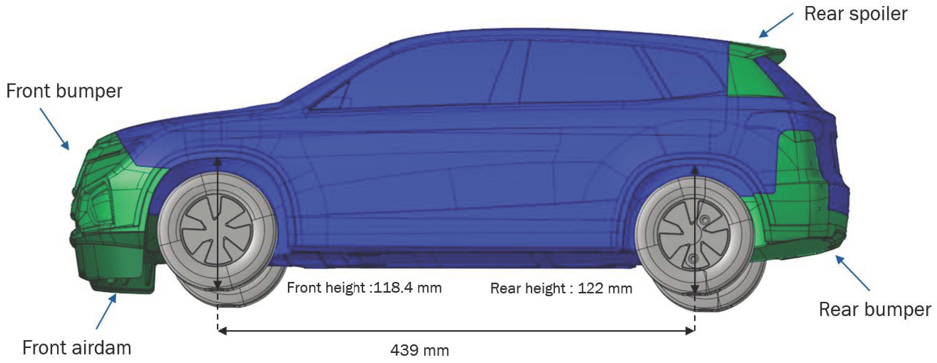
Large flow detachments observed in the rear wake of a Sport Utility Vehicles (SUV) lead to drag values that are much higher than those observed with other vehicle shapes. These flow detachments can be reduced either with rear spoiler inclinations or with underbody shape improvements. Therefore, a modular vehicle mockup provides the testing availability of different geometrical combinations. Figure 1 shows the different modules that can be changed in green. The height of the underfloor can also be modified until reaching the lowest drag value. Front and rear height values are provided for this purpose in the figure below, leading to a drag coefficient Cd of 0.36 for this baseline configuration.
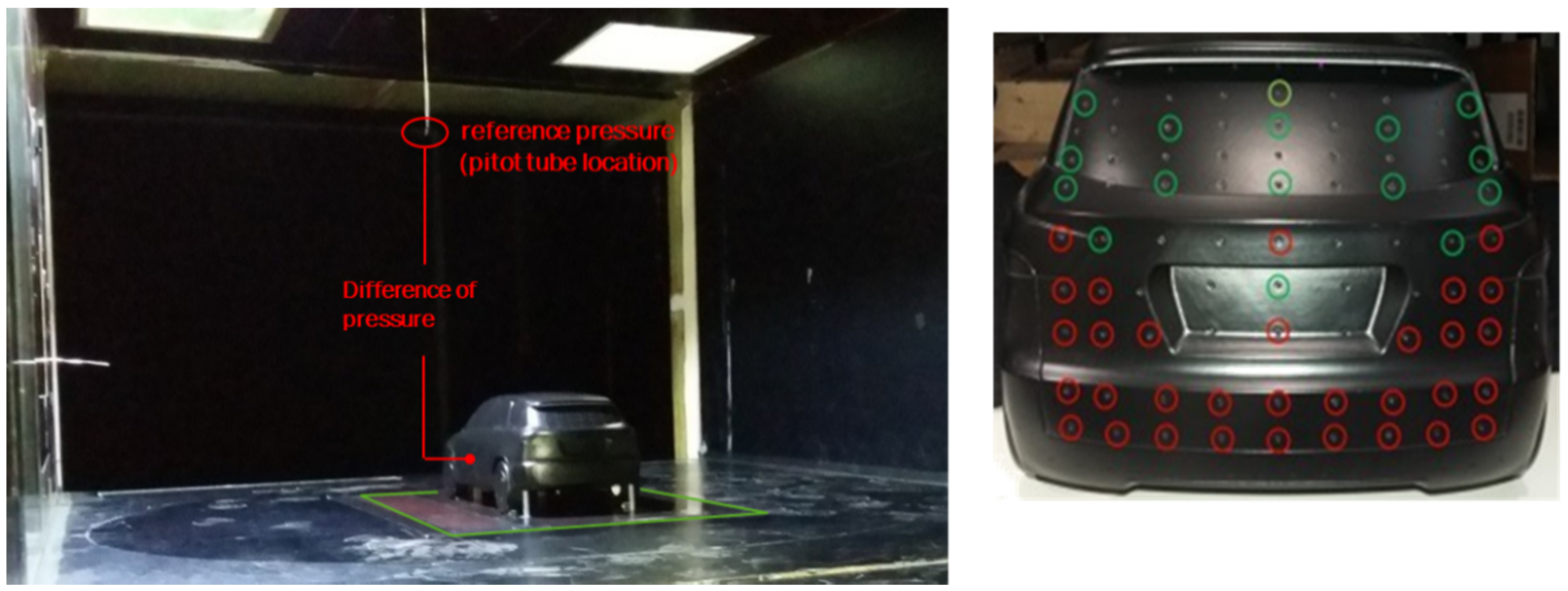
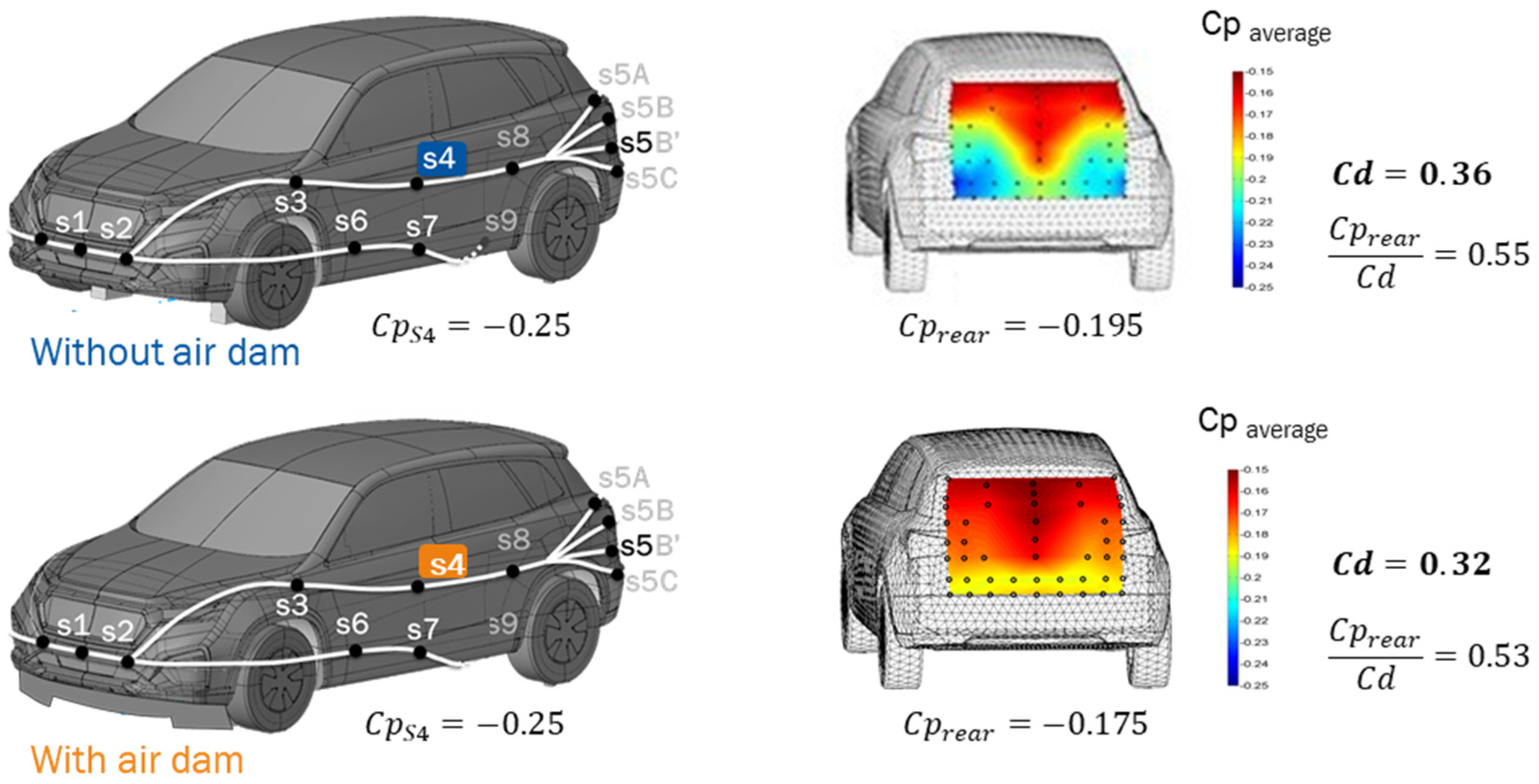
In addition to measurements performed with an aerodynamic balance, 48 pressure sensors mounted at the rear of the mockup enabled the quantification of aerodynamic contributions of the slant window, the tailgate and the rear bumper surfaces. According to the reference pressure taken at the Pitot tube, localized at a height of 1034 mm above the floor and at 630 mm ahead the front bumper (Figure 2), pressure measurements on these three rear surfaces lead to a partial Cd ratio between 55% and 53% with or without an air dam (Figure 3). Therefore, the optimization objective seems to be applicable either on the total Cd or on the rear wall pressure.
Thanks to an experimental design-of-experiment method, it has been found that a specific air dam geometry enables a decrease in drag force by 9%, leading to a Cd value of 0.32 and keeping the rear pressure force ratios at a level of 53% (Figure 3). This optimized configuration is now used with the baseline configuration in order to check the grid convergence of the numerical model before performing the optimization process.
Rear pressure and drag coefficients are defined as follows:
C p r e a r = 1 N 1 N P n P P i t o t 1 2 ρ V P i t o t 2
C d = F x 1 2 ρ A V P i t o t 2
where N denotes the number of rear sensors equal to 48, P n denotes the pressure measured at sensor n, P P i t o t denotes the static pressure measure at the Pitot tube location, V P i t o t 2 denotes the velocity measured from dynamic pressure at the Pitot tube equal to 30 m/s and A is the projected frontal area of the mockup equal to 0.06 m2 for a model scale of 1:7. In addition to the rear pressure sensors, several pressure taps have been introduced on both sides of the mockup in order to capture possible asymmetries of the flow. Pressure measurements were conducted at sensor 4 on the left side in the front door (Figure 3) but also on the opposite side [13], and they both provide equivalent values of C p s i d e = 0.24 without any yaw angle.

2.2. Grid Convergence for Lattice Boltzmann Numerical Model

In a lattice Boltzmann method (LBM), velocity and pressure come from the collision equation [15,16]. The time iteration number must be high enough in order to reach the periodic state checked at the reference Pitot tube location. The time step must be in concordance with the cell size in order to capture the convection phenomena respecting the Courant number condition and the inertial slope of the power density spectrum at some specific points situated in turbulent regions behind detachment zones. A Smagorinsky turbulence model is used in the core region of the fluid and a wall model enables the computation of friction velocity in the three first layers in order to match to the non-dimensional velocity profile in the core region.
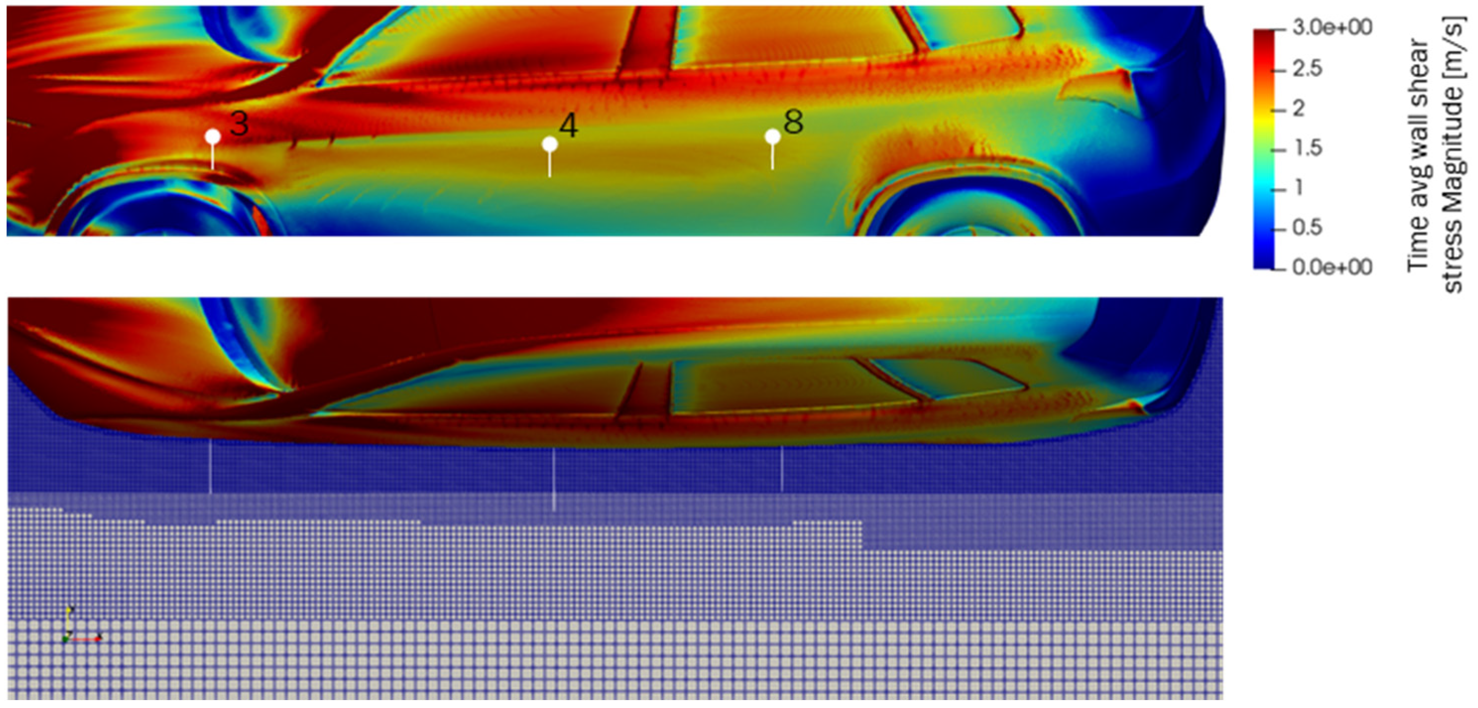
Generally, simulation time for this reduced scale model is set at 2.5 s, and the number of iterations is set at 15,000 for a mesh size of 400 million hexahedron cells or voxels. This numerical model definition enables frequency analysis between 2 Hz and 2500 Hz but needs two and a half days of computation. Therefore, we decrease the simulation time to 1.35 s and the number of iterations to 4000 in order to limit computation time to 4 h for a mesh of 50 million voxels. The cell size in the wall region must also be able to capture the wall friction in the wall model. In this paper, we compare the velocity profiles obtained with the standard fine mesh of 400 million voxels generally used for computations and a coarse mesh of 50 million voxels (Table 1) defined for this optimization study to hotwire measurements at three sensor locations (Figure 4).
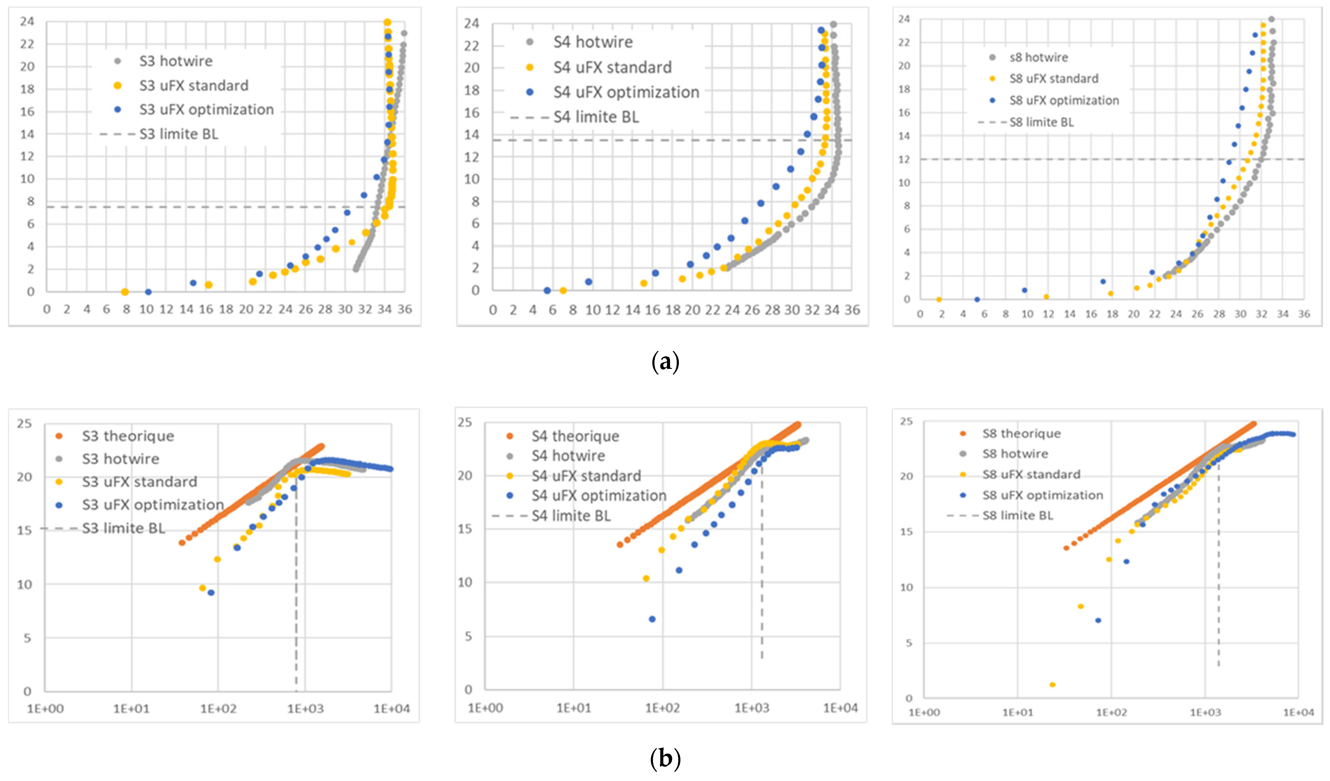
Velocity profiles have been measured thanks to a hotwire system for the baseline configuration, with a step of 0.2 mm starting at 2 mm from the wall. We can notice in Figure 5a that experimental profiles for sensors 4 and 8 (in grey) are very close to the numerical velocity profiles (in yellow) obtained with the reference fine mesh of 400 million voxels (see bottom view of Figure 4). This high number of voxels is due to the size of the five first layers close to the wall, equal to 0.4 mm (see Table 1). Friction velocity U* computed with the fine mesh is equal to 1.7 m/s on sensor 4 and 8 (see top view of Figure 4) and used for reference in order to calculate the non-dimensional velocity profiles U+ such as the following.
U + = f y +   with   U + = U U *   ,   y + = U * y ν   and   ν   the   cinematic   viscosity
Thickness of the boundary layers is estimated at the end of the logarithmic law, which must be parallel to the analytic law (in orange in Figure 5b), and it is defined as follows.
U + = 1 K ln y + + C   with   K = 0.41   and   C = 5
This method enables the ability to find a boundary layer thickness between 12 mm and 14 mm for sensor 4 and 8 (Figure 5a) and avoids questions about velocity acceleration due to the blocking ratio.
Even if the resulting velocity profiles (in blue) on Figure 5a show differences with velocity profiles of the refined mesh (in yellow), slopes in the three first layers lead to the same friction velocity. Differences were observed to be increased at sensor 3 where acceleration of the flow along the fender seems difficult to capture either with coarse or fine mesh. It is, therefore, important to check if the pressure fields in the detachment regions are well computed, especially with coarse mesh in the rear end of the mockup.
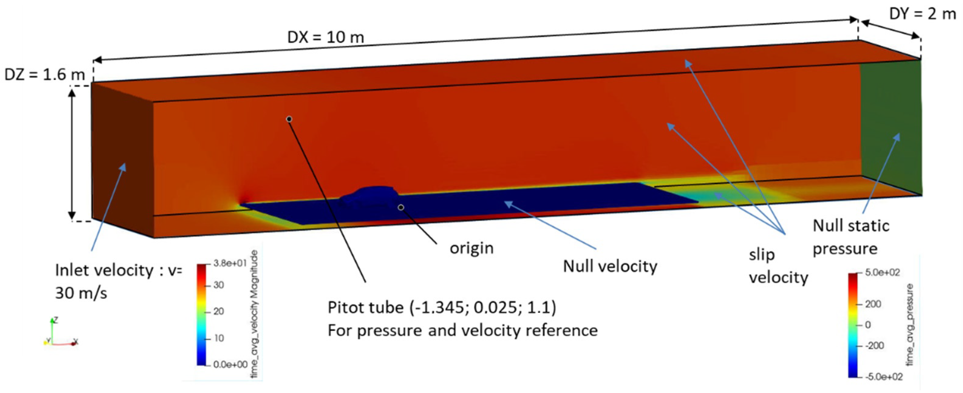
The same velocity profiles have been realized on this baseline configuration with a coarse mesh in order to check if CFD computations are precise enough to create a database in a reasonable time. Voxels measuring 50 million are used in this mesh, with cell sizes of 0.8 mm in the six first layers close to the wall (Table 1). Slip boundary conditions are imposed on the wall of the wind tunnel, and zero velocity conditions are applied on the floor, the wheels and the surfaces of the mockup (Figure 6). An inlet velocity of 30 m/s leads to a velocity at the Pitot tube of 30.6 m/s corresponding to a blocking rate of 1.8%. A zero relative static pressure condition is defined at the outlet. Pressure and drag coefficients are normalized with pressure and velocity magnitudes, measured at the Pitot tube.
According to Figure 7, we obtain a numerical Cd value for this smaller mesh of 0.36 for the baseline and 0.332 for the optimized configurations with pressure map and velocity measurements both averaged on the last 1000 iterations. As a remainder, experimental Cd value is equal to 0.36 in baseline and 0.32 with airdam. These numerical results are in concordance with wind tunnel measurements (see Figure 3).
When taking into account the pressure sensor locations (left side of Figure 7), the rear pressure coefficient versus drag coefficient C p r e a r / C d of the computed baseline configuration is equal to 58%, close to the ratio of 55% found in experiments (Figure 3). When using the slant and tailgate surfaces, this pressure ratio is equal to 30%. This difference of rear pressure ratio found between rear pressure sensors and rear partial surfaces is due to a higher density of the pressure sensors in the region of low-pressure values, especially in the rear bumper region.
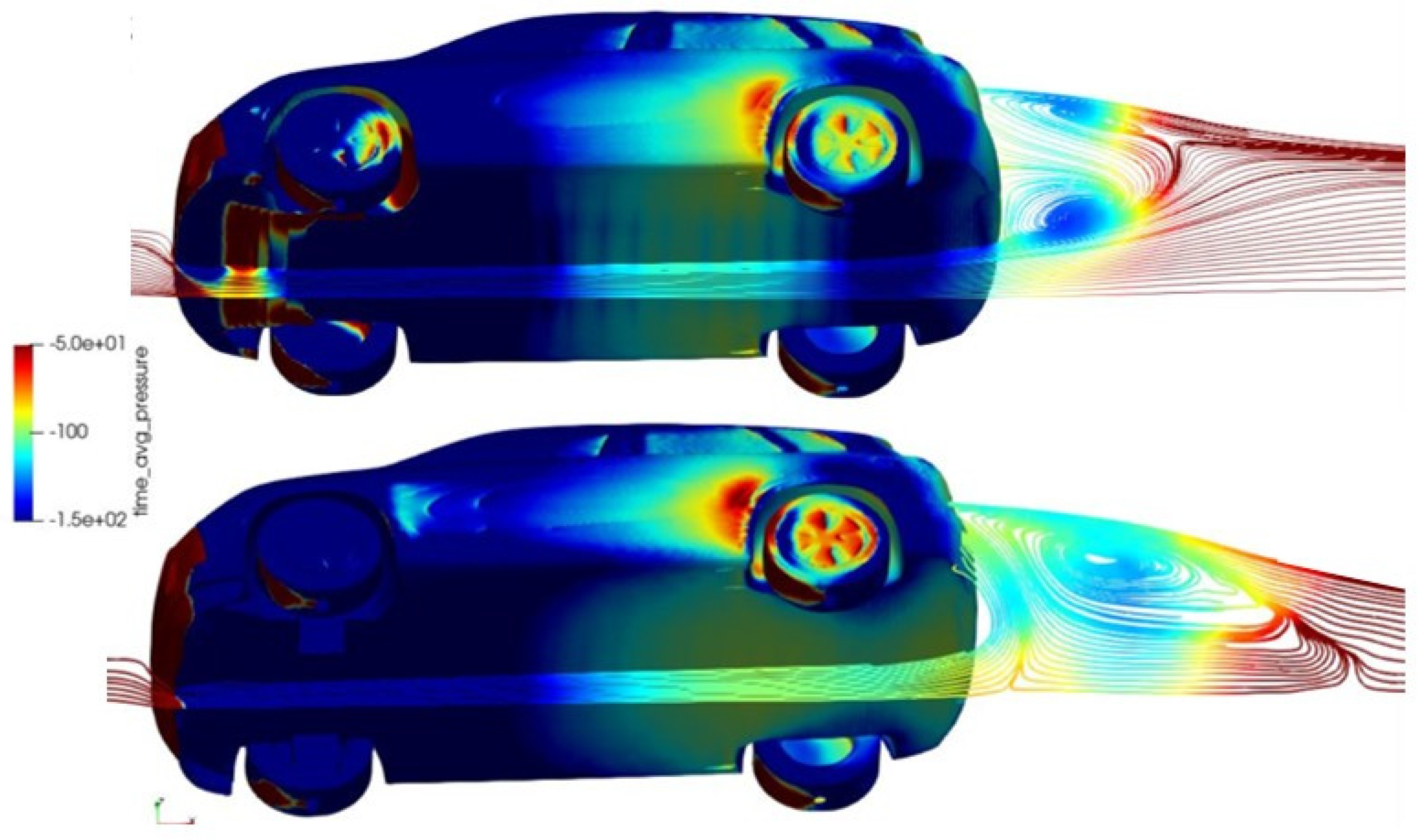
In relation with wall pressure map of Figure 7, streamlines in the symmetry plane in the longitudinal direction show influence of the air dam on wake structure (Figure 8). Without the air dam, airflow in the underfloor creates a recirculation behind the rear bumper. With the reference air dam, this bottom recirculation disappears, increasing the size of the remaining recirculation, which pushed itself downward. Pressure in the wake increases, leading to drag force reduction in the tailgate. However, this benefit is balanced by an increase in pressure on the front air dam. Nevertheless, numerical Cd reduction is equal to 8% compared to an experimental gain of 9%.
Thanks to the numerical model’s definition, computation takes 4 h on a DGX-1 machine working with 8 GPU Tesla cards of 32 GByte of RAM per card for a numerical model of 50 million voxels. Depending on the number of free variables, this solver time per variant leads to a total computation time of one month in order to build up the database for the surrogate by running the design-of-experiments.

2.3. Shape Optimisation Process

According to the optimized configuration described above, there is an air dam geometry decreasing drag forces by 8% (Figure 6). However, the absolute total height of this geometry limits its integration below the front bumper due to the style issues and the reliability of the system. A design exploration of the geometric parameters must help delivering a less intrusive shape with similar aerodynamic performance.
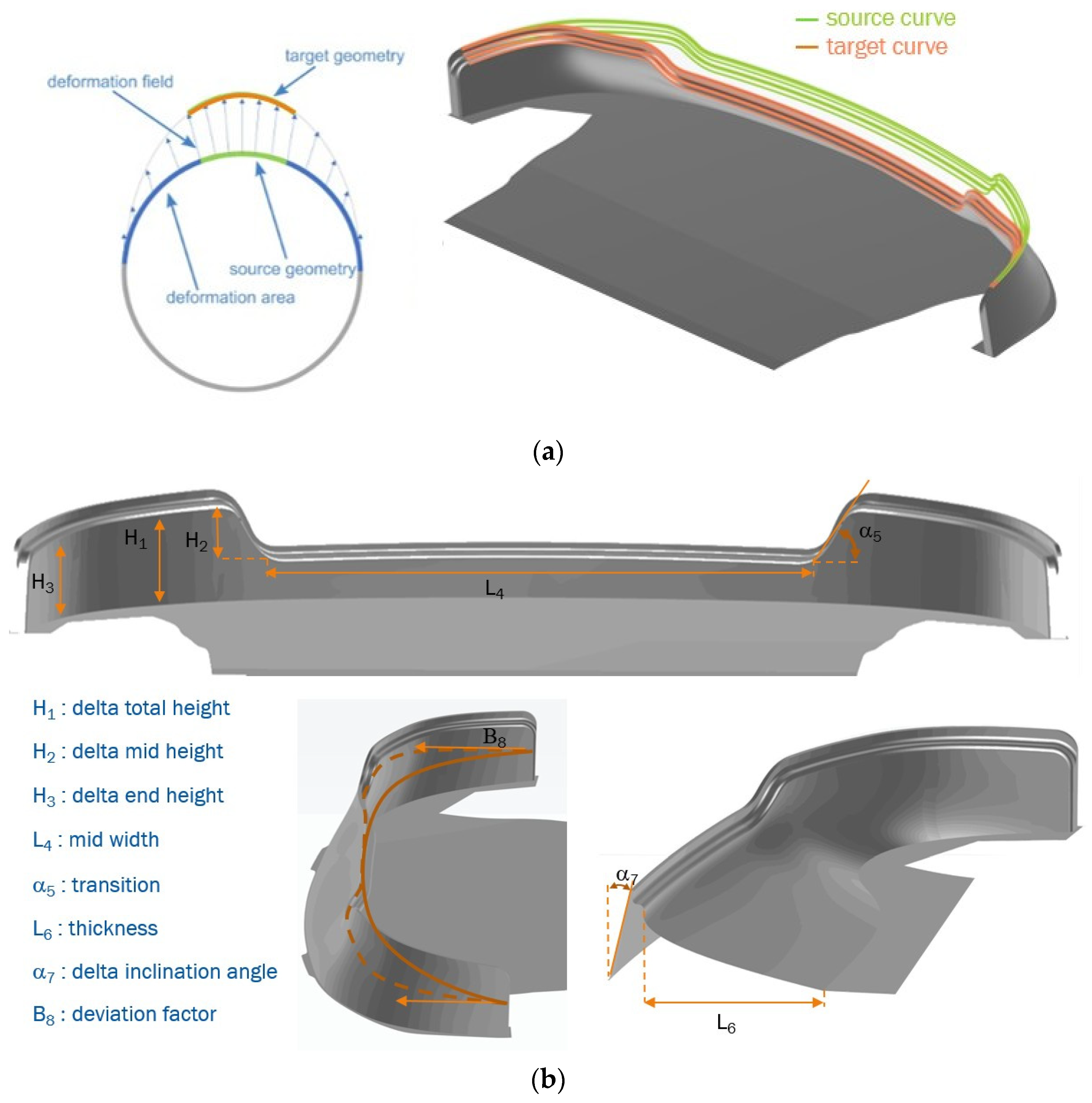
Starting from the most efficient air dam geometry, Radial Basis Functions (RBFs) are applied on the source curves in order to deform the shape until reaching the target curves. Target curves, defined as NURBS, are morphed with their control points, according to geometric parameters such as the total height of the air dam and the height and the width of the central section. Figure 9a shows a description of the deformation process, and Figure 9b presents the eight geometric parameters retained to morph the shape of the air dam.
The new air dam geometry is exported in the STL format and joined to the static STL file of the numerical model. The volume hexahedral mesh, performed in the closed volume limited by the shell mesh, enables the computation of a new aerodynamic solution thanks to the lattice Boltzmann method with the cell size definition selected from the grid convergence study.
There are different methods for building response surfaces (surrogates) used to search a minimum number of objective functions. The Latin Hypercube technique is often used, but Sobol sequence is preferred as this global sensitivity analysis method based on variance decomposition enables adapting sampling during design space exploration. The precision of the resulting surrogate model can be increased thanks to additional sampling, dealing with extended geometric parameter ranges [17].
As mentioned in the Introduction, response variables have been chosen in order to explore numerical solutions close to the experimental results. The objective is the drag value and constraints dealing with pressure sensor values on the side and at the rear of the mockup. Sampling results must show the response surface of the minimum drag value in the range of pressure constraints. Figure 10 illustrates the process with objectives and constraints definition. An error of Cd corresponds to the difference between a computed Cd value and the objective value of 0.32. An error of 0.02 corresponds then to a Cd of 0.34. Therefore, an error on Cpside4 of 4 will correspond to a value of −0.21 and an error on C p r e a r / C d of 0.1 corresponds to a value of 0.25. Results of the Sobol sequence are presented in the next section.
Surrogate models are often built from the available design space database, either with artificial neural networks or with a Kriging model. This model, also called a Gaussian process, enables the prediction of the objective of function f(x) depending on the range of the geometric variable vector dataset x _ thanks to the following relation:
f ^ g x _ T β _ + r _ x _ ¯ T R _ ¯ 1 f _ G _ ¯   β _
with x _ being the vector of design variables of dimension n, g _ ( x _ ) is the vector of trend basis functions, β _ is a vector containing the generalized least squares estimates of the trend basis function coefficients, r _ ( x _ ) is the correlation vector of terms between x and the data points, R _ ¯ is the correlation matrix for all of the data points, f _ is the vector of response values and G _ ¯ is the matrix containing the trend basis functions evaluated at all data points. Correlation vector r _ ( x _ ) and matrix R _ ¯ are computed using a Gaussian correlation function depending on a vector of correlation parameters of dimension n, θ _ = {θ1, …, θn}T using a Maximum Likelihood Estimation (MLE) procedure involving the Likelihood join probability function p(y|θ). Therefore, the Kriging model allows an approximation of predictors and their uncertainty through the mean square error (MSE). The Kriging model defined and used in this paper has been introduced in Dakota, an optimization algorithm available from the Sandia National laboratory [18] and implemented in CAESES©.
This CFD optimization study deals with drag coefficient reduction with pressure constraints. Therefore, we need to solve a multi-objective problem in order to find the global minimum of the individual objective functions defined thanks to each Kriging model: m i n f 1 x _ , f 2 x _ , f m x _ with m corresponding to the number of objectives. As CFD simulations can lead to different minimums according to flow topology change, a multi-objective genetic algorithm (MOGA) seems to be the most appropriate in order to find the global minimum in the objective space. This genetic algorithm uses a two-point crossover technique, starting from 50 random design points. The result is a population of the 10 best “parent” (elitist strategy) plus 40 new “children”. The MOGA optimization process is finished after either 150 generations or 2000 function evaluations. We will then be able to select the minimum drag objective value in the response surface that is associated with pressure objective values.
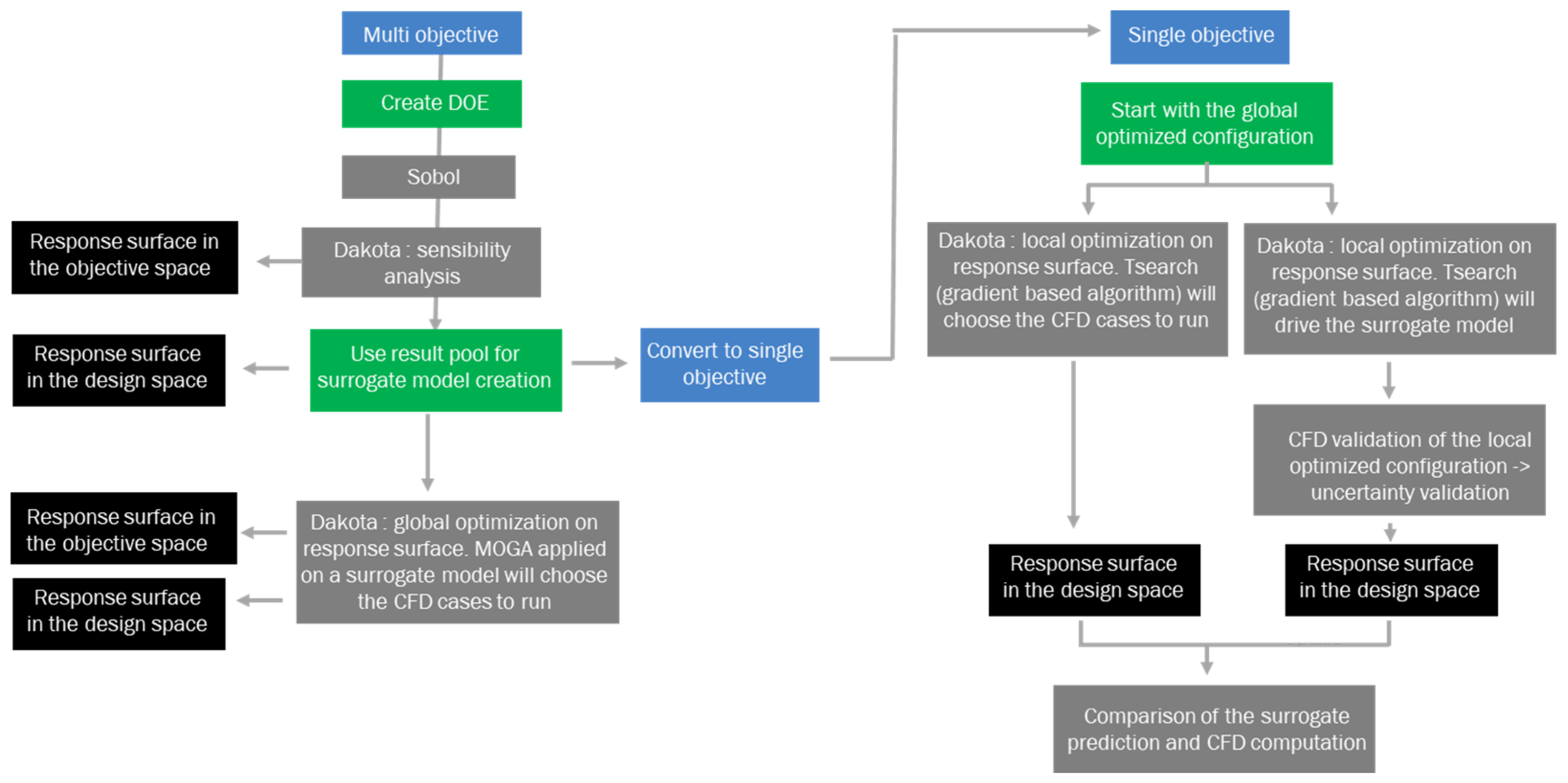
Due to pressure constraints, the minimum value of the drag coefficient may be decreased, performing a single-objective optimization in the design space. This second optimization process can involve a genetic algorithm on the single function of the Kriging model or a gradient search (Tsearch algorithm) applied on the surrogated model and verified with CFD computations. A gradient search on the surrogate model could help in understanding the relation between design variables and drag values. Then, CFD computations performed at specific points enables the verification of whether the resulting CFD-computed Cd values are close to the Kriging model’s prediction. In cases where CFD results are far from the Kriging prediction, a gradient search can be performed using CFD computations directly without surrogate models. Figure 11 presents these different possibilities.
3. Results

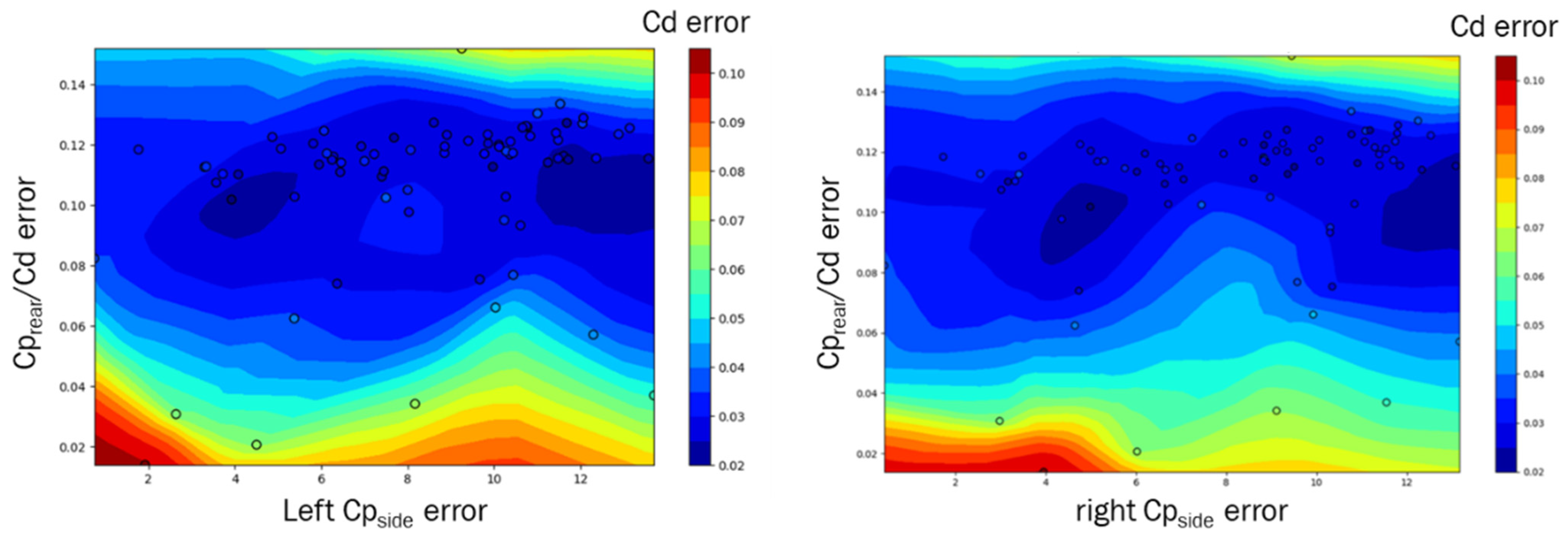
Thanks to the optimization process described in Section 2.3, we focus first on the response surface in the objective space, obtained at the end of the Sobol sequence after 80 sample computations. Figure 12 shows the Cd values versus the rear pressure ratio and the side pressure values situated on the front doors (on the left for the driver side and on the right for the passenger side). Both figures show that Cd error is at the minimum and equal to 0.02, meaning that Cd = 0.34 when the error side pressure is close to 4 from the conditions given in Figure 10, which means that C p s i d e = 0.21 instead of the expect value of −0.25. This minimum Cd value of 0.34 is related to an error of the rear pressure ratio equal to 0.10, which means that C p r e a r / C d = 0.25, a ratio smaller than the expected value of 0.30 given in Figure 7.
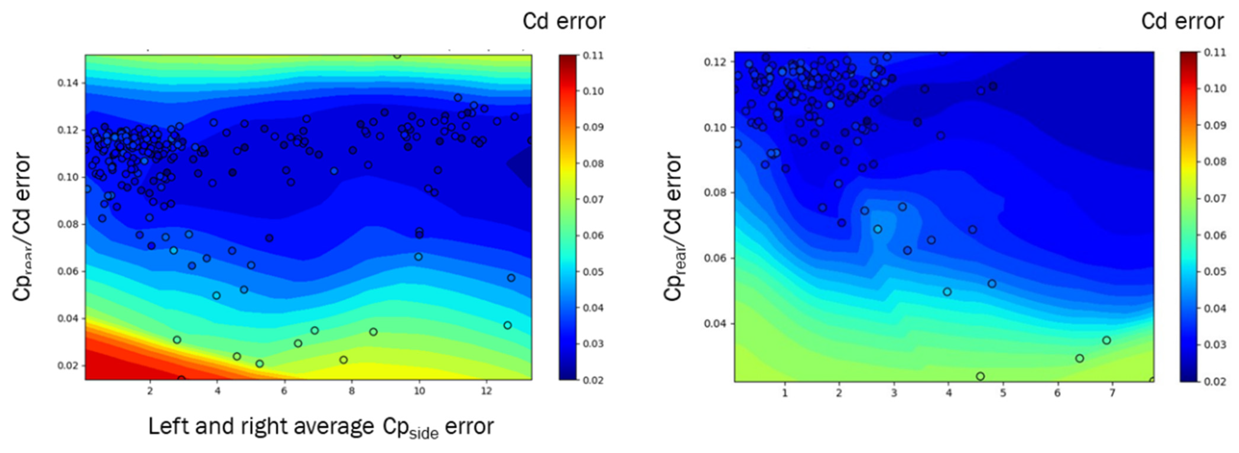
This Sobol sequence database helps in creating the Kriging model used to optimize the drag objective under pressure constraints. Figure 13 shows that the MOGA algorithm, available in CAESES© via the embedded Dakota optimization kit, finds a minimum Cd error of 0.02 for a minimum side pressure error close to zero but with a minimum error on the rear pressure ratio above 6%. It means that the best Cd reductions found in this current database are related to a decrease in the rear pressure contribution and inversely to an increase in air dam dam contribution. The constraint applied on the C p r e a r / C d ratio seems, therefore, difficult to respect completely, meaning that the best aerodynamic performances are obtained with airdam designs inducing important pressure forces. Nevertheless, additional samples selected with the MOGA technique must lead to the aerodynamic performances of airdam geometry presented in Figure 7.
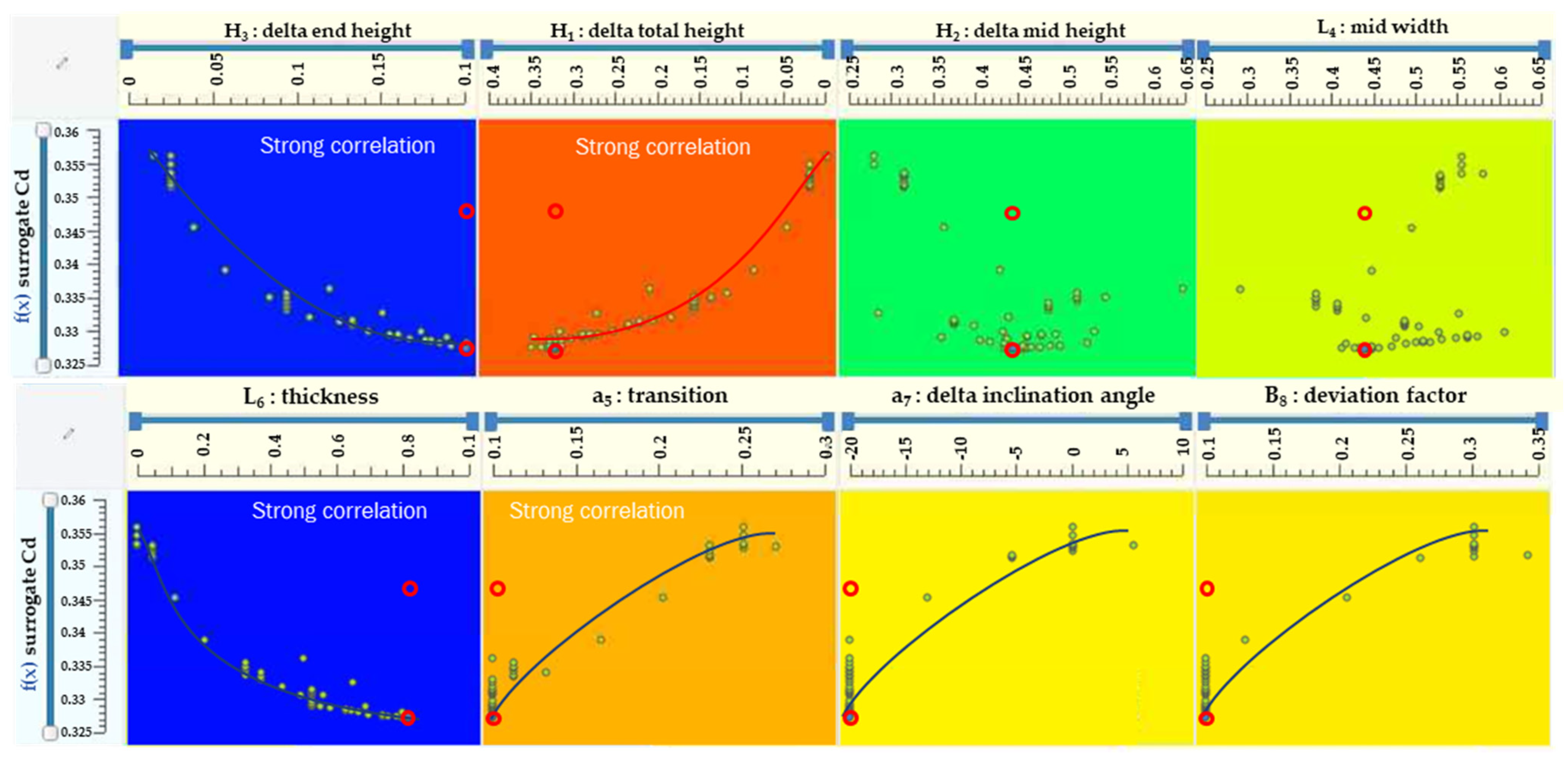
A gradient-based optimization technique is then performed based on the Kriging model of the drag coefficient objective in order to test its prediction uncertainty. Analysis of the Pareto curves deals with Cd variation for each design parameter. Figure 14 shows that strong correlations are found for four design parameters (delta_end_height, delta_total_height, thickness and transition), leading to the minimum value of Cd = 0.327, which is better than the optimized value of 0.332 presented in Figure 7. However, CFD validation for this design provides Cd = 0.348. This validation result far from expectation shows that the surrogate model must be completed with additional computed samples, including this final computation result. An iterative process involving predictions and CFD computations will help find the missing samples leading to an increase in the coefficient of determination R2, defined as the proportion of the predictable variations of the design variables and computed thanks to Maximum Likelihood Estimation (see Section 2.3).
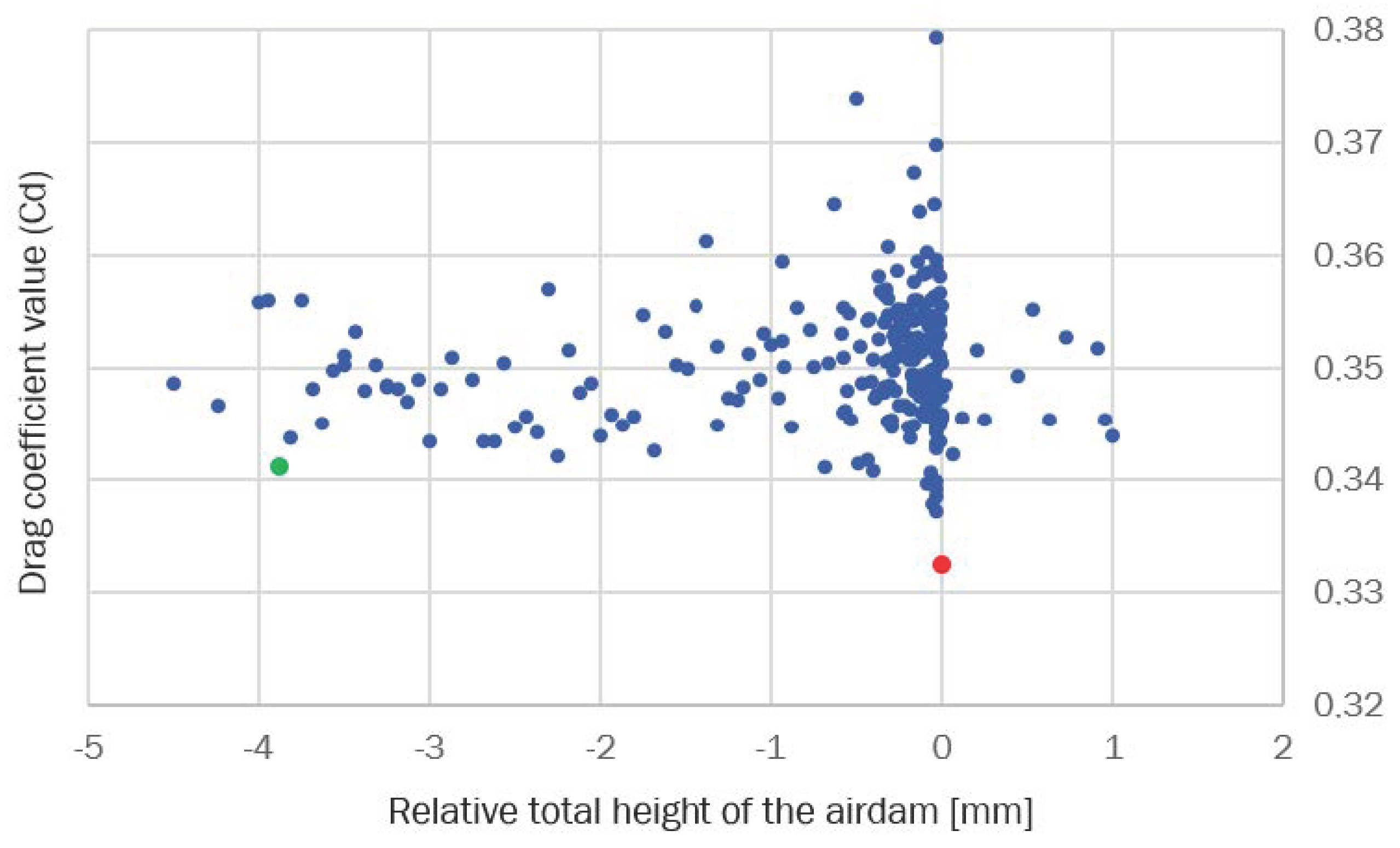
Even though the optimization process cannot reach any Cd value below the reference air dam value of 0.332, a second important objective is to decreasing the maximum height of the air dam for style and system reliability purposes. According to the available CFD database composed of 230 Sobol and Dakota configurations, we focus now on the air dam’s minimum height, which is related to a local minimum of the drag coefficient values (Figure 15). Compared to the reference air dam configuration in red, there exists a local optimized configuration in green, decreasing the air dam height of 16% for a Cd increase of 2.6%. In addition to the total height reduction, the small height in the middle section (right view of Figure 16) has great advantages for product reliability. The pressure force will be lower and torque actuation smaller in cases of air dam deployment. A numerical Cd reduction limited to 5%, compared to the potential maximum Cd reduction of 8%, still remains interesting.

4. Conclusions

Aerodynamic optimization with shape deformation is a research domain involving many topics. Surrogate models such as Artificial Neural Networks and Kriging models become popular and can be utilized in connection with different CFD solvers. Surface morphing with Radial Basis Functions (RBFs) are now well known, and techniques for DoE sampling can easily be introduced in simulation processes. Gradient or genetic algorithm methods also gain popularity for aerodynamic optimization purposes. It seems, therefore, reasonable to create CFD databases dealing with design exploration for aerodynamic project optimization without expending too much effort.
Most CFDs or wind tunnel databases are created thanks to discrete parameters. It misses some optimization example feedback dealing with morphing. Optimization analysis in this paper shows some potential difficulties in order to create surrogate models correlating precisely design parameters with aerodynamic objectives. DoE sampling is, therefore, an important step in order to constitute response surfaces leading to reliable Pareto curves and precise objective predictions. The sampling size of DoE is crucial: If it is too large, the time and resources spent on simulations are prohibitive; if it is too small, the quality of the predicted vs. the computed results is insufficient. There are methods for placing additional simulations strategically, namely where the error between actual results from CFD and predicted results from the surrogate are considerable and/or where very beneficial designs are likely to occur.
In this study, we can also observe that multi-objective optimization with pressure constraints could help in understanding issues in the comparison method between numerical and experimental results. Side pressure constraints are easy to respect but the averaging process for rear pressure calculation needs to be precisely defined.
Physical analysis of the CFD database created thanks to the Sobol sequence shows some local minimum, which might be interesting for air dam shape definition. Drag reduction remains at a high level for significant product design advantages.

Author Contributions

Conceptualization, P.G. and S.H.; methodology, C.E., P.G. and S.H.; software, C.E. and P.G.; validation, C.E. and P.G.; formal analysis, C.E. and P.G.; investigation, C.E., Y.E., P.G. and C.N.N.; resources, C.E., P.G., S.H. and C.N.N.; data curation, C.E., Y.E. and P.G.; writing—original draft preparation, P.G. and S.H.; writing—review and editing, P.G.; visualization, C.E., Y.E. and P.G.; project administration, P.G. All authors have read and agreed to the published version of the manuscript.

Funding

This research received no external funding.

Data Availability Statement

Data belong to the authors and are not public. Please contact the authors for more information’s.

Acknowledgments

This CFD optimization process has been performed involving ultraFluidX©, a lattice Boltzmann solver developed by Altair®. We would like to thank and acknowledge Altair® for their support in finding issues in coupling ultraFluidX© version 2020 to CAESES© version 5.11.

Conflicts of Interest

The authors declare no conflict of interest.

References

  1. Eulalie, Y.; Fournier, E.; Gilotte, P.; Holst, D.; Johnson, S.; Nayeri, C.N.; Schütz, T.; Wieser, D. Active flow control analysis at the rear of an SUV. Int. J. Numer. Methods Heat Fluid Flow 2018, 28, 1169–1186. [Google Scholar] [CrossRef]
  2. Karpouzas, G.K.; Papoutsis-Kiachagias, E.M.; Schumacher, T.; De Villiers, E.; Giannakoglou, K.C.; Othmer, C. Adjoint Optimization for Vehicle External Aerodynamics. Int. J. Automot. Eng. 2016, 7, 1–7. [Google Scholar] [CrossRef] [Green Version]
  3. Othmer, C. Adjoint methods for car aerodynamics. J. Math. Ind. 2014, 4, 6. [Google Scholar] [CrossRef] [Green Version]
  4. Harries, S.; Abt, C. Faster Turn-around Times for the Design and Optimization of Functional Surfaces. Ocean Eng. 2019, 193, 106470. [Google Scholar] [CrossRef]
  5. Albert, S.; Hildebrandt, T.; Harries, S.; Bergmann, E.; Kovacic, M. Parametric Modeling and Hydrodynamic Optimization of an Electric Catamaran Ferry based on Radial Basis Functions for an Intuitive Set-up. In Proceedings of the Conference on Computer Applications and Information Technology in the Maritime Industries (COMPIT 2021), Mühlheim an der Ruhr, Germany, 9–10 August 2021; pp. 58–78. Available online: http://data.hiper-conf.info/compit2021_muelheim.pdf (accessed on 7 August 2021).
  6. Harries, S.; Abt, C.; Brenner, M. Upfront CAD—Parametric Modeling Techniques for Shape Optimization. In Advances in Evolutionary and Deterministic Methods for Design, Optimization and Control in Engineering and Sciences; Minisci, E., Vasile, E., Periaux, M., Gauger, J., Giannakoglou, N., Quagliarella, K., Eds.; Springer: Berlin/Heidelberg, Germany, 2018. [Google Scholar] [CrossRef]
  7. Papoutsis-Kiachagias, E.M.; Asouti, V.G.; Giannakoglou, K.C.; Gkagkas, K.; Shimokawa, S.; Itakura, E. Multi-point aerodynamic shape optimization of cars based on continuous adjoint. Struct. Multidiscip. Optim. 2019, 59, 675–694. [Google Scholar] [CrossRef]
  8. Zhou, H.; Ren, C.; Wu, H.; Chen, Q.; Jadhav, T. Multi-Objective Aerodynamic Optimization of Vehicle Shape Using Adjoint Approach Based on Steady-State and Transient Flow Solutions; SAE Technical Paper 2021-01-0945; SAE International: Warrendale, PA, USA, 2021. [Google Scholar] [CrossRef]
  9. Harries, S. Practical Shape Optimization Using CFD: State-Of-The-Art in Industry and Selected Trends. In Proceedings of the Conference on Computer Applications and Information Technology in the Maritime Industries (COMPIT 2020), Pontignano, Italy, 17–19 August 2020; pp. 197–222. Available online: http://data.hiper-conf.info/compit2020_pontignano.pdf (accessed on 9 August 2020).
  10. Vergnault, E.; Sagaut, P. An adjoint-based lattice Boltzmann method for noise control problems. J. Comput. Phys. 2014, 276, 39–61. [Google Scholar] [CrossRef]
  11. Li, J.; Zhang, M.; Martins, J.; Shu, C. Efficient Aerodynamic Shape Optimization with Deep-Learning-Based Geometric Filtering. AIAA J. 2020, 58, 4243–4259. [Google Scholar] [CrossRef]
  12. Simpson, T.W.; Mauery, T.; Korte, J.J.; Mistree, F. Kriging Models for Global Approximation in Simulation-Based Multidisciplinary Design Optimization. AIAA J. 2001, 39, 2233–2241. [Google Scholar] [CrossRef] [Green Version]
  13. Gilotte, P.; Mortazavi, I.; Colon de Carvajal, A.; Edwige, S.; Nayeri, C.N. Aerodynamical characteristics of a reduced scale ground vehicle according to yaw angle variations. Int. J. Numer. Methods Heat Fluid Flow 2021, 32, 1222–1236. [Google Scholar] [CrossRef]
  14. Zhou, Q.; Jiang, P.; Huang, X.; Zhang, F.; Zhou, T. A Multi-objective robust optimization approach based on Gaussian process model. Struct. Multidiscip. Optim. 2018, 57, 213–233. [Google Scholar] [CrossRef]
  15. Malaspinas, O.; Sagaut, P. Consistent subgrid scale modelling for lattice Boltzmann methods. J. Fluid Mech. 2012, 700, 514–542. [Google Scholar] [CrossRef]
  16. Malaspinas, O.; Sagaut, P. Wall model for large-eddy simulation based on the lattice Boltzmann method. J. Comput. Phys. 2014, 275, 25–40. [Google Scholar] [CrossRef]
  17. Wang, P.; Lu, Z.; Tang, Z. An application of the Kriging method in global sensitivity analysis with parameter uncertainty. Appl. Math. Model. 2013, 37, 6543–6555. [Google Scholar] [CrossRef]
  18. Giunta, A.A.; Swiler, L.P.; Brown, S.L.; Eldred, M.S.; Richards, M.D.; Cyr, E.C. The Surfpack Software Library for Surrogate Modeling of Sparse Irregularly Spaced Multidimensional Data. In Proceedings of the 11th AIAA/ISSMO Multidisciplinary Analysis and Optimization Conference, AIAA Paper 2006-7049, Portsmouth, VA, USA, 6–8 September 2006. [Google Scholar] [CrossRef] [Green Version]
Figure 1. Modules in green can be removed from the blue mockup in order to test different variants of the front and rear bumper, front air dam and rear spoiler.
Fluids 07 00166 g001
Figure 2. Mockup mounted in the wind tunnel, with the Pitot tube location. Tailgate and rear bumpers are equipped with instantaneous pressure sensors.
Fluids 07 00166 g002
Figure 3. Rear pressure coefficient with and without air dam. C p r e a r / C d Ratio is around 50% in both configurations in experiments.
Fluids 07 00166 g003
Figure 4. Wall shear stress computed with the most refined grille at Z = 140 mm (bottom view). The friction velocity values (top view) are used to compute non-dimensional velocity profiles.
Fluids 07 00166 g004
Figure 5. (a) Velocity profiles at different locations (on the fender for sensor 3, below the front window for sensor 4 and below the rear window for sensor 8) thanks to hotwire measurements in grey, with a fine mesh in yellow and with a coarse mesh in blue. (b) Experimental and numerical non-dimensional velocity profiles at different locations. End of the logarithmic law correspond to the end of the boundary layer. uFX Standard corresponds to the fine mesh and uFX optimization to the coarse mesh. The theorique profiles are computed thanks to Equation (4).
Fluids 07 00166 g005
Figure 6. Description of the boundary conditions used for CFD computations.
Fluids 07 00166 g006
Figure 7. Rear pressure on the last 1000 iterations for the baseline and optimized air dam CFD configuration, respectively, equal to 0.360 and 0.332. Drag coefficient gain is close to 8%. Numerical C p r e a r / C d ratio is equal to 58% when taking pressure taps and close to the ratio of 55% found in measurements. Meanwhile, pressure ratio of the slant and the tailgate surfaces is equal to 30%.
Fluids 07 00166 g007
Figure 8. Streamlines in the middle longitudinal section colored by the pressure field. Existing recirculation without air dam (top view) behind the rear bumper disappears with air dam (bottom view).
Fluids 07 00166 g008
Figure 9. (a) Source and target NURBS defined with radius basis functions. The source curve in green corresponds to an absolute total height of the air dam of 280 mm. (b) Definition of the design parameters related to the control points.
Fluids 07 00166 g009
Figure 10. Design space exploration with Sobol sequence of the morphed air dam geometry, with objective and constraints values.
Fluids 07 00166 g010
Figure 11. Different optimization methods used for drag reduction with (left) and without (right) pressure constraints.
Fluids 07 00166 g011
Figure 12. Cd objective versus rear pressure ratio and side pressure values for the driver side on left and passage side on right.
Fluids 07 00166 g012
Figure 13. Cd objective versus rear pressure ratio and side pressure value for the Sobol and Dakota in left and Dakota only on the right.
Fluids 07 00166 g013
Figure 14. Cd objective curve versus design variables obtained with a gradient search on the Kriging model. The red circle at Cd = 0.348 corresponds to CFD validation with regard to the optimized predicted Cd value of 0.327.
Fluids 07 00166 g014
Figure 15. Cd objective versus the total height of the air dam. Red point corresponds to the reference air dam configuration (not practical for reasons of style and reliability), green point to the minimum air dam height geometry (acceptable without too heavy losses in performance).
Fluids 07 00166 g015
Figure 16. Air dam geometry for the reference case (left view) measured in the wind tunnel and the local optimized case (right view) with a reduced total height.
Fluids 07 00166 g016
Table 1. Boundary layer definition for the mesh of 50 million voxels and 400 million voxels according to their voxel refinement (Vr) distribution.
Vr NumberCell Size per Vr [mm]nb of Layer per VrThickness [mm]
(50 million voxels)
70.7812564.69
61.56251218.75
53.125618.75
46.25850
(400 million voxels)
70.39062551.95
60.781252721.09
51.56251117.19
43.1251650
Publisher’s Note: MDPI stays neutral with regard to jurisdictional claims in published maps and institutional affiliations.