Abstract
In the current paper, a new formula for calculating boundary layer quantities—such as the boundary layer thickness, friction coefficients, and the boundary layer profile—for a flat plate is presented. The formula is based on the power-law approach and represents a generalisation of the 1/7 power-law to a more extensive Reynolds number range. In addition to the derivation and the theoretical background, the main focus is on the comparison with various experimental data from the literature. The good agreement of the data shows that this approach allows for precise predictions of boundary layer quantities for a flat plate with zero-pressure gradients. Especially for estimating boundary layers along with large vehicles such as trains, ships, or aeroplanes, the formula offers added value in terms of accuracy compared to previously existing approaches, such as the 1/7 power-law.
1. Introduction
Even though, currently, the determination of boundary layer quantities by means of empirical or semi-empirical formulae is not as important as it was a few decades ago due to the possibilities offered by numerical simulations, there are many applications where such formulae are used. Examples are the correct dimension of experimental or numerical setups and validation of their results. Especially in applications where the development of the boundary layer is crucial for the flow pattern, a formula-based estimation of the boundary layer quantities is essential for the design of experimental and numerical simulations and scaling of the results (e.g., the flow around roof elements on trains [1] or at the rear of a vehicle and the associated effect on the slipstream [2]).
Currently, the so-called 1/7 power law is usually used for such analyses [3]. However, especially for vehicles where the vehicle length and speed result in very high Reynolds numbers (with being the fluid’s kinematic viscosity), significant deviations of the measured boundary layer parameters from those calculated with the 1/7 power-law can be observed [4]. In the past, this was mainly attributed to 3D effects or flow detachment at the rather blunt vehicle shapes but can also be observed for today’s aerodynamically optimized high-speed trains. As shown in [4], a much better agreement is achieved when a power-law with is used, where the value of depends on the Reynolds number . Although this finding is by no means new [5], it is still little or not at all taken into account in vehicle aerodynamics.
One reason for this could be that even for the simple case of a flow over a flat plate, at first glance—more than 100 years after the introduction of Prandtl’s approaches to boundary layer theory—there is no agreement on how this flow can be correctly approximated. In recent decades, there have been heated debates about utilising a power-law or logarithmic approach [6,7].
The power approach describes the relationship of the dimensionless boundary layer quantities and as follows:
with empiric constants and , whereby in the formulation
with empirical quantities and is used. Here, represents the near-wall velocity normalised with the shear stress velocity :
and the dimensionless wall distance:
is the local velocity, the distance to the wall, and is defined as
with wall shear stress and fluid density . All quantities considered are averaged over time.
With the logarithmic approach, the relationship between u+ and y+ is
with and being determined empirically. It seems certain that both approaches cannot be considered as independent of the Reynolds number [6,8]. As an example, in Figure 1, and are plotted over the Reynolds number , where represents the momentum thickness (often also referred to as ).
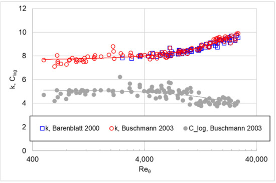
Figure 1.
Power-law parameter and logarithmic law parameter plotted over the Reynolds number with corresponding linear fit (solid lines), according to the data provided by Barenblatt et al. [9] and Buschmann and Gad-el-Hak [6].
The present work does not aim to settle the debate about a correct approach. However, since the power-law approach seems to cover the boundary layer profile in the outer layer somewhat better than the logarithmic approach [6], this approach will be used in the following to derive a new formula for determining boundary layer quantities.
In [4], the formulae for the boundary layer thicknesses (often referred to as ), , (or ) and the friction coefficient were derived using the power-law approach as a function of and . In the present paper, the relationship of and to the Reynolds number, as given in the literature, is to be used directly to obtain a formula for the boundary layer quantities that depends exclusively on the Reynolds number. This corresponds to an extension of the validity of the 1/7 power-law to a more comprehensive range of Reynolds numbers. Subsequently, the results are compared with experimental data available from the literature.
2. Method
In [6,9], and values are presented, which were determined independently based on different experimental data, but mainly on those of Österlund [10]. As shown in [6,11], the profiles of flat plate flow and pipe flow differ, so only the values determined for a flat plate with zero-pressure gradients will be used in this study. As can be seen in Figure 1, there is good agreement between the results determined by [6,9]. These results are used for the following analysis.
To reduce the influence of the laminar-turbulent transition or other upstream effects, boundary layer analyses are usually based on the Reynolds number , which refers to the momentum thickness. However, such an approach is not suitable for predicting boundary layer quantities since the momentum thickness is unknown in the first place. Therefore, for practical reasons, the Reynolds number is used as a reference in the following. Besides, as shown in [12], the relationship between and is similar for most data (see also Section 3.1). Furthermore, the investigations by Marusic [13] have shown that for perfect comparability of measurement data, the use of is also not sufficient, since, for example, the transition itself (e.g., type of tripping tape) also influences the development of the turbulent boundary layer. However, such effects cannot and should not be considered here.
For the and values given by [6,9], the relation , determined from Österlund’s data [10], applies. Based on this, the following applies for and :
These relations now shall be used to calculate the boundary layer quantities only depending on the Reynolds number. The flow profile within the boundary layer follows from Equations (2)–(4)
and for the transition of boundary layer flow to the undisturbed flow
Dividing Equation (9) by (10) leads to the well-known boundary layer profile
The displacement thickness and momentum thickness can be derived from conservation laws. Using Equation (11) gives
The wall shear stress is related to by
Combined with the relation from Equation (5), the boundary layer thickness can now be calculated by
with
Using Equations (15)–(17) this leads to
The local friction coefficient then is calculated by
The frictional drag coefficient results from integrating the local friction coefficient over the plate length :
According to Equations (16) and (20) this gives
To replace and , the boundary layer quantities are expressed as
and
For , for example, this gives
and
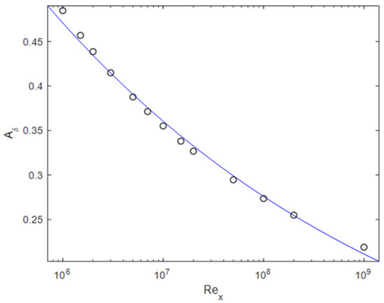
Figure 2.
over according to Equations (7), (8), and (26) (circles) and logarithmic fit (blue line).
Substituting this into Equation (24) then yields
All other quantities can be determined in the same way.
3. Results and Discussion
With the approach presented, the following boundary layer equations can be determined. In the following, the equations presented in Table 1 are compared with experimental data. Only data for (approximately) zero-pressure-gradient flat plate boundary layers determined with appropriate measurement techniques (hotwire, laser Doppler velocimetry) were selected for comparison. Comparable data from direct numerical simulations at corresponding Reynolds numbers are unknown to the author.

Table 1.
Boundary layer formulae.
3.1. Boundary Layer Thickness
Figure 3 compares the formulae given in Table 1 to the experimental data for the boundary layer thicknesses , , and , and the form parameter . Unsurprisingly, the best agreement results for the data are found in the work of Österlund [10], since the values and result from these data. In [10], is calculated instead of , which is why the data are excluded from the comparison. The 1/n power-law seems to better fit the experimental data than the 1/7 power-law. Nevertheless, a final evaluation is difficult because the experimental data show large deviations in the boundary layer thicknesses. Relatively good comparability of the experimental data exists for the shape parameter , which is clearly better represented by the 1/n power-law than by the 1/7 power-law, but still underestimates the experimental results by about 5–7%. The strong deviation of the data from Oweis et al. [14] could result from the pressure gradient present in the experiments.
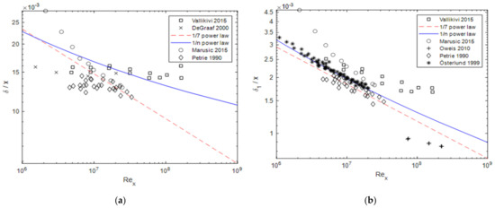
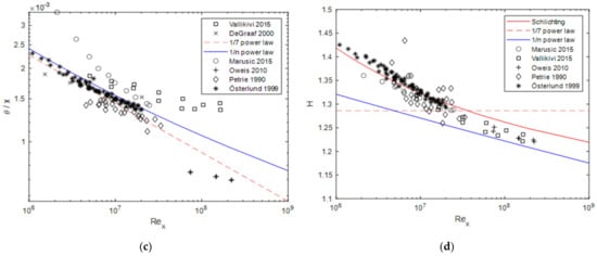
Figure 3.
Boundary layer thicknesses and form parameter compared to the data given by DeGraaff and Eaton [15], Marusic et al. [13], Oweis et al. [14], Österlund [10], Petrie et al. [16], Schlichting and Gersten [17], and Vallikivi et al. [11]: (a) boundary layer thickness; (b) displacement thickness; (c) momentum thickness; (d) form parameter, with Schlichtings formula .
Based on the results for , is plotted against in Figure 4. A good agreement can be found for both the 1/7 power-law and the 1/n power-law. As an example, is also plotted over . It can be seen that this does not result in an improved agreement of the data compared to Figure 3c.
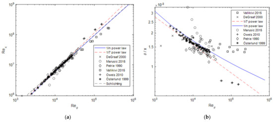
Figure 4.
(a) Reynolds number based on x plotted over the Reynolds number based on ; (b) momentum thickness from different experiments and formulae plotted over .
3.2. Friction Coefficients
Figure 5 compares the local friction coefficient and the friction drag coefficient with experimental data and formulae from the literature. The 1/n power-law is more in line with the experimental results than the 1/7 power-law at high Reynolds numbers. For very low Reynolds numbers, the reference data are slightly exceeded by the 1/n approach. Among other things, this could be because the interpolated values for intercept and slope (cf. Equation (24)) do not quite match the actual values for small Reynolds numbers (see Figure 2). The sensitivity of the results towards slight deviations of the exponent is shown in Figure 5 for the friction coefficient . The Prandtl Schlichting formula [4,17] is usually expressed as
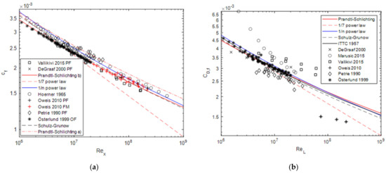
Figure 5.
(a) Local friction coefficient compared to experimental data (as above, but additionally from Hoerner [18]) and the Prandtl–Schlichting formula, as well as the formula given by Schulz–Grunow [19], PF = profile fit, FM = force measurement, OF = oil-film measurement; (b) Friction drag coefficient calculated by , as well as according to [19], according to [17] and according to [20].
Which is shown in Figure 5 as “Prandtl Schlichting (a)”. The correct representation would be “Prandtl Schlichting (b)”:
While the difference in the exponent is only about 1.5%, the resulting values differ by almost 10%.
3.3. Boundary Layer Profiles
Finally, the boundary layer profiles at different Reynolds numbers are compared with selected experimental data. First, the data from Österlund [10] are considered, as these data were used as the basis for and . As shown in Figure 6, the measured profiles agree better with the 1/n power-law than with the 1/7 power-law at higher Reynolds numbers. Compared to the log law, the 1/n power-law seems to give better results further away from the wall, but it is inferior in close wall proximity.
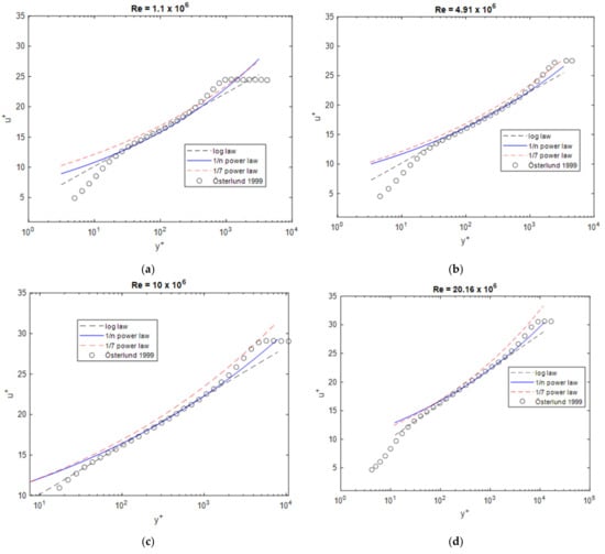
Figure 6.
Boundary layer profiles at different Reynolds numbers compared to the data from Österlund [10], (a) Re = 1.1 × 10⁶, (b) Re = 4.91 × 10⁶, (c) Re = 10 × 106, (d) Re = 20.16 × 10⁶.
Figure 7 compares the results with the data obtained by Marusic et al. [13], one of the most recent studies, which are in a similar Reynolds number range to Österlund’s experiments [10]. The observations are the same as in Figure 6. Interestingly, there is good agreement between the profiles by Österlund and Marusic determined at the same Reynolds number (Figure 7d), while the derived boundary layer quantities in Figure 3 show significant differences.
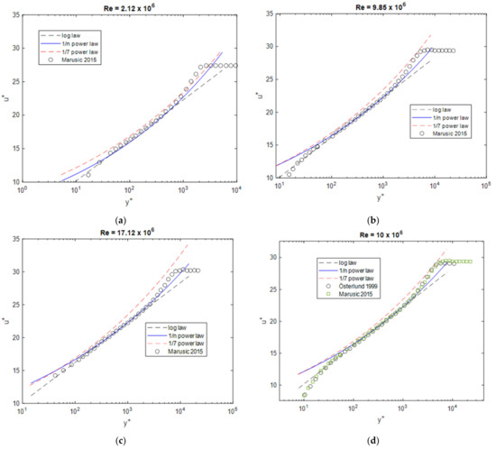
Figure 7.
Boundary layer profiles at different Reynolds numbers compared to the data from Marusic et al. [13] and Österlund [10], (a) Re = 2.12 × 10⁶, (b) Re = 9.85 × 10⁶, (c) Re = 17.12 × 10⁶, (d) Re = 10 × 106.
Figure 8 compares the results with the data from Vallikivi et al. [11]. Again, at high Reynolds numbers, the best agreement is shown for the 1/n power-law. The comparison of the different experimental data (Figure 8e,f) shows differences demonstrating the difficulty of comparability with the experimental data.
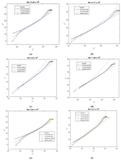
Figure 8.
Boundary layer profiles at different Reynolds numbers compared to the data from Vallikivi et al. [11], Marusic et al. [13], and Österlund [10], (a) Re = 0.05 × 10⁸, (b) Re = 0.17 × 10⁸, (c) Re = 0.6 × 10⁸, (d) Re = 1.65 × 10⁸, (e) 4.91 × 10⁶, (f) 0.17 × 10⁸.
Figure 9 compares the data with the profiles determined by Oweis et al. [14]. Here, a shift can be seen for all experimental profiles compared to the power-law and log law profiles, which increases slightly with decreasing Reynolds number. This is assumed to result from the pressure gradient along the measuring section [21]. Therefore, a corresponding correction with a constant shift of was inserted, with which the 1/n power-law results agree quite well.
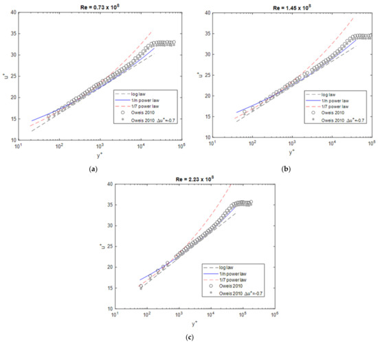
Figure 9.
Boundary layer profiles at different Reynolds numbers compared to the data from Oweis et al. [14], (a) Re = 0.73 × 10⁸, (b) Re = 1.45 × 10⁸, (c) Re = 2.23 × 10⁸.
4. Conclusions
In this paper, a formula for the analytical determination of boundary layer quantities was derived, based on the data from Barenblatt et al. [9] and Buschmann and Gad-el-Hak [6]. Like the 1/7 power-law, the formula is based on a power-law approach for the boundary layer profile, whereby the exponent and intercept are dependent on the Reynolds number.
Subsequently, the results obtained with the formula were compared with current data in the literature. Good agreement was found over a wide range of Reynolds numbers, both for the friction coefficients and the boundary layer thicknesses and profiles themselves.
At the same time, the comparison once again shows the problem of how to normalise experimental data to obtain satisfactory agreement. The classical approach to plot the data over or without considering further boundary conditions shows large deviations in the experimental results. Nevertheless, the general trend confirms the validity of the presented approach. All boundary layer quantities considered can be represented with the same or better approximation to the experimental data than with comparable approaches, especially at high Reynolds numbers. This confirms that the relations for and derived from smaller Reynolds numbers are apparently also valid for higher Reynolds numbers. The quality of the results could be further improved by a comprehensive investigation of correct and values. The same approach can be taken for pipe flows with respective n and k (see [22]).
Funding
This research received no external funding.
Acknowledgments
The author would like to thank Christian Navid Nayeri for the helpful discussions and support.
Conflicts of Interest
The author declares no conflict of interest.
References
- Tschepe, J.; Maaß, J.-T.; Nayeri, C.N.; Paschereit, C.O. Experimental investigation of the aerodynamic drag of roof-mounted insulators for trains. J. Rail Rapid Transit 2019, 234, 834–846. [Google Scholar] [CrossRef]
- Bell, J.; Burton, D.; Thompson, M.; Herbst, A.; Sheridan, J. A wind-tunnel methodology for assessing the slipstream of high-speed trains. J. Wind. Eng. Ind. Aerodyn. 2017, 166, 1–19. [Google Scholar] [CrossRef]
- de Chant, L.J. The venerable 1/7th power law turbulent velocity profile: A classical nonlinear boundary value problem solution and its relationship to stochastic processes. Appl. Math. Comput. 2005, 161, 463–474. [Google Scholar] [CrossRef]
- Tschepe, J.; Nayeri, C.; Paschereit, C. On the influence of Reynolds number and ground conditions on the scaling of the aerodynamic drag of trains. J. Wind. Eng. Ind. Aerodyn. 2021, 213, 104594. [Google Scholar] [CrossRef]
- Barenblatt, G. Scaling laws for fully developed turbulent shear flows. Part 1. Basic hypotheses and analysis. J. Fluid Mech. 1993, 248, 513–520. [Google Scholar] [CrossRef]
- Buschmann, M.H.; Gad-El-Hak, M. Debate Concerning the Mean-Velocity Profile of a Turbulent Boundary Layer. AIAA J. 2003, 41, 565–572. [Google Scholar] [CrossRef]
- George, W.K. Recent Advancements Toward the Understanding of Turbulent Boundary Layers. AIAA J. 2006, 44, 2435–2449. [Google Scholar] [CrossRef]
- Buschmann, M.H.; Gad-el-Hak, M. Turbulent boundary layers: Reality and myth. Int. J. Comput. Sci. Math. 2007, 1, 159–176. [Google Scholar] [CrossRef]
- Barenblatt, G.I.; Chorin, A.J.; Prostokishin, V.M. Analysis of Experimental Investigations of Self-Similar Intermediate Structures in Zero-Pressure Boundary Layers at Large Reynolds Numbers. arXiv 2000, arXiv:math-ph/0002004. [Google Scholar]
- Österlund, J. Experimental Studies of Zero Pressure-Gradient Turbulent Boundary-Layer Flow; KTH: Stockholm, Sweden, 1999; Available online: https://www.mech.kth.se/~jens/zpg/art/zpg_screen.pdf (accessed on 5 January 2022).
- Vallikivi, M.; Hultmark, M.; Smits, A. Turbulent boundary layer statistics at very high Reynolds number. J. Fluid Mech. 2015, 779, 371–389. [Google Scholar] [CrossRef]
- Gorbushin, A.; Osipova, S.; Zametaev, V. Mean Parameters of an Incompressible Turbulent Boundary Layer on the Wind Tunnel Wall at Very High Reynolds Numbers. Flow Turbul. Combust 2021, 107, 31–50. [Google Scholar] [CrossRef]
- Marusic, I.; Chauhan, K.; Kulandaivelu, V.; Hutchins, N. Evolution of zero-pressure-gradient boundary layers from different tripping conditions. J. Fluid Mech. 2015, 783, 379–411. [Google Scholar] [CrossRef]
- Oweis, G.; Winkel, E.; Cutbrith, J.; Ceccio, S.; Perlin, M.; Dowling, D. The mean velocity profile of a smooth-flat-plate turbulent boundary layer at high Reynolds number. J. Fluid Mech. 2010, 665, 357–381. [Google Scholar] [CrossRef]
- de Graaff, D.; Eaton, J. Reynolds-number scaling of the flat-plate turbulent boundary layer. J. Fluid Mech. 2000, 422, 319–346. [Google Scholar] [CrossRef]
- Petrie, H.L.; Fontaine, A.A.; Sommer, S.T.; Brungart, T.A. Large Flat Plate Turbulent Boundary Layer Evaluation; Penn State Applied Research Laboratory Technical Memo File No. 89-207; Penn State Applied Research Laboratory: Reston, VA, USA, 1990; Available online: https://apps.dtic.mil/sti/pdfs/ADA225316.pdf (accessed on 5 January 2022).
- Schlichting, H.; Gersten, K. Boundary-Layer Theory; Springer: Berlin/Heidelberg, Germany, 2017. [Google Scholar] [CrossRef]
- Hoerner, S. Fluid-Dynamic Drag; Hoerner Fluid Dynamics: Bakersfiled, CA, USA, 1965; Available online: http://ftp.demec.ufpr.br/disciplinas/TM240/Marchi/Bibliografia/Hoerner.pdf (accessed on 3 October 2021).
- Schultz-Grunow, F. New Fricitional Resistance Law for Smoothe Plates; NASA Tech Memo No. 986; NASA: Washington, DC, USA, 1941. Available online: https://ntrs.nasa.gov/citations/19930094430 (accessed on 5 January 2022).
- ITTC. Skin Friction and Turbulence Stimulation; Committee Report; ITTC: Ledegem, Belgium, 1957; Available online: https://ittc.info/media/3139/skin-friction-and-turbulence-stimulation.pdf (accessed on 5 January 2022).
- Rona, A.; Monti, M.; Airiau, C. On the generation of the mean velocity profile for turbulent boundary layers with pressure gradient under equilibrium conditions. Aeronaut. J. 2012, 116, 569–598. [Google Scholar] [CrossRef][Green Version]
- Afzal, N.; Seena, A.; Bushra, A. Power Law Velocity Profile in Fully Developed Turbulent Pipe and Channel Flows. J. Hydraul. Eng. 2007, 133, 1080–1086. [Google Scholar] [CrossRef]


Publisher’s Note: MDPI stays neutral with regard to jurisdictional claims in published maps and institutional affiliations. |
© 2022 by the author. Licensee MDPI, Basel, Switzerland. This article is an open access article distributed under the terms and conditions of the Creative Commons Attribution (CC BY) license (https://creativecommons.org/licenses/by/4.0/).