The Capillary Waves’ Contribution to Wind-Wave Generation

Abstract

Published theories and observations have shown that dissipation of gravity waves implies frequency downshifting of wave energy. Hence, for wind-waves, the wind energy input to the highest frequencies is of special interest. Here it is shown that this input is vital, because the direct wind energy input obtained by the air-pressure’s work on most gravity waves is slightly less than what the waves need to grow. Further, the wind’s input of the angular momentum that waves need to grow is found to be absent at most gravity wave frequencies. The capillary waves that appear at the surface of the sea when the wind is blowing solve these problems. To demonstrate this, an extension of linear wave theory is established to study possibilities and limitations for transfer of energy and angular momentum from the wind to waves through these frequencies. The theory describes regular, gravity–capillary waves with constant amplitude under laminar conditions. It includes surface tensions, viscosity, gravity and a wind-generated shear current, and shows that these waves—contrary to most gravity waves—receive more energy from the wind than they dissipate and angular momentum they cannot keep. Hence, the problem of the missing input of energy and angular momentum from wind to gravity waves is solved by transfers through the capillary waves. This implies that capillary waves are vital to obtain growing gravity waves.

1. Introduction

When wind-waves grow, capillary waves are usually present on major parts of the surface of the sea. Under stable wind conditions, a continuous wave spectrum exists between the low-frequency peak and the capillary waves at the high-frequency tail, called the saturation range. According to [1], frequency downshifting of gravity waves is a consequence of dissipation, particularly due to breaking waves. It implies that some wind energy must enter the waves at the high-frequency tail. As shown in [2] and elaborated in [3], progressive waves also need angular momentum to exist. In [2,4] it is shown that if the wave’s angular momentum is conserved, dissipation implies frequency downshifting of gravity waves. An aim here is therefore to learn to what extent the capillary waves supply energy and angular momentum to gravity waves.

According to [5], there is an “absence of fundamental understanding” of wind-wave generation. It is stated more specifically in [6]: “In particular, the role of molecular viscosity, generation of capillary ripples, and microbreaking or breaking has not been clearly identified and quantified up to now”. The aim here is to approach an answer to such problems.

Molecular shear stresses due to capillary waves and wind-induced shear flows are strongest in the upper millimetres of the sea—in the thin, vortical wind-drift layer—where capillary waves dominate the dynamics. A linear theory for regular high-frequency waves in a viscous shear flow is therefore established in Section 2. It is the basis for the study of these wave’s contribution to the wind-wave generation process in the following sections.

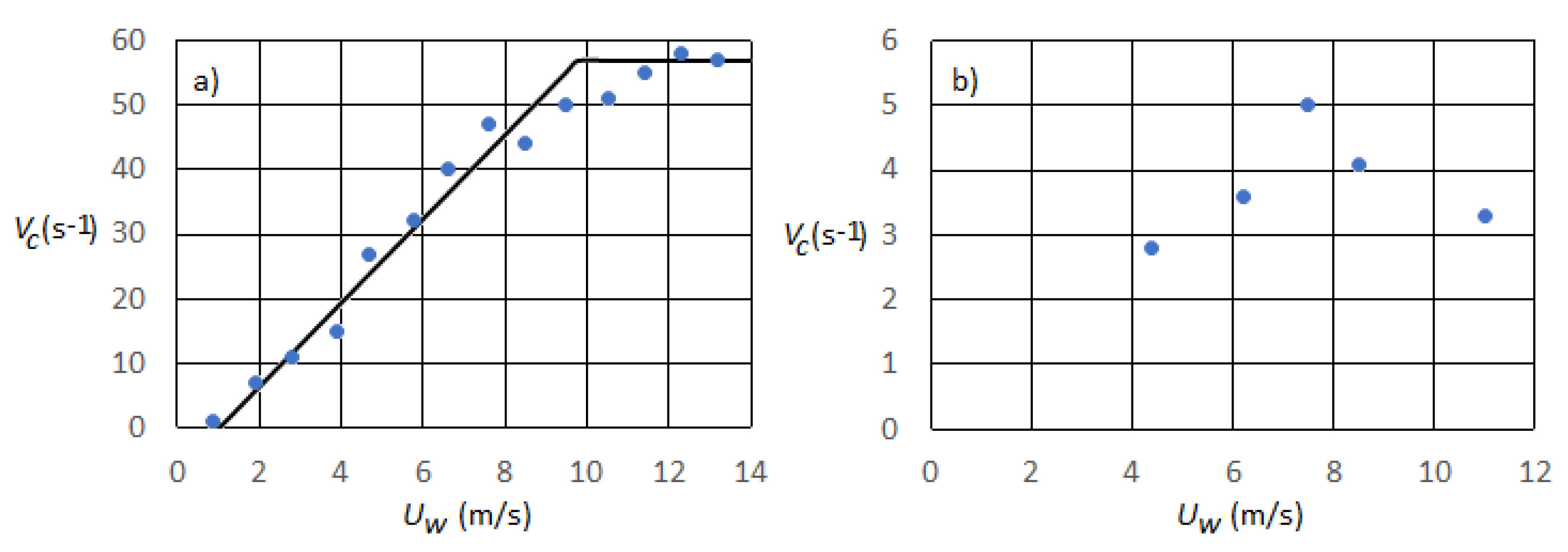
Published measurements of wind-driven currents [7,8,9] show, within the accuracy of the measurements, a current with constant vorticity immediately below the surface. Vorticities of currents are available from two of them. They differ considerably. One dataset is published in Figure 5a in [9]. The author states that “The current immediately below the surface varies linearly with depth”. The data shown in Figure 1a are extracted from Figure 5a in [9]. They show the current $U_C\left(z\right)$ as a linear function of the vertical coordinate $z$ in the upper 3 mm of the water for a series of different wind speeds $U_w$. Within the accuracy of the measurements, the vorticity of the current, $V_C\equiv d{U}_C/dz$, was found to be a function of $U_w$ but independent of the distance from the surface and the time t. Figure 1a is based on these results, where the broken line is:

$$V_C=\left\{\begin{array}{cc}6.5 {\mathrm{m}}^{-1} \left(U_w-1 \mathrm{m}/\mathrm{s}\right)& (1 \mathrm{m}/\mathrm{s}\le U_w<9.77 \mathrm{m}/\mathrm{s})\\ 57{ \mathrm{s}}^{-1}& \left(9.77 \mathrm{m}/\mathrm{s}\le U_w\le 14 \mathrm{m}/\mathrm{s}\right).\end{array}\right.$$

(1)

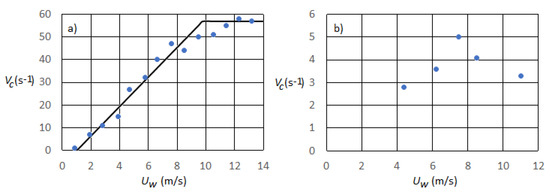
Figure 1. The current’s vorticity $V_C$ as a function of the wind speed $U_w$ in the upper 3 mm below the surface. (a) Data from [9], Figure 5a. Each point is based on two to four data points. (b) Data from [10], Figure 2. Each point is based on two data points.

Be aware that $V_C$ is most likely not zero for wind speeds below 1 m/s.

Similar data are available from Figure 2 in [10], here shown in Figure 1b. Their mean value of $V_C$ is 3.8 s⁻¹. Even if their vorticities are based on data from only two depths, and the surface values therefore may deviate from the values in Figure 1b, the shown vorticities in the upper 3 mm are an order of magnitude smaller than the values in [9].

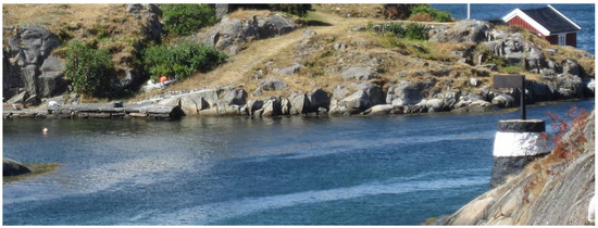
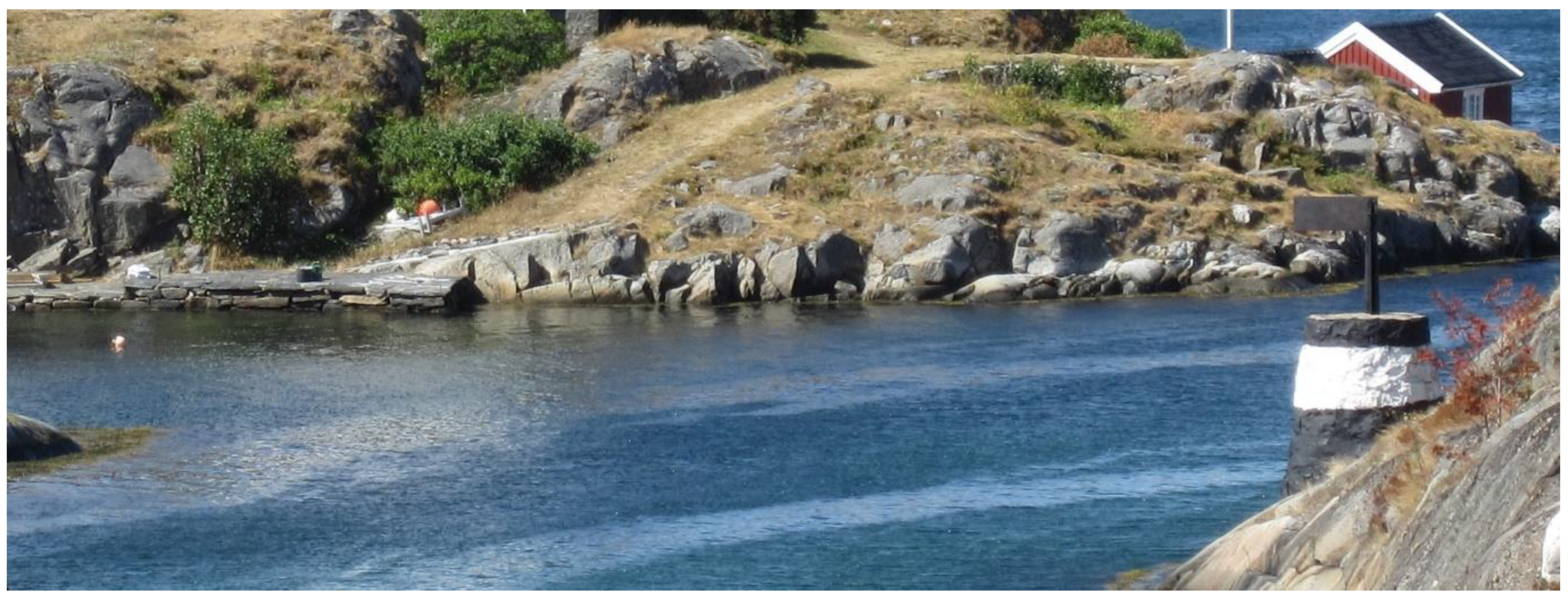
Figure 2. Wind-wave generation in Gamle Hellesund. Capillaries cover the dark areas. The light ribbons without capillaries are common there during rising tides, when the current flows towards the right. The wind blew towards the camera. Estimated wind speed: 5 m/s. Water temp.: 19 °C. Current: 5–10 cm/s.

In [8] it is shown that the presence of turbulence in the upper millimetres implies a much smaller vorticity compared to laminar conditions at the same wind speed. Evidence of the two regimes is visible when the wind blows (see Figure 2). Blank ribbons show where capillary waves are absent. A life at the seaside has taught me that similar blank areas are observed at many almost fixed locations without plants that reach the surface. They are therefore not the result of debris or pollutions drifting by. There is no significant fresh water source nearer the open sea in the area. Hence, during the dry summers in the area, a freshwater layer during rising tides is unlikely. Similar blank ribbons are common in the turbulent wakes behind boats and ships. In the absence of other alternatives, the conclusion is therefore that the upper millimetres of the sea in the area consist of homogenous water that usually is partly turbulent and partly laminar. Further, the vorticity of the current is supposed to be sufficiently constant so as to be treated as though it is not a function of the time and the distance below the surface. As nothing but surface values are needed until Section 3.5, a further discussion of the problem is omitted until then.

On calm, rainy days, a similar difference between blank and rough surfaces can be observed. Then the surface is separated in areas where some appear blank with small rings from the raindrops while the rest appear as continuous rough surfaces—the result of a myriad of intersecting rings with an average diameter much bigger than the average diameter of the rings at the blank parts of the surface. Turbulence and absence of turbulence may explain the difference in this case, as well. Why it is like that is not further discussed.

An overwhelming number of papers explore the existence of surface waves and currents. Of these, only the few papers that contain relevant information for the present theory are referred to. On the other hand, particularly due to the consequences of including angular momentum, the present theory may be useful in future works on waves.

2. Basic Theory of Wind-Supported Waves

2.1. Introduction

This theory describes waves with a constant amplitude under laminar conditions, here denoted wind-supported waves. It adopts (1) (based on [9]) to obtain a connection between waves and wind, even if the measurement technique in [9] implies that the accuracy should be questioned.

As in [11,12], waves in a shear flow are studied. However, while gravity waves in a viscous fluid are studied in [12], surface tension is also included here. Since the water depth is of minor importance, deep-water waves are considered. The theory is based on the theory of “free waves”, e.g., Airy’s linear, two-dimensional, regular wave theory [13] or similar. The term “capillaries” refers to waves at frequencies where surface tension is dominating over gravity, while the term “gravity waves” refers to waves at lower frequencies where gravity dominates the dynamics.

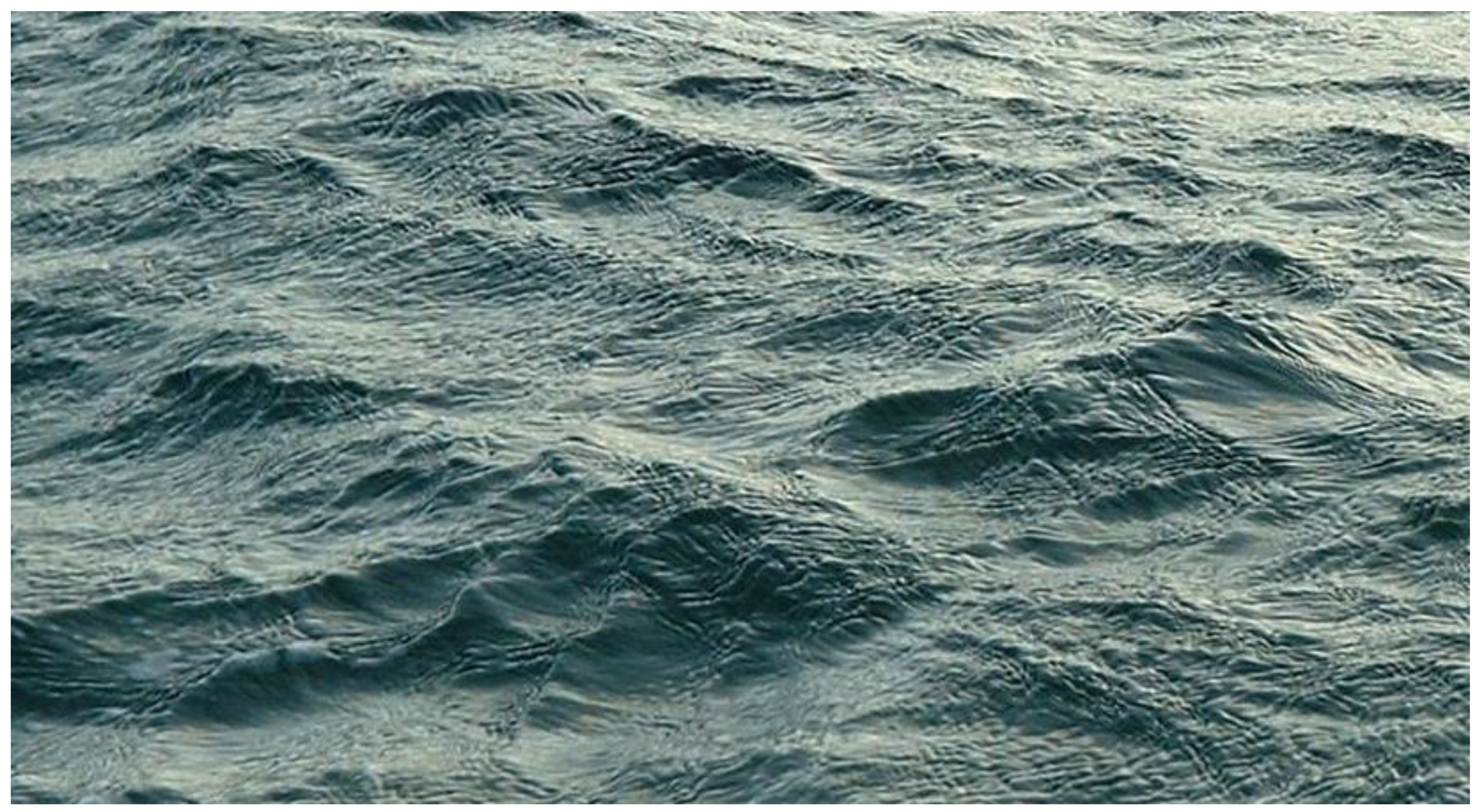
The aim is to study the capillaries’ part in the wind-wave generation process by elementary analytical tools. Such waves cover major parts of the surface in the upper left part of Figure 3. In its lower part, you can see many cases of capillaries at sharp peaks with smooth troughs at the other side of the peak. They seem to be similar to the parasitic capillaries studied among others in [14,15].

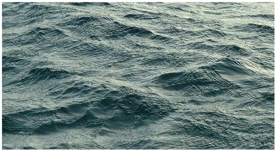
Figure 3. Waves generated by a fresh breeze from the right. Fetch length ≈ 250 m.

As a basis for the theory, clean, homogenous water is considered. Hence, contaminations that imply a variable surface tension along the surface, as studied in [16], or oil on the surface, as discussed in [17], are not covered by the theory.

Since Figure 3 shows that long-crested, wind-supported capillaries appear when gravity waves are present, a two-dimensional wave theory is supposed to be relevant for the study of such waves. The waves are described by adding terms that support vertical flows of energy and momentum to the free wave theory.

2.2. Basis

The theory adopts Eulerian description in a coordinate system where the water far below the surface is at rest. The unit vectors $\mathit{i}, \mathit{j}$ and $\mathit{k}$ are in the directions of the x, y and z axes, respectively. The current $\tilde{U}\left(x,z,t\right)$ is a function of the time t when measured in a fixed point, since the current follows the sinusoidal surface up and down. Its mean value over a wave period is $U\left(z,t\right).$

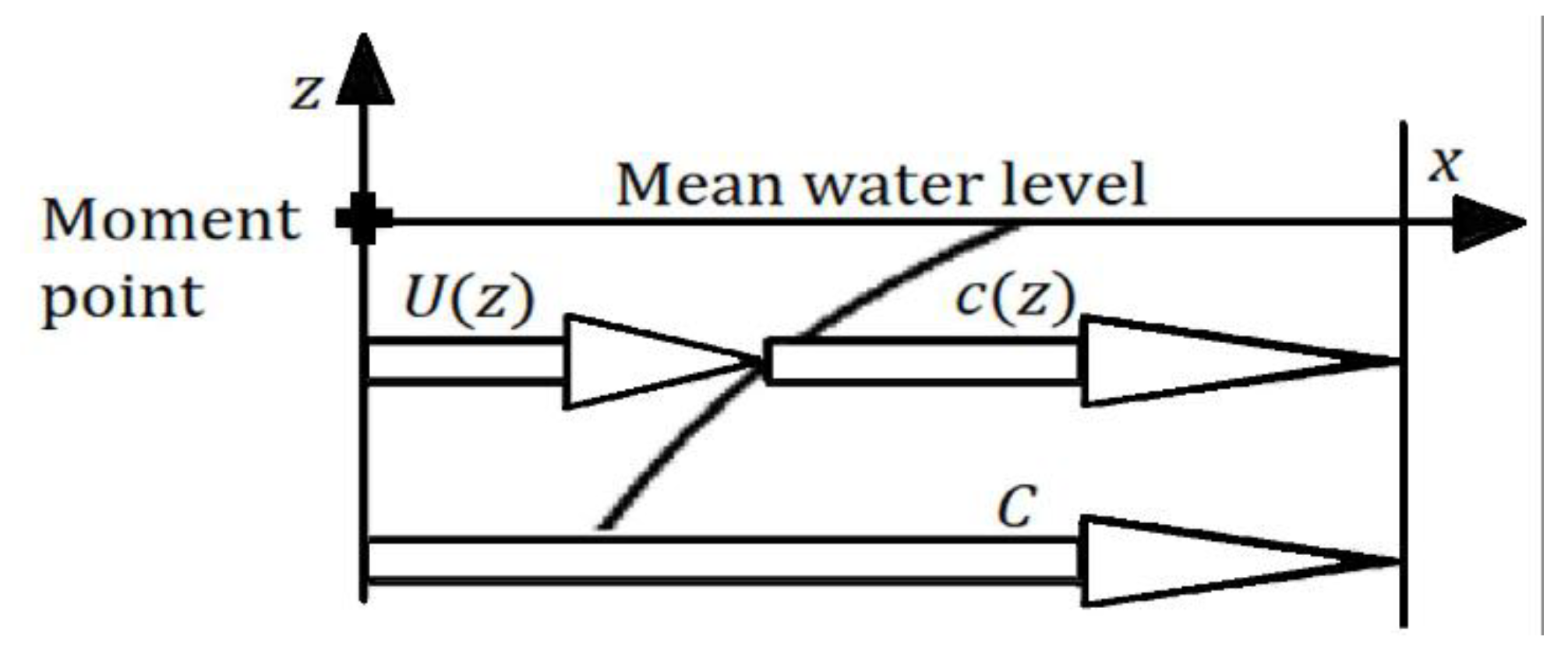
As shown in Figure 4, two different phase speeds are adopted: $C$ relative to the origin and $c\left(z\right)$ relative to $U.$ Similarly, the circular wave frequency relative to the origin is $\mathsf{\Omega }$ while the circular frequency of the water is $\omega \left(z\right)$. From now on, arguments are usually included the first time a variable appears only.

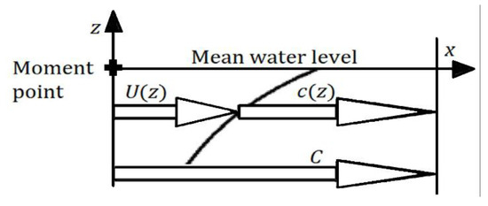
Figure 4. C is the phase speed relative to the origin and $c\left(z\right)$ the phase speed relative to the current $U\left(z\right)$. The y axis points away from the reader.

The shear stresses from the wind imply that $U$ is a function of $t$ so that $C$ and $\mathsf{\Omega }$ are functions of $t$, as well. However, the acceleration of $U$ is negligible compared to the harmonic acceleration terms. Hence, $C$ and $\mathsf{\Omega }$ are treated as constants and $U$ as a function of $z$ only. Further, the wave number is $\kappa =2\pi /\lambda$ where $\lambda$ is the wavelength.

As shown in Figure 4, if the velocities are connected by

$$C=U+c\left(z\right)$$

(2)

then $\kappa =\mathsf{\Omega }/C=\omega \left(z\right)/c\left(z\right)$. Hence, when (2) is multiplied by $\kappa$, then

$$\mathsf{\Omega }=\kappa U+\omega .$$

(3)

The vertical position of a fluid element is

$$\tilde{\eta }\left(x,z,t\right)=\eta \left(z\right)\cos \left(\theta \left(x,z,t\right)\right)={\eta }_0{\mathrm{e}}^{kz}\cos \theta .$$

(4)

The $\widetilde{ }$ shows that a variable, in this case $\tilde{\eta }$, has at least one sinusoidal term—here, with amplitude $\eta$. Index 0 shows that a variable, in this case ${\eta }_0$, is the value of $\eta$ at $z=0$.

The constant $k$ in the exponent of the exponential function does not have to be equal to $\kappa$. Hence, we allow two wave numbers. Further, $\theta$ is allowed to be a function of $z$:

$$\theta =\mathsf{\Omega }t-\kappa x-\beta \left(z\right)$$

(5)

where $\beta$ is a phase angle relative to $z=0$. Hence, $\beta \left(0\right)\equiv {\beta }_0=0$.

The velocity is described by its two components $\tilde{u}\left(x,z,t\right)$i and $\tilde{w}\left(x,z,t\right)\mathit{k}$. When higher order, harmonic terms are omitted, then $\tilde{w}\equiv d\tilde{\eta }/dt=\partial \tilde{\eta }/\partial t+U\partial \tilde{\eta }/\partial x$, from which $\tilde{w}=-\eta \left(\mathsf{\Omega }-\kappa U\right)\sin \theta$. By adopting (3),

$$\tilde{w}=-\omega \eta \sin \theta .$$

(6)

The amplitude of $\tilde{w}$ is then

$$w=\omega \eta .$$

(7)

The wave’s contribution to the horizontal velocity component $\tilde{u}$ is

$${\tilde{u}}_W\left(x,z,t\right)=u\left(z\right)\left[\cos \theta +\alpha \left(z\right)\sin \theta \right].$$

(8)

Here, $\alpha$ allows a phase difference between ${\tilde{u}}_W$ and $\tilde{\eta }$. It implies that the dynamical pressure of the water at the surface, and therefore of the air at the surface, can be partly in phase with the vertical velocity of the water. In that way, it allows for the sheltering effect Refs. [18,19].

Let $\prime$ replace $\partial /\partial z$ and let $V\equiv U^{\prime }$. Then, the mean value of the horizontal component of the equation of motion is

$$\frac{\partial U}{\partial t}=\nu V^{\prime }$$

(9)

where $\nu$ is the kinematic viscosity. Near the surface, the acceleration of $U$ is negligible compared to the accelerations of $\tilde{u}$ and $\tilde{w}$. It is therefore sufficiently accurate to consider that $\partial U/\partial t=0$. Then, (9) implies that $V^{\prime }=0$, i.e., as expected from the measurements in [9]. It is not so throughout the wave zone at depths where the acceleration of $\tilde{u}$ and $\tilde{w}$ are of the same order of magnitude as $\partial U/\partial t$. There, $V^{\prime }$ might be positive, e.g., a logarithmic function. In Figure 3, however, where the capillaries are riding on long gravity waves compared to the wave lengths of the capillaries, it is hardly relevant to expect any such current, as the vorticity of the flow near the surface of gravity waves varies between negative and positive values. Hence, the wind drift implies variations in $V$ along the surface, and under such conditions, $V^{\prime }$ may be nonzero, even at the surface.

It should also be noted that the increase in momentum due to wind shear stresses does not end up as increasing currents only, but also as Stokes drift of the growing gravity waves. It is a possible explanation for why $U$ was not observed as a function of $t$ in [9], and therefore why $V^{\prime }=0$. The shear force obtained by $\rho \nu V$ provides a vertical flux of momentum downwards. The opposite flux may be provided by the term $\rho \tilde{u}\tilde{w}$. Then the curvature of $V$ is reduced. Thus, to keep the theory simple, we let $V^{\prime }=0$ and leave the problems of a variable $V$ to be solved by other means.

Since the current in a fixed point is a function of an oscillating vertical distance from the surface, and $V$ is supposed to not be a function of $z$, the horizontal component of the current in a fixed point is defined as $\tilde{U}=U-V\tilde{\eta }$, so that

$$\tilde{U}=U-V\eta \cos \theta .$$

(10)

When (8) and (10) are inserted in the sum of the contributions from current and waves, i.e., $\tilde{u}=\tilde{U}+{\tilde{u}}_W$, then

$$\tilde{u}=U+\left(u-V\eta \right)\cos \theta +\alpha u\sin \theta .$$

(11)

Since $V$ is not a function of $z$, $c=c_0-Vz$, so that

$$\omega ={\omega }_0-\kappa Vz.$$

(12)

In the following, relations between the variables are established. Since $U$ and $V$ may not be exactly constant, approximations are frequently adopted to simplify formulae when it can be done without significant losses of accuracy.

2.3. Continuity

The equation of continuity is $\partial \tilde{u}/\partial x+\tilde{w}\prime =0$. By differentiation of (11), it follows that $\partial \tilde{u}/\partial x=\kappa \left(u-V\eta \right)\sin \theta -\alpha \kappa u\cos \theta$ and by differentiation of (6), it follows that ${\tilde{w}}^{\prime }=\left(\kappa V\eta -\omega {\eta }^{\prime }\right)\sin \theta +{\beta }^{\prime }w\cos \theta$. Hence, the equation of continuity can be written

$$\left({\beta }^{\prime }w-\alpha \kappa u\right)\cos \theta +\left(\kappa u-\omega {\eta }^{\prime }\right)\sin \theta =0.$$

(13)

As (13) is valid for any θ, two separate equations are obtained:

$$\frac{u}{w}=\frac{{\beta }^{\prime }}{\alpha \kappa }$$

(14)

and

$$u=c{\eta }^{\prime }.$$

(15)

It is practical to define a constant $I=u/w$. ($I=1$ for deep water free waves.) Then, from (7)

$$u=I\omega \eta .$$

(16)

Equations (15) and (16) imply that $I\omega \eta =c{\eta }^{\prime }$. Since $c=\omega /\kappa$, it follows that ${\eta }^{\prime }=I\kappa \eta$, where $I\kappa$ is a product of two constants. By choosing $k=I\kappa$, then, as in (4),

$$\eta ={\eta }_0{\mathrm{e}}^{kz}.$$

(17)

Let

$$B=I-\frac{V}{\omega }$$

(18)

and to avoid the product $I\alpha$ appearing frequently, let

$$\epsilon =I\alpha .$$

(19)

Then, (11) can be written

$$\tilde{u}=U+\omega \eta \left(B\cos \theta +\epsilon \sin \theta \right).$$

(20)

In summary, the relative wave number is

$$I=\frac{k}{\kappa }=\frac{u}{w}=\frac{{\beta }^{\prime }}{\alpha \kappa }=\frac{\epsilon }{\alpha }=B+\frac{V}{\omega }.$$

(21)

It shows how continuity restricts the dynamics of waves in an incompressible fluid with shear currents.

2.4. The Air Pressure at the Surface

If regular waves are described in a coordinate system where $C=0$, then, since the amplitude is constant, what we get is a flow of water below a surface at rest. Since the air pressure at the surface, ${\tilde{p}}_{air}$, acts perpendicularly to the velocity of every fluid element at the surface, it cannot transfer energy through the surface at any point, not even to steep waves. Hence, when no other waves are present, viscous shear stresses replace dissipated wave energy and increase the thermal energy of the water (the temperature) while the air pressure’s work is zero.

In general, work is not invariant to coordinate transformations. This case, however, is different. Since the wave height is constant, the mechanical energy of the system of waves and currents is not a function of $t$, whether $C=0$ or $C\ne 0$. In addition, the temperature, i.e., the thermal energy, is the same in both cases. Since the work performed by shear stresses is a function of the local vorticity and not $C$, it is the same in both cases. Therefore, to avoid violation of the energy principle, the total work performed by the air pressure when $C\ne 0$ equals the work when $C=0$. As it is zero when $C=0$, it is also zero when $C\ne 0$. It implies that ${\tilde{p}}_{air}$ is constant in time and space when the wave height is constant.

The air pressure is not constant for growing waves, however. That problem is treated mathematically in Section 3.1. Neither is it necessarily constant if the waves ride on waves with another phase velocity, as in Figure 3, since it is then impossible to find a coordinate system where the surface is at rest. However, the deviations from a constant pressure over a wavelength are supposed to be negligible for capillaries with wavelengths decades smaller than the wavelengths of the gravity waves they are riding.

2.5. The Equation of Motion, Horizontal Component

The derivatives needed in the following are shown in Table 1, together with the equation numbers from which they are derived. In (T11) and (T22)

$${\tilde{a}}_x=\frac{\mathrm{d}\tilde{u}}{\mathrm{d}t}=\frac{\partial \tilde{u}}{\partial t}+U\frac{\partial \tilde{u}}{\partial x}+V\tilde{w}$$

(22)

and

$${\tilde{a}}_z=\frac{\mathrm{d}\tilde{w}}{\mathrm{d}t}=\frac{\partial \tilde{w}}{\partial t}+U\frac{\partial \tilde{w}}{\partial x}.$$

(23)

Table 1. Derivatives. Approximations: $\partial U/\partial t=0, V^{\prime }=0, {\epsilon }^2=0$.

Formula	Derived from; by Using	Equation
${\eta }^{\prime }=k\eta$	(17)	(T1)
$\partial \theta /\partial x=-\kappa$	(5)	(T2)
$\partial \theta /\partial t=\mathsf{\Omega }$	(5)	(T3)
${\theta }^{\prime }=-\epsilon \kappa$	(5); (14), (19)	(T4)
${\omega }^{\prime }=-\kappa V$	(3)	(T5)
$B^{\prime }=-\kappa {\left(I-B\right)}^2$	(18); (T5)	(T6)
$N^{\prime }=\kappa N\left(I-B\right)$	(27); (18), (T5)	(T7)
${\left(B\omega \right)}^{\prime }=-kV$	(18), (21); (T5)	(T8)
$\partial \tilde{u}/\partial t=-\omega \mathsf{\Omega }\eta (B\sin \theta -\epsilon \cos \theta )$	(20); (T3)	(T9)
$\partial \tilde{u}/\partial x=\omega \kappa \eta (B\sin \theta -\epsilon \cos \theta )$	(20); (T2)	(T10)
${\tilde{a}}_x=-{\omega }^2\eta \left(I\sin \theta -\epsilon \cos \theta \right)$	(22); (6), (T9), (T10)	(T11)
${\partial }^2\tilde{u}/\partial x^2=-\omega {\kappa }^2\eta (B\cos \theta +\epsilon \sin \theta )$	(T10); (T2)	(T12)
${\tilde{u}}^{\prime }=V+\eta \left\{k\left(B\omega -V\right)\cos \theta +\omega \left(2 \epsilon \kappa B+{\epsilon }^{\prime }\right)\sin \theta \right\}$	(20); (18), (T1), (T4), (T5), (T6)	(T13)
${\tilde{u}}^{″}=\eta \{k^2\left(B\omega -3V\right)\cos \theta +\left[3\omega \left(\epsilon k^2+{\epsilon }^{\prime }\kappa B\right)\left.-6\epsilon \kappa kV\right]\left.\sin \theta \right\}\right.$	(T15); (18), (T1), (T4), (T5), (T8), (T10)	(T14)
${\nabla }^2\tilde{u}=\eta \left\{\left[B\omega {\kappa }^2\left(I^2-1\right)\right.\right.-3\epsilon \omega \kappa \left({\epsilon }^{\prime }+\epsilon \kappa B\right)\left.-3k^{2}V\right]\cos \theta +\left[\omega \left(3\epsilon k^2-\epsilon {\kappa }^2+3{\epsilon }^{\prime }\kappa B\right)\right.\left.-6\epsilon \kappa kV\right] \left.\sin \theta \right\}$	(T12), (T14)	(T15)
$\partial \tilde{w}/\partial t=-\mathsf{\Omega }\omega \eta \cos \theta$	(6); (T3)	(T16)
$\partial \tilde{w}/\partial x=\omega \kappa \eta \cos \theta$	(6); (T2)	(T17)
${\partial }^2\tilde{w}/\partial x^2=\omega {\kappa }^2\eta \sin \theta$	(T17); (T2)	(T18)
${\tilde{w}}^{\prime }=-\kappa \omega \eta \left(B\sin \theta -\epsilon \cos \theta \right)$	(6); (18), (T1), (T4), (T5)	(T19)
${\tilde{w}}^{″}=-\kappa \eta \left[\left(Ik\omega -2kV\right)\sin \theta \right.\left.-\omega \left(2\epsilon \kappa B+{\epsilon }^{\prime }\right)\cos \theta \right]$	(T19); (18), (T1), (T4), (T5), (T8)	(T20)
${\nabla }^2\tilde{w}=-\kappa \eta \left\{\left[\kappa \omega \left(I^2-1\right)-2kV\right]\sin \theta \right.\left.-\omega \left[2\epsilon \kappa B+{\epsilon }^{\prime }\right]\cos \theta \right\}$	(T18), (T20)	(T21)
${\tilde{a}}_z=-{\omega }^2\eta \cos \theta$	(23); (6), (T16), (T18)	(T22)
$\partial \tilde{p}/\partial x=\rho \omega u\sin \theta$	(28); (T2)	(T23)
${\tilde{p}}^{\prime }=\rho I\omega \eta \left[\left(I\omega -2V\right)\cos \theta +\epsilon \omega \sin \theta \right]$	(28); (16), (T1), (T4), (T5)	(T24)

In (22) and (23), second order terms of the harmonic functions are omitted.

When (9) is taken into account, the horizontal component of the equation of motion is

$$\frac{\partial }{\partial x}\tilde{p}\left(x,z,t\right)=-\rho {\tilde{a}}_x+\rho \nu {\nabla }^2\tilde{u}$$

(24)

where $\tilde{p}$ is the pressure, $\rho$ the density and ${\nabla }^2={\partial }^2/\partial x^2+{\partial }^2/\partial z^2$. When (T 11) and (T15) are adopted,

$$\begin{gathered} \frac{\partial \tilde{p}}{\partial x}=\rho \eta \left\{\left[-\epsilon {\omega }^2+\nu {\kappa }^2\left(I^2-1\right)B\omega \right.\right.\left.-3\nu k^{2}V\right]\cos \theta \\ +\left[I{\omega }^2+\nu \left(3\epsilon k^2+3{\epsilon }^{\prime }\kappa B-\epsilon {\kappa }^2\right)\omega \right.\left.-6\epsilon \nu \kappa kV\right]\left.\sin \theta \right\}. \end{gathered}$$

(25)

From Section 2.4 it follows that the air pressure at the surface, ${\tilde{p}}_{air}$, is not a function of $x$. Then, the water pressure is proportional $\cos \theta$ so that $\partial \tilde{p}/\partial x\propto \sin \theta$. Hence, the sum of the terms in the brackets of the $\cos \theta$ term is zero. It implies that

$$\epsilon =\left[\left(3B-2I\right)I^2-B\right]N$$

(26)

where

$$N=\frac{\nu {\kappa }^2}{\omega }.$$

(27)

Since $\left|\epsilon \right|<5·{10}^{-4}$ for all values of $\lambda$ and $z$, then, within the accuracy of the theory, $\epsilon =\alpha =0$. Then the terms in the brackets of the $\sin \theta$ term of (25) are reduced to $I{\omega }^2$. Hence, integration of (25) with respect to $x$ implies that

$$\tilde{p}={\tilde{p}}_{air}+\rho cu\cos \theta .$$

(28)

2.6. Phase Speed and Frequency

Phase speeds of gravity waves on shear currents of various $z$-dependencies are calculated by [20,21,22,23,24,25] and others. They found that the phase speed relative to the water at the surface is slightly smaller than the speed of free waves and that the effect of wind is small. An alternative approach follows, based on the present wave theory.

According to Equation (3.6:9) in [26], the pressure difference across the surface is

$${\tilde{p}}_{air}-{\tilde{p}}_s=-\tau \frac{{\partial }^2{\tilde{\eta }}_0}{\partial x^2}$$

(29)

where $\tau$ is the surface tension. Since ${\tilde{p}}_{air}$ is constant when the amplitude is constant, the harmonic terms of (29) are

$${\tilde{p}}_s=\tau {\kappa }^2{\eta }_0\cos {\theta }_0.$$

(30)

Equation (28) implies that the pressure at $z=0$ (where ${\tilde{\eta }}_0\ge 0$) is ${\tilde{p}}_0=\rho c_0{u}_0\cos {\theta }_0$ and from (16) it follows that $u_0=I{\omega }_0{\eta }_0$. Hence,

$${\tilde{p}}_0=\rho I{c}_0{\omega }_0{\eta }_0\cos {\theta }_0.$$

(31)

The acceleration of gravity ($g$) implies that $\tilde{p}\left(x,z,t\right)={\tilde{p}}_0-\rho gz$. Hence, at the surface level, where $z={\eta }_0\cos \theta$,

$${\tilde{p}}_s={\tilde{p}}_0-\rho g{\eta }_0\cos {\theta }_0.$$

(32)

By inserting from (30) and (31) in (32), then $\tau {\kappa }^2=\rho c_{0}I{\omega }_0-\rho g$, so that

$$c_0=\frac{{\omega }_0}{\kappa }=\sqrt{\frac{1}{I}\left(\frac{g}{\kappa }+\frac{\kappa \tau }{\rho }\right)}.$$

(33)

According to [27], Section 267, Equation (2), the phase speed of free waves $c_f={\left(g/\kappa +\kappa \tau /\rho \right)}^{1/2}$. Hence, with ${\omega }_f$ as the circular frequency of free waves,

$${\left(\frac{c_0}{c_f}\right)}^2={\left(\frac{{\omega }_0}{{\omega }_f}\right)}^2=\frac{1}{I}.$$

(34)

According to [20,21,22,23,24,25], $c_0$ is slightly smaller than $c_f$. Hence, $I$ must be slightly greater than 1.

2.7. The Equation of Motion, Vertical Component

The harmonic terms of the vertical component of the equation of motion are

$$\rho {\tilde{a}}_z=-{\tilde{p}}^{\prime }+\rho \nu {\nabla }^2\tilde{w}.$$

(35)

By inserting from (T22), (T24) and (T21), and since $\epsilon =0$, the $\cos \theta$ terms imply that

$$-\omega =-\left(I^2\omega -2VI\right)+\nu \kappa \left(2\epsilon \kappa B-\kappa \right).$$

(36)

By adopting (18) and (27), (36) implies that

$$B=\frac{I^2+1-N}{2I}.$$

(37)

For all frequencies, (37) implies that $B_0=1$. ($B_0$ and $N_0$ are the values of $B$ and $N$ at $z=0$). Hence, the difference between $u$ and $w$ vanishes at the surface. By using $B_0=1$ in (37),

$$I=1+\sqrt{N_0}.$$

(38)

2.8. Numerical Results

Numerical values are shown in Table 2. The case where $\lambda =3.08$ mm at 0 °C is omitted, because then the upper line of (1) is not valid. Under breeze conditions, the table shows that wave lengths between 3 and 5 mm are dominating, a result that is easily confirmed by visual observations of the sea.

Table 2. Numerical values under laminar surface conditions.

λ (mm)		3.08	4.00	5.00	7.00	10.00	15.00	30.00	40.00	Input
κ (mm−1)		2.040	1.571	1.257	0.898	0.628	0.419	0.209	0.157	2π/λ
ω0 (s−1) ω0 (s−1)	20 °C	777.20	531.93	386.80	242.75	152.75	95.69	51.55	42.24	(33)
	0 °C		526.11	385.15	240.99	151.16	94.32	50.48	42.07	(33)
N0·103	20 °C	5.35	4.64	4.08	3.32	2.58	1.834	0.851	0.584	(27)
N0·103	0 °C		8.44	7.43	6.03	4.69	3.33	1.539	1.056	(27)
I	20 °C	1.073	1.068	1.064	1.058	1.051	1.043	1.029	1.024	(38)
I	0 °C		1.092	1.086	1.078	1.069	1.058	1.040	1.032	(38)
V (s−1)	20 °C	56.87	36.23	24.71	13.98	7.77	4.08	1.504	1.021	(18)
V (s−1)	0 °C		48.34	32.99	18.68	10.37	5.48	2.01	1.367	(18)
Uw (m/s)	20 °C	≥ 9.75	6.57	4.80	3.15	2.18	1.62	1.23	1.16	(1)
Uw (m/s)	0 °C		8.44	6.08	3.87	2.60	1.84	1.31	1.21	(1)

$\tau =0.074 {\mathrm{N} \mathrm{m}}^{-1}, g=9.81 {\mathrm{m} \mathrm{s}}^{-2}, \rho =1000 {\mathrm{kg} \mathrm{m}}^{-3}, \nu \left(0 °\mathrm{C}\right) =1.8 {\mathrm{mm}}^2{\mathrm{s}}^{-1}, \nu \left(20 °\mathrm{C}\right) =1.0 {\mathrm{mm}}^2{\mathrm{s}}^{-1}$. (The wind speed $U_w$ is not calculated by the theory but based on (1), i.e., measurements).

$I$ can be calculated both from (18) and (38): $I=1+V/{\omega }_0=1+\sqrt{N_0}$ so that

$$V={\omega }_0\sqrt{N_0}\equiv \sqrt{\nu {\kappa }^2{\omega }_0}.$$

(39)

It shows that if $V$ is reduced to the values shown in Figure 1b, the viscosity must be reduced below molecular viscosity if the theory shall provide frequencies like those observed. The observed wind-generated capillaries at sea therefore imply a laminar boundary layer.

The relationship between $\lambda$ and $U_w$ confirms—at least approximately—these visual observations: the shortest wavelengths are observed at the highest wind speeds, and the wavelength is approximately 3 mm at a fresh breeze, while wavelengths above 40 mm can be observed at very light winds. Figure 5 shows capillaries at an intermediate wavelength before wave–wave interactions had time to generate other waves. The wave heights seem to be approximately 1 mm or less for all wavelengths, including the capillaries in Figure 2, Figure 3 and Figure 5.

Figure 5. Wind-supported capillaries and autumn leaves in a pond shortly after a sudden onset of a gentle breeze. Stipulated wavelength: 7–10 mm. Stipulated wave height: 1 mm. Temp.: 0 °C.

The author is not aware of published simultaneous measurements of $\lambda$ and $V$. Since the relation between the two follows from adopting fundamental equations of fluid dynamics, there is in any case no room for alternatives to those given in Table 2.

While the theory gives a reasonable relationship between wind measurements in [9] and the wavelengths of high-frequency waves, it does not at all explain the existence of ocean waves at much lower frequencies. If wind-supported waves could have such frequencies, the measurements in [9] would imply a wind speed below 1 m/s. At such frequencies, the present theory is reduced to an ordinary, linear gravity wave theory where the viscosity is negligible, i.e., to Airy’s wave theory [13].

If the present theory is relevant for the description of the capillaries in Figure 3, the theory must show that the energy input from the wind to the waves is sufficient to overcome the dissipation. If the wind energy input exceeds the dissipation, then wave–wave interactions may transfer the excess energy to lower wave frequencies. To investigate this, the vertical energy flow to the waves and the dissipation inside the waves are calculated in Section 3. Since the theory of free gravity waves is a special case of the theory of wind-supported waves (with $I=1$), Section 3 is valid for waves at any frequency.

3. Vertical Flux of Energy through the Surface

3.1. Introduction

For waves to grow, the energy input from the wind must continue downwards from the surface. At the surface, it equals the flux of energy through the surface, i.e., the wind’s energy input to the waves. Hence, the aim here is to calculate the vertical flux of energy in the water at the surface.

3.2. The Air Pressure’s Primary Contribution

Let ${\eta }_0$ grow because of input of wind energy. Then, based on (4), the vertical velocity component of a specific fluid element is

$$\tilde{w}\left(x,z,t\right)=\frac{\mathrm{d}\tilde{\eta }\left(z,t\right)}{\mathrm{d}t}=\frac{\partial {\eta }_0}{\partial t}{\mathrm{e}}^{kz}\cos \theta -\omega {\eta }_0{\mathrm{e}}^{kz}\sin \theta .$$

(40)

The vertical component of the equation of motion is

$${\tilde{p}}^{\prime }=-\rho g-\rho \frac{\partial \tilde{w}}{\partial t}-\rho U\frac{\partial \tilde{w}}{\partial x}+\rho \nu {\nabla }^2\tilde{w}.$$

(41)

A pressure that fulfils (41) is

$$\tilde{p}=p_0-\rho gz-\frac{\rho }{k}\left(\frac{\partial \tilde{w}}{\partial t}+U\frac{\partial \tilde{w}}{\partial x}-\nu {\nabla }^2\tilde{w}\right).$$

(42)

With ⟨ ⟩ to denote the mean value over a wavelength, $\tilde{p}$ provides a mean vertical energy flux:

$$E_f\left(z\right)=⟨\tilde{w}\tilde{p}⟩.$$

(43)

In the following, energy, dissipation, momentum, angular momentum and their vertical fluxes are treated per unit surface area.

To calculate energy flux from (43), the five terms of (42) are treated separately. Then, with $\tilde{w}$ from (40), $⟨\tilde{w}{p}_0⟩=0$, $⟨\tilde{w}\rho gz⟩=0$ and $⟨\tilde{w}U\partial \tilde{w}/\partial x⟩=0$ while the two remaining terms contribute to (43) with

$$⟨\tilde{w}\frac{\partial \tilde{w}}{\partial t}⟩=\frac{1}{2}\frac{\partial }{\partial t}\left[{\left(\frac{\partial {\eta }_0}{\partial t}\right)}^2+{\left(\omega {\eta }_0\right)}^2\right]{\mathrm{e}}^{2kz}$$

(44)

and

$$⟨\tilde{w}{\nabla }^2\tilde{w}⟩=\frac{1}{2}\left(I^2-1\right){\kappa }^2\left[{\left(\frac{\partial {\eta }_0}{\partial t}\right)}^2+{\left(\omega {\eta }_0\right)}^2\right]{\mathrm{e}}^{2kz}.$$

(45)

Since the flux is downwards, $E_f\left(z\right)<0$. Hence, the non-viscous part of (43) implies that the dynamical air pressure performs a work $W_1=-E_f\left(0\right)$. It is

$$W_1=\frac{\partial }{\partial t}\left[\frac{\rho }{2k}{\left(\frac{\partial {\eta }_0}{\partial t}\right)}^2+\frac{\rho }{2I}{c}_0{\omega }_0{\eta }_0^2\right].$$

(46)

The first term in the brackets is the energy related to growing waves, while the second term is the energy as given by the theory of free waves with constant amplitude. By, as a first step, assuming that the total mechanical energy $E$ of growing waves is no more than the sum of the two terms in the brackets, and since ${\eta }_0$ is a function of $t$ only, (46) implies that

$$W_1=\frac{\mathrm{d}E}{\mathrm{d}t}.$$

(47)

The equations above are the same for all higher order terms, as well, and therefore for the sum of them, i.e., for the total work and total wave energy. Hence (47) implies, as we saw in Section 2.4, that, if the amplitude is constant, the dynamical air pressure provides no energy input to the waves. At least equally important, it implies that if the waves grow due to $W_1$, the dynamical air pressure supplies exactly the energy needed for free waves to grow in an ideal fluid, a result that is valid for all wave frequencies, as well as for the gravity waves for which we expect that $I=1$.

Water, however, is not an ideal fluid. Hence, when the dissipation of a real fluid is considered, $W_1$ is smaller than required to obtain growing water waves. Without energy supply to overcome dissipation, the wave height cannot grow, whether ordinary gravity waves or wind-supported capillaries are considered. Therefore, this problem requires a more detailed study.

3.3. The Air Pressure’s Second Contribution

While $W_1$ is based on (44), (45) implies a transfer of energy downwards if $I\ne 1$. Then, since $B_0=1$ so that $V/{\omega }_0=I-1$, and by adopting (45), the work due to the viscous terms of (43) is

$$W_2=\frac{\mu \kappa }{2I}{\left(I-1\right)}^2{\left(\frac{V}{\omega }\right)}^2\left[{\left(\frac{\partial {\eta }_0}{\partial t}\right)}^2+{\left(\omega {\eta }_0\right)}^2\right]$$

(48)

where $\mu =\rho \nu$. It is a remarkable consequence of the vortical current. As it is based on (43), which includes $\tilde{p}$, it depends on the presence of both pressures and viscous shear stresses. Further, if $I=1$, then $W_2=0$. Hence, this second contribution by wind does not apply to gravity waves.

Apart from the initial growth of the waves, the first term in the brackets is much smaller than the second. Hence, for the present use, where ${\eta }_0$ has a constant value,

$$W_2=\frac{\mu \kappa }{2I}{V}^2{\eta }_0^2.$$

(49)

It is small but, as we shall see in Section 3.5, absolutely not negligible in the capillary range.

3.4. The Shear Stress Contribution

In addition to the pressures, the conventional viscous shear stresses imply a work

$$W_3=\mu ⟨\tilde{u}{\tilde{u}}^{\prime }+\tilde{w}\frac{\partial \tilde{w}}{\partial x}⟩.$$

(50)

Since $⟨\tilde{w}\partial \tilde{w}/\partial x⟩=0$ and $B_0=1$,

$$W_3=\mu U_{0}V+\frac{1}{2}\mu \kappa {\omega }_0^2{\eta }_0^2$$

(51)

where terms that are functions of ${\left(V/\omega \right)}^2$ are neglected, so that $I\left({\omega }_0-V\right)={\omega }_0$.

3.5. Dissipation and Excess Work

According to Equation (2.4.5) in [28], the dissipation of mechanical energy per unit volume for an incompressible fluid in two dimensions is

$$\mathrm{d}\mathcal{D}=\mu {\left({\tilde{u}}^{\prime }+\frac{\partial \tilde{w}}{\partial x}\right)}^2.$$

(52)

When (4), (18), (T13) and (T17) are adopted, the mean value $\mathrm{d}D$ of $\mathrm{d}\mathcal{D}$ becomes

$$\mathrm{d}D=\mu V^2+\frac{\mu {\kappa }^2}{2}{\omega }^2{\eta }^2\left[{\left(I^2-2I\frac{V}{\omega }\right)}^2+{\left(I-\frac{V}{\omega }\right)}^2\right].$$

(53)

Since the wave height of wind-supported waves is constant, $I$ and $V$ are not functions of $z$. When terms that are functions of ${\left(V/\omega \right)}^2$ are neglected, the sum of the terms in the brackets equals 2. Thus, by also adopting (4) and (17), then

$$\mathrm{d}D=\mu V^2+\mu {\kappa }^2{\left({\omega }_0-\kappa Vz\right)}^2{\eta }_0^2{\mathrm{e}}^{2kz}.$$

(54)

Since $B_0=1$, (18) implies that $I=1+V/{\omega }_0$. Hence, integration of (54) from the bottom to the surface implies that the dissipation

$$D=\mu U_{0}V+\frac{\mu \kappa }{2}\left(1+\frac{V^2}{2I{\omega }_0^2}\right){\omega }_0^2{\eta }_0^2.$$

(55)

The excess work, $W_{ex}=W_2+W_3-D$, is then

$$W_{ex}=\frac{\mu \kappa }{4I}{V}^2{\eta }_0^2.$$

(56)

Hence, to obtain that $W_{ex}>0$, both $W_2$ and $W_3$ must contribute. Then, $W_{ex}$ may transfer energy and spin from the capillaries to high-frequency gravity waves through wave–wave interactions so that these gravity waves grow. The phenomenon is shown in Figure 6.

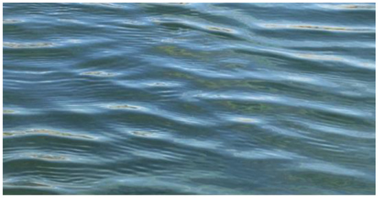
Figure 6. Interactions between two wave frequencies with equal phase speed. Wind: Light breeze towards the camera. Air temp.: 7 °C. Water temp.: 3 °C. $\lambda \left(\mathrm{capillary}\right) \approx 6 \mathrm{mm}$. $\mathsf{\lambda }\left(\mathrm{gravity}\right) \approx 5 \mathrm{cm}$. Fetch length $\approx$ 10 m. Behind the camera, waves with longer wavelengths grew.

According to [29], a laminar boundary layer develops below the surface in the early stage of an experiment when the wind speed grows. Hence, during this short period of time, $I$ and $V$ are most probably functions of $z$. Then, the dissipation is smaller than $D$ as given by (55), while $W_2$ and $W_3$, as given by (49) and (51), are valid. After a constant amplitude and current speed are reached, then (9) implies that $V^{\prime }=0$. Then $D$ from (55) is valid, and so is (56).

$W_{ex}$ seems to be the “energy transfer from the waves to the main flow” described in [30]. Under conditions like those shown in Figure 3, the main flow is provided by gravity waves. Therefore, $W_{ex}$ appears to be the energy transfer needed to obtain wave–wave interactions between wind-supported waves and waves at lower frequencies. Without it, since we found in Section 3.2 that gravity waves cannot grow by $W_1$ only, additional energy input is needed. However, with many frequencies and directions of the waves, the additional energy may come in many forms, and there is no reason to believe that results based on linear wave theory are generally valid. Hence, for gravity waves, $W_2$ is probably not required.

Visual observations have taught me that the wave-height of wind-supported waves seems to be near 1 mm (${\eta }_0\approx 0.5$ mm) for all wavelengths. With ${\eta }_0=0.5$ mm, $\lambda =$ 3.08 mm and $V=57$ s⁻¹, then $W_{ex}=$ 0.4 mW/m². Since the waves are fully grown, the excess energy must be transferred to other dynamics. Even if it is entirely transferred to waves at lower frequencies, it is far less than needed to explain the energy input to growing gravity waves under fresh breeze conditions. It may, however, supply energy to a lower frequency $\widehat{\omega }$. Then, the air pressure can transfer energy to growing gravity waves by $W_1\left(\widehat{\omega }\right)$, i.e., similar to (46) with ${\omega }_0$ replaced by $\widehat{\omega }, {\eta }_0$ by $\widehat{\eta }$ and $c_0$ by $\widehat{c}$.

In conclusion: while the main part of the energy input to growing gravity waves can be received directly by the air pressure’s work, some wind energy is transferred from capillaries to growing gravity waves. However, unless the gravity waves also accumulate angular momentum, no waves will appear. That problem is studied in Section 4.

4. Spin and Angular Momentum

4.1. Spin of Free Waves

Progressive water waves need angular momentum to exist, not only energy. It is a Lagrangian quantity, here denoted as spin to distinguish it from the angular momentum of other forms of dynamics, in particular currents. In [2], a formula is established for the spin of free, gravity waves with circular frequency $\widehat{\omega }$ and energy $E\left(\widehat{\omega }\right)$. In deep water, with the moment point at the mean water level, it is shown that the linear terms contribute to the spin vector with $\left(E/\widehat{\omega }\right)\mathit{j}$, while the second order Stokes drift adds a negative contribution $\left(-E/2\widehat{\omega }\right)\mathit{j}$. Hence the spin of regular, free gravity waves, correct to the second order, is

$$\mathit{S}\left(\widehat{\omega }\right)=\frac{E\left(\widehat{\omega }\right)}{2\widehat{\omega }}\mathit{j}.$$

(57)

Since $\mathit{S}$ is a horizontal vector, the total spin of a ring of waves, generated by a sphere that falls vertically into calm water, is zero. Ocean waves have a main direction of propagation and, therefore, spin. To amplify ocean waves, it is therefore not enough to add energy. Spin is also needed, and to amplify Stokes drift, so is momentum.

With many frequencies involved, a vector sum of the contributions from (57) gives the total spin of the waves. In the absence of external torques, it is shown in Appendix A that for linear, non-breaking, gravity waves, $\mathsf{\Sigma }\mathit{S}\left(\widehat{\omega }\right)$ is sufficiently constant over time to be treated as conserved. Hence, if dissipation reduces the wave energy, then some of the remaining wave energy is transferred to lower frequencies. Alternatively, or simultaneously, for waves with different propagation directions, the angle between the propagation directions can be reduced to obtain spin conservation.

Frequency downshifting is measured in laboratory experiments with nonbreaking waves in [31,32]. In [32], Figure 10 shows an experiment where the wave energy changes frequency from regular waves at 3.6 Hz to almost regular waves at 3.0 Hz over a distance of 9.1 m. In [4], Appendix A, it is shown that a full transfer between the two frequencies can be explained as a consequence of molecular dissipation and conservation of spin flux over a distance of 11 m. It implies that spin conservation, or in this case spin flux conservation, appears to be a useful tool. (The surface of the generated waves in [32] shows significant higher order amplitudes. Since the energy of the higher order terms is small compared to the linear contribution and the frequency needed to compute the $n$th order contribution is $n\widehat{\omega }$, the spin due to the higher order terms is sufficiently small to merely imply a small correction.)

In [33], the spin concept is developed further. It was found “that spin conservation lies behind nature’s invention of the thin topside breakers seen in laboratory, and in nature, to emerge from the very crests of breaking waves!”.

For free waves at any frequency, including gravity waves and capillaries, the wave energy $E\left(\widehat{\omega }\right)=\rho \widehat{\omega }c\left(\widehat{\omega }\right)\eta {\left(\widehat{\omega }\right)}^2/2$. Ref. Equation (33). When it is inserted in (57), then

$$\mathit{S}\left(\widehat{\omega }\right)=\frac{1}{4}\rho c\left(\widehat{\omega }\right)\eta {\left(\widehat{\omega }\right)}^2\mathit{j}.$$

(58)

It shows that a general consequence of reducing $\eta \left(\widehat{\omega }\right)$ by dissipation is energy transfer towards waves with higher speeds. Contrary to gravity waves, dissipation of capillaries therefore implies frequency upshifting. A similar result is obtained in [34] for capillaries by using fourth order wave theory. Equation (58) also allows dissipative interactions back and forth between gravity waves and capillaries as long as the phase speed of the receiving waves is bigger than that of the delivering waves.

Conservation of wave action [35] and spin [2] appear to be the same conservation theorem, since spin of gravity waves as given in (57) is the half of wave action. However, since wave action is conserved merely for the wave part of the motion, it is not useful here, as interactions with wind and currents are treated as well. Further, wave action conservation does not allow dissipation.

4.2. Input of Angular Momentum from the Wind

The conservation theorem of angular momentum is adopted on a system that consists of the water waves inside an imagined, rectangular box that is fixed in space. Its length is a whole number of wavelengths and its bottom is at a depth without motion. The moment point is located at the mean water level. Since the external forces on the system on the vertical boundaries are either constant and opposite or sinusoidal, their mean values are zero. Hence, the air causes all net external forces on the system, and only torques due to the wind add angular momentum. In addition, the wind may accelerate currents. This implies that the current’s negative angular momentum increases so that the spin of the waves increases to counteract the negative increase in angular momentum. Consequently, the total spin of the waves increases faster than given by the external torques.

There is no contribution to torques from the vertical component of the air pressure, since the pressure’s mean value over a wave period is the same everywhere. The moment of the horizontal component of the air pressure is $M=⟨\tilde{s}{\tilde{\eta }}_0{\tilde{p}}_{air}⟩$, where $\tilde{s}=\partial {\tilde{\eta }}_0/\partial x$ is the steepness of the surface. If ${\tilde{p}}_{air}$ is constant, $M=0$ because $\tilde{s}$ is a derivative of ${\tilde{\eta }}_0$. If ${\tilde{p}}_{air}$ is not constant, $M=0$ because it is a product of three harmonic functions. The only contributor to external torques is therefore the moment of the horizontal component of the viscous forces $M=\mu ⟨{\tilde{u}}^{\prime }{\tilde{\eta }}_0⟩$. By inserting from (4) and (T13),

$$M=\frac{1}{2}\mu k\left({\omega }_0-V\right){\eta }_0^2.$$

(59)

For wind-generated waves, gravity waves and capillaries are usually observed together. Then they share a common surface value of $V$. Gravity waves may therefore receive angular momentum from the wind, as well. To find the external torques on gravity waves with frequency $\widehat{\omega }$, wave number $k\left(\widehat{\omega }\right)$ and amplitude $\eta \left(\widehat{\omega }\right)$, (59) is rewritten to

$$\widehat{M}=\frac{1}{2}\mu k\left(\widehat{\omega }\right)\left(\widehat{\omega }-V\right)\eta {\left(\widehat{\omega }\right)}^2.$$

(60)

At the highest frequencies of gravity waves, where $\widehat{\omega }>V$, often $\eta \left(\widehat{\omega }\right)>{\eta }_0$, as well. Therefore, several gravity wave frequencies in the actual, high-frequency range may provide a significant additional input of angular momentum from the wind. Although, for a major part of the gravity waves, $\widehat{\omega }<V$. Hence, these frequencies depend on spin input from capillaries.

A consequence of this is that while wind energy is mainly transferred to growing gravity waves, the angular momentum is mainly transferred from the wind to capillaries. Figure 6 shows the consequence in an early phase of the wind-wave generation process.

With (1) as a basis, it follows from Table 2 that a wind speed of 9.75 m/s generates waves with $\mathsf{\lambda }=3.08$ mm. With ${\eta }_0=0.5$ mm at 20 °C, values from Table 2 imply that $M=$ 185 Nm/m², which, after 1 h, implies that the accumulated spin is 660 Nms⁻¹/m² and, after 10 h, 6.6 kNms⁻¹/m². Under similar wind conditions (20 knots), the nomogram 3–15 in [36] shows a significant wave height of 0.5 m and a significant period of 2.1 s after 1 h, and 1.7 m and a significant period of 5.3 s after 10 h. For regular waves, the spin of the two alternatives is 51 Nms⁻¹/m² and 1.5 kNms⁻¹/m², i.e., an order of magnitude smaller than the values obtained from (59). Hence, $M$, as given by (59), seems to provide enough spin to explain observed ocean waves. The contributions from $\widehat{M}$ and an accelerating current strengthen the conclusion.

The inaccuracy involved by comparing regular waves with wave spectra is deliberate. The approach is chosen, partly because the directional distribution varies throughout a spectrum, partly because the shape of the frequency spectrum varies, partly because the transfer of angular momentum between the waves and the current is unknown and partly because the capillaries travel in different directions and never cover the surface completely, as can be seen in Figure 3. In addition, the accuracy of the nomogram can be questioned. Therefore, little is gained by more elaborate evaluations.

4.3. Frequency Downshifting

When excess energy and spin leave the wind-supported waves and accumulate at one or more lower frequencies, it is the beginning of the general downshifting process. Then, spin and some energy must “travel” through the saturation range in order to accumulate in the growing peak. In addition to the measurements from [31,32], referred to in Section 4.1, frequency downshifting is reported in [1,37,38] and many others. A general conclusion is that when the wind speed increases, more whitecaps appear, and a faster growth of waves is observed. Hence, at a fresh breeze, more spin reaches the peak of the spectrum per minute than at lower wind speeds. So, while $W_1$ causes a major part of the energy input to growing waves at the peak, the required spin together with the remaining excess energy are provided through wave breaking and other dissipative processes throughout the saturation range. The consequences is studied in [2,4]. Then, merely what is here denoted excess energy was considered, while the need of energy input to the peak was not realized.

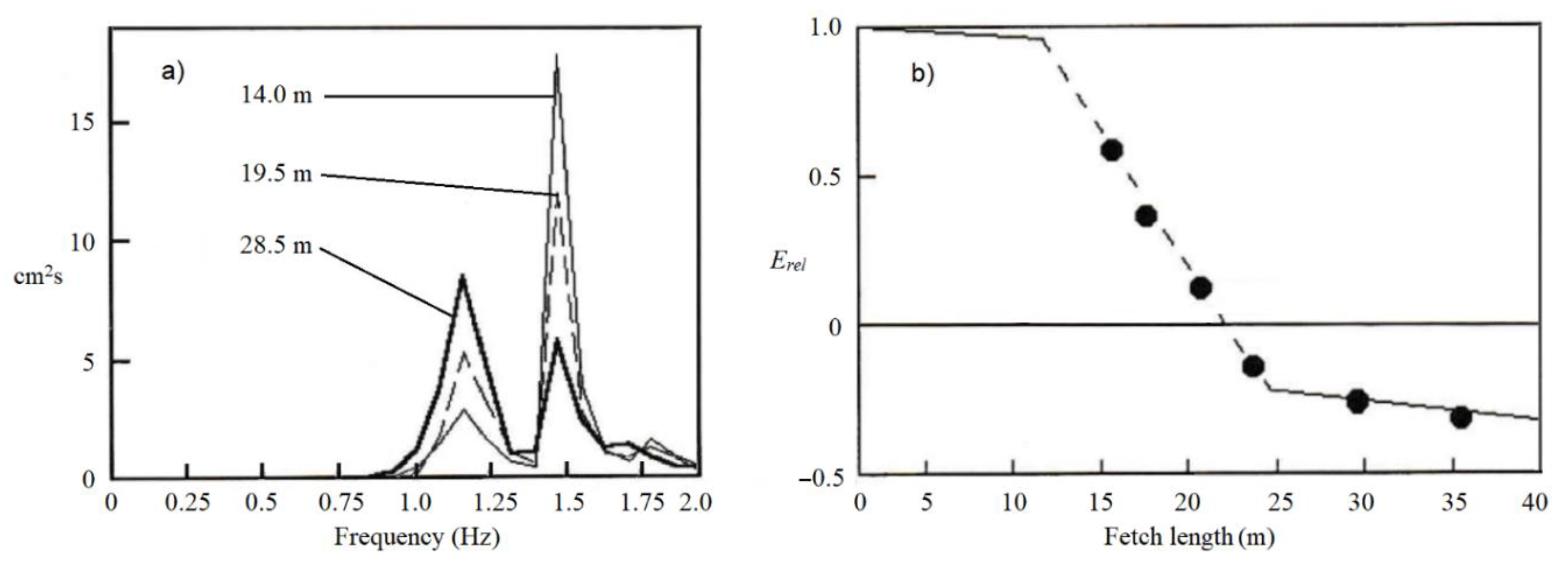
Figure 7 shows graphs of downshifting of deep water, initially steep, regular waves at a frequency of 1.5 Hz. As can be seen in Figure 7a, two sideband frequencies, known from [39] as non-dissipative phenomena (spin conservation needs both frequencies), grew until breaking occurred about 10 m from the wave generator. They grew until a variable wave height implied the start of wave breaking about 10 m from the wave generator. From there, wave breaking appeared over a distance of 13 m where much of the wave energy shifted to waves at 1.2 Hz. On Figure 7b, the two slightly tilted lines show the effect of molecular dissipation, while the dotted line shows the effect of wave breaking. It is about twenty times steeper than the two other lines and indicates that the dissipation in this case was an order of magnitude stronger than molecular dissipation.

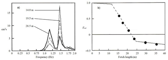
Figure 7. Downshifting of gravity waves. Generated frequency: 1.5 Hz. Intended wave height: 35 mm. Water temp.: 16 °C. In (b), $E_{rel}=\frac{\left(E_{1.5}-E_{1.2}\right)}{\left(E_{1.5}+E_{1.2}\right)}$, in which $E_{1.2}$ and $E_{1.5}$ are the wave energy below the peaks at 1.2 Hz and 1.5 Hz of the spectra, of which three are shown in (a). The measurements were performed simultaneously by five wave gauges in the Ocean Basin in Trondheim, Norway. (From [40]).

4.4. Swells

From field measurements shown in [37,38,41] and more than 20,000 observations in [42], it can be concluded that the wind does not amplify swells nor change their propagation direction. It is as expected from the present theory.

5. Conclusions

The theory for wind-supported waves appears to give a good description of such waves and their part of the wave generation process for wind speeds below 10 m/s or so. In particular, the wavelength is found to have a dependency on the wind speed that is similar to observations. However, since the capillaries at the highest frequencies are clearly nonlinear, the linear approach implies that calculated values should be used with care. Moreover, even if future measurements confirm that (1) is correct when the wind velocity is constant, variable wind conditions imply that significant deviations from (1) should be expected when the wind accelerates—as it usually does at sea. Even turbulence in the wind under laboratory conditions implies that a comparison between this theory and laboratory measurements should be treated carefully.

It is time to sum up other central results.

• Energy input from the wind is provided in three different ways by $W_1, W_2$ and $W_3$ as given by (46), (49) and (51).
• A consequence of (60) is that shear stresses provide input of angular momentum from the wind to the high-frequency parts of a spectrum only.
• Another consequence of (60) is that swells cannot grow when energy and spin input from other frequencies is missing.
• Without energy input by $W_2$ and $W_3$ to wind-supported capillaries, the ocean would have been mainly flat. Merely ship waves, tsunamis, etc. would exist.
• The air pressure cannot amplify gravity waves without input of energy and spin from other frequencies through wave–wave interactions. Refs. Equations (56) and (60).
• Spin conservation implies energy transfer to waves with higher phase speeds. Ref. Equation (58).
• It follows from (39) that wind-supported waves depend on the existence of laminar surface conditions, and that ${\omega }_0$ and $V$ are mutually dependent on each other.
• A shear current implies that the orbits of the water of linear waves are elliptic, where the horizontal axes are longer than the vertical axes when $V>0$. Ref. Equations (7), (16) and (38).
• It follows from Table 2 that the vorticity of the current determines the frequency of wind-supported waves.

What are not explained are:

○

Observed wave heights of wind-supported waves hardly exceed 1 mm.

○

If (1) is correct, then $V$ is not a function of the wind speed when the wind speed exceeds 10 m/s. It implies that the theory does not explain why increasing gales imply increasing wave growth.

References

- Tulin, M.P.; Waseda, T. Laboratory observations of wave group evolution, including breaking effects. J. Fluid Mech. 1999, 378, 197–232. [Google Scholar] [CrossRef]
- Naeser, H. Why ripples become swells and waves in shallow water decay rapidly. Geophys. Astrophys. Fluid Dyn. 1979, 13, 335–345. [Google Scholar] [CrossRef]
- Longuet-Higgins, M. Spin and angular momentum in gravity waves. J. Fluid Mech. 1980, 97, 1–25. [Google Scholar] [CrossRef]
- Naeser, H. A theory for the evolution of wind-generated gravity-wave spectra due to dissipation. Geophys. Astrophys. Fluid Dyn. 1981, 18, 75–92. [Google Scholar] [CrossRef]
- Grare, L.; Peirson, W.L.; Branger, H.; Walker, J.; Giovanangeli, J.-P.; Makin, V. Growth and dissipation of wind-forced, deep-water waves. J. Fluid Mech. 2013, 722, 5–50. [Google Scholar] [CrossRef]
- Caulliez, G. Dissipation regimes for short wind waves. J. Geophys. Res. Oceans 2013, 118, 682–684. [Google Scholar] [CrossRef]
- Shemdin, O.H. Wind-generated current and phase speed of wind waves. J. Phys. Oceanogr. 1972, 2, 411–419. [Google Scholar] [CrossRef]
- McLeish, W.L.; Putland, G.E. 1975 Measurements of wind-driven flow profiles in the top millimeter of water. J. Phys. Oceanogr. 1975, 5, 516–518. [Google Scholar] [CrossRef]
- Wu, J. Wind-induced drift currents. J. Fluid Mech. 1975, 68, 49–70. [Google Scholar] [CrossRef]
- Siddiqui, M.H.K.; Loewen, M.R. Characteristics of the wind drift layer and microscale breaking waves. J. Fluid Mech. 2007, 573, 417–456. [Google Scholar] [CrossRef]
- Miles, J.W. On the generation of waves by shear flows. J. Fluid Mech. 1957, 3, 185–204. [Google Scholar] [CrossRef]
- Miles, J.W. On the generation of waves by shear flows. Part 2. J. Fluid Mech. 1959, 6, 568–582. [Google Scholar] [CrossRef]
- Airy, G.B. Tides and waves. Encycl. Metrop. 1841, 11, 192. [Google Scholar]
- Longuet-Higgins, M. Parasitic capillaries: A direct calculation. J. Fluid Mech. 1995, 301, 79–107. [Google Scholar] [CrossRef]
- Melville, W.K.; Fedorov, A.V. 2015 The equilibrium dynamics and statistics of gravity-capillaries. J. Fluid Mech. 2015, 767, 449–466. [Google Scholar] [CrossRef]
- Gibbs, J.W. On the equilibrium of heterogeneous substances. Part II. Trans. Conn. Acad. Arts Sci. 1878, 3, 343–524. [Google Scholar]
- Franklin, B.; Brownrigg, W.; Farish, M. On the stilling of waves by means of oil. R. Soc. 1774, 12, 445–459. [Google Scholar]
- Jeffreys, H. On the formation of water waves by wind. Proc. R. Soc. A 1925, 107, 189–206. [Google Scholar]
- Jeffreys, H. On the formation of water waves by wind II. Proc. R. Soc. A 1925, 110, 341–347. [Google Scholar]
- Thompson, P.D. The propagation of small surface disturbances through rotational flow. Ann. N. Y. Acad. Sci. 1949, 51, 463–474. [Google Scholar] [CrossRef]
- Abdullah, A.J. Wave motion at the surface of a current which has an exponential distribution of vorticity. Ann. N. Y. Acad. Sci. 1949, 51, 425–441. [Google Scholar] [CrossRef]
- Valenzuela, G.R. The growth of gravity-capillaries in the coupled shear flow. J. Fluid Mech. 1976, 76, 229–250. [Google Scholar] [CrossRef]
- Kawai, S. Generation of initial wavelets by instability of a coupled shear flow and their evolution to wind waves. J. Fluid Mech. 1979, 93, 661–703. [Google Scholar] [CrossRef]
- Plant, W.J.; Wright, J.W. Phase speeds of upwind and downwind travelling short gravity waves. J. Geophys. Res. 1980, 85, 3304–3310. [Google Scholar] [CrossRef]
- Van Gastel, K.; Janssen, P.A.E.M.; Komen, G.J. On phase velocity and growth rate of wind-induced gravity-capillaries. J. Fluid Mech. 1985, 161, 199–216. [Google Scholar] [CrossRef]
- Kinsman, B. Wind Waves—Their Generation and Propagation on the Ocean Surface; Prentice-Hall: Englewood Cliffs, NJ, USA, 1965. [Google Scholar]
- Lamb, H. Hydrodynamics, 6th ed.; Cambridge University Press: Cambridge, UK, 1932. [Google Scholar]
- Bachelor, G.K. An Introduction to Fluid Dynamics; Cambridge University Press: Cambridge, UK, 1974. [Google Scholar]
- Melville, W.K.; Shear, R.; Veron, F. Laboratory measurements of the generation and evolution of Langmuir circulations. J. Fluid Mech. 1998, 364, 31–58. [Google Scholar] [CrossRef]
- Cheung, T.K.; Street, R.L. The turbulent layer in the water at an air-water interface. J. Fluid Mech. 1988, 194, 133–151. [Google Scholar] [CrossRef]
- Lake, B.M.; Yuen, H.C.; Rungaldier, H.; Ferguson, W.E. Nonlinear deep-water waves: Theory and experiment. Part 2. Evolution of a continuous wave train. J. Fluid Mech. 1977, 83, 49–74. [Google Scholar] [CrossRef]
- Lake, B.M.; Yuen, H.C. Model for nonlinear wind waves: Part 1. Physical model and experimental evidence. Evolution of a continuous wave train. J. Fluid Mech. 1978, 88, 33–62. [Google Scholar] [CrossRef]
- Tulin, M.P. Breaking of ocean waves and downshifting. In Waves and Nonlinear Processes in Hydrodynamics; Grue, J., Gjevik, B., Weber, J.E., Eds.; Kluwer Academic Publishers: Dordrecht, The Netherlands; Boston, MA, USA; London, UK, 1996; pp. 177–190. [Google Scholar]
- Hara, T.; Mei, C.C. Wind effects on the nonlinear evolution of slowly varying gravity-capillary waves. J. Fluid Mech. 1994, 267, 221–250. [Google Scholar] [CrossRef]
- Bretherton, F.P.; Garret, C.J.R. Wavetrains in inhomogeneous moving media. Proc. R. Soc. Lond. A 1968, 302, 529–554. [Google Scholar]
- Coastal Engineering Research Center (US). Shore Protection Manual, 3rd ed.; U.S. Army Corps of Engineer, Coastal Engineer Research Center: Vicksburg, MS, USA, 1977. [Google Scholar]
- Snodgrass, F.E.; Growe, G.W.; Hasselmann, K.F.; Miller, G.R.; Munk, W.H.; Powers, W.H. Propagation of ocean swell across the Pacific. Philos. Trans. 1966, 259, 431–497. [Google Scholar]
- Hasselmann, K.; Barnett, T.B.; Bouws, E.; Carlson, H.; Cartwright, D.E.; Enke, K.; Ewing, J.A.; Gienapp, H.; Hasselmann, D.E.; Kruseman, P.; et al. Measurements of wind-wave growth and swell decay during the Joint North Sea Wave Project. Ergänzungsheft Zur Dtsch. Hydrogr. Z. 1973, 8, 12. [Google Scholar]
- Benjamin, T.B.; Feir, J.E. The disintegration of wave trains on deep water Part 1. Theory. J. Fluid Mech. 1967, 27, 417–430. [Google Scholar] [CrossRef]
- Naeser, H. Energy accumulation in ocean waves. Proc. 3rd Eur. Wave Energy Conf. 1998, 2, 296–303. [Google Scholar]
- Mitsuyasu, H. Measurements of high-frequency spectrum of ocean surface waves. J. Phys. Ocean. 1977, 7, 882–891. [Google Scholar] [CrossRef]
- Torsethaugen, K. A two peak wave spectrum model. OAME—II Safety and reliability. ASME 1993, 175–180. [Google Scholar]
- Naeser, H. Conservation of partial angular momentum with applications on water waves. J. Appl. Sci. 2002, 2, 682–685. [Google Scholar]
Publisher’s Note: MDPI stays neutral with regard to jurisdictional claims in published maps and institutional affiliations. |
© 2022 by the author. Licensee MDPI, Basel, Switzerland. This article is an open access article distributed under the terms and conditions of the Creative Commons Attribution (CC BY) license (https://creativecommons.org/licenses/by/4.0/).