Reducing Slipstream Velocities Experienced in Proximity to High-Speed Trains

Abstract

Slipstream wake structures generated by the passing of high-speed rail vehicles represent a hazard to passengers and workers in close proximity. In this article, the possibility of reducing peak slipstream velocities through the implementation of angled fins or swirling flow injection is assessed on the basis of improved delayed detached eddy simulations (IDDES). The key to improving slipstream velocities involves redirecting and/or reducing the internal energy, a pair of meandering counter-rotating vortex cores that are associated with large wake slipstream deviations. It is demonstrated that the danger imposed by slipstream wake structures, as measured by the induced velocity measures recorded at a series of test points adjacent to the passing train, could be significantly reduced, with decreases from 10% up to 23%, recorded across a range of sampling locations. The means by which these reductions are generated and the corresponding changes in the flow are also explored through analysis of the modified wakes. As such, these devices show promise at improving the operational safety of high-speed rail vehicles.

1. Introduction

A high-speed train is generally regarded to be a rail vehicle that spends a significant portion of its travel time at velocities over 200 km/h, although speeds can be significantly greater than this. At such extreme speeds, train geometry is not only key in minimizing drag, but also in managing the generation of large slipstream flow structures that arise in the wake of these vehicles as they travel. Slipstream flows are defined (Bell et al. [1]) as “the air flow induced by the train’s movement as experienced by a stationary observer”. High induced velocities can extend out to a sufficient spanwise distance from the tracks, so as to pose a safety risk to people located in close proximity to passing trains, most commonly commuters waiting at stations and track-side workers. This is addressed in Baker et al. [2], where it was suggested that gust speeds as low as 15 m/s could be sufficient to cause people to “stumble or be displaced”. The slipstream behaviour of high-speed trains is hence of great interest from an operational perspective.

This study follows previous extensive wind-tunnel testing programmes conducted at Monash University on scale models of the ICE-2 and ICE-3 (Inter-City Express 2 and 3) high-speed trains. Recent work (Bell et al. [1], Bell et al. [3] and Bell et al. [4]) focused on analysing the characteristics of high-speed train wake profiles in considerable depth, and examined the spanwise oscillation of the time-mean counter-rotating trailing vortex pair as a leading cause of large slipstream disturbances in the wake (that extend beyond the width of the train). In a later study, Bell et al. [5] explored large-scale redesigns of the tail geometry as a means of slipstream control. It was observed that by increasing the angle at which the tail section diverged from the train body, so as to generate a shorter/blunter tail section, slipstream velocities could be potentially reduced, but at the cost of increased pressure drag. That study identified that the most streamlined designs didn’t necessarily result in the smallest slipstream velocities, and suggested that there may be a better compromise between reducing slipstream measures and increasing the drag force experienced by the train. This was also explored more recently in Chen et al. [6], where the nose length of a high-speed train model was altered to reduce recorded slipstream velocities.

This study builds on the work of Wang et al. [7], in which a computational model of a high-speed train wake was demonstrated to satisfactorily reproduce experimental wind-tunnel results of Bell et al. [4]. Using the validated model developed by Wang et al. [7] as a baseline, the aim of this investigation was to determine whether implementing different flow control techniques onto a ICE-3 train model could feasibly reduce recorded slipstream velocities.

Work by Muld [8], Bell et al. [3] and Bell et al. [4], as alluded to above, identified that a dominant feature of the time-mean wake topology of high-speed trains is a counter-rotating trailing vortex pair. This is generated as the flow rolls downwards from each side of the train at the tail, redirecting boundary-layer vorticity into streamwise-aligned vorticity of the pair. Moreover, the streamwise vortices of the pair oscillate across the wake as they advect downstream and large instantaneous excursions occur, causing higher velocity fluid to be transported a considerable cross-stream distance from the train centreline. Thus, the control methods studied here focused on controlling or manipulating this vortex-pair wake structure as a way to control wake slipstream development.

2. Methodology

The high-speed train geometry used in this study is the same as that employed in Wang et al. [7]: a simplified single-carriage replication of a Deutsche Bahn Inter-City Express 3 or ICE-3 high-speed train with a length-width-height ratio of approximately 50:3:4, compared to a general configuration of 200:3:4. The reduction in relative length was to keep computational costs under control, with an estimated reduction in computational run-time of a factor of 4 and the required memory a factor of 2.5. The train is placed on a single-track ballast and rail ground configuration. This layout is shown in Figure 1.

The ground surface was flat, and no crosswind was present. The inlet of the domain was one train length forward of the nose of the model, and the outlet was positioned three train lengths from the tail of the train. This distance allows for slipstream structures to develop and persist sufficiently far downstream so that the maximal slipstream velocities along set measurement lines are recorded well before the wake reaches the outlet. This was verified through additional simulations using longer domains in Dunlop [9]. All designs were tested subject to a moving floor condition; therefore, in this frame of reference, the surfaces that constitute the train model remain stationary, while the flow moves past the train at the specified inlet velocity with matching linear translational motion of the ground, ballast and rail surfaces. The width and height of the domain are 40 and 20 train widths, respectively, yielding a blockage ratio of 0.17%. In the following, the width of the train is used as the reference length ($L_{Ref}$).

The investigation was conducted using ANSYS FLUENT V19.2 at a Reynolds number of 720,000, matching the scale-model wind-tunnel studies of Bell et al. [1], Bell et al. [3]. and Bell et al. [4], although this is considerably lower than a typical operational Reynolds number of approximately 20,000,000. A constant velocity was used at the inlet, and a turbulence intensity of 1% was applied, which is typical of turbulence levels of wind-tunnel facilities. The outlet was defined as a zero pressure outlet, and with zero-gradient velocity components, i.e., $d\overrightarrow{u}/d\overrightarrow{n}\equiv \overrightarrow{n}·\nabla \overrightarrow{u}=0$, with $\overrightarrow{n}$ the outflow surface normal. The flow state was initialised using FLUENT hybrid initialisation.

On the basis of successful simulations for the ICE-3 high-speed train base model presented in Wang et al. [7], an improved delayed detached eddy simulation (IDDES) turbulence model incorporating the shear-stress transport (SST) k–$\omega$ Reynolds-Averaged Navier–Stokes (RANS) model for near-wall zones was used for all simulations reported here. Essentially, the IDDES model uses large-eddy simulation (LES) away from boundaries and blends this with a RANS simulation of near-wall regions. This approach is a development of the delayed eddy simulation (DES) method originally proposed by Spalart et al. [10] used to model separated flows.

The SST k–$\omega$ turbulence model employed for the RANS component of the IDDES model is defined as follows, partially symbolically; k is the turbulent kinetic energy per unit mass, and $\omega$ is the specific dissipation rate.

$$\frac{\partial }{\partial t}\left(\rho k\right)+\frac{\partial }{\partial x_j}\left(\rho k{\overline{u}}_j\right)=P_k-{\beta }^{*}\rho k\omega +\frac{\partial }{\partial x_j}\left((\mu +\frac{{\mu }_T}{{\tilde{\sigma }}_k})\frac{\partial k}{\partial x_j}\right)$$

(1)

$$\frac{\partial }{\partial t}\left(\rho \omega \right)+\frac{\partial }{\partial x_j}\left(\rho \omega {\overline{u}}_j\right)=\tilde{\alpha }\frac{\omega }{k}{P}_k-\tilde{\beta }\rho {\omega }^2+(1-F_1)\rho \frac{2}{{\sigma }_{\omega }}\frac{\partial k}{\partial x_j}\frac{\partial \omega }{\partial x_j}+\frac{\partial }{\partial x_j}\left((\mu +\frac{{\mu }_T}{{\tilde{\sigma }}_{\omega }})\frac{\partial \omega }{\partial x_j}\right)$$

(2)

In this case, the turbulent viscosity is given by ${\mu }_T=\rho k/\omega$ for the standard k–$\omega$ model. There are recognisable terms here: the local rate of change (1st term); the advective rate of change (2nd term); and molecular and turbulent diffusion (last terms) for both k and $\omega$. There are also terms representing turbulent kinetic energy production ($P_k$) and dissipation (${\beta }^{*}\rho k\omega$), with similar terms in the specific dissipation equation.

The remaining term ($(1-F_1)\rho \frac{2}{{\sigma }_{\omega }}\frac{\partial k}{\partial x_j}\frac{\partial \omega }{\partial x_j}$) switches between the k–$\omega$ model near the wall and the k–$ϵ$ equation further away, taking into account the strengths of each model to treat flow over different parts of the flow domain. Function $F_1$ is a blending function to switch between these modes. In addition, the SST model adjusts the turbulent viscosity so that it obtains the correct physical behaviour in adverse pressure gradient regions, where the standard approach results in delayed separation. Thus, the SST k–$\omega$ model gives improved prediction of separation in adverse pressure gradients, which is certainly a useful feature for predicting separation towards the rear for a streamlined high-speed train.

The key factor in the success or otherwise of DES modelling is determining when to switch between the RANS and LES models at the edge of the boundary layer. This is typically determined by a modified length scale $d_{\mathrm{D}\mathrm{E}\mathrm{S}}$ that is dependent on the distance to the closest point on the wall (d), an empirical constant ($C_{\mathrm{D}\mathrm{E}\mathrm{S}}$) of 0.65, and the maximal local cell size (${\Delta }_{\mathrm{m}\mathrm{a}\mathrm{x}}$), with $d_{\mathrm{D}\mathrm{E}\mathrm{S}}=min(d,C_{\mathrm{D}\mathrm{E}\mathrm{S}}·{\Delta }_{\mathrm{m}\mathrm{a}\mathrm{x}})$. Delayed DES (DDES) varies this length scale by adding a shielding function ($f_d$) to ensure that LES is not activated within the boundary layer:

$$d_{\mathrm{D}\mathrm{D}\mathrm{E}\mathrm{S}}=d-f_d·max(0,d-C_{\mathrm{D}\mathrm{E}\mathrm{S}}·{\Delta }_{\mathrm{m}\mathrm{a}\mathrm{x}})$$

(3)

Lastly, IDDES introduces wall-modelled LES (WMLES), which allows for the outer regions of a boundary layer to be solved using LES when the grid resolution is sufficient, while DDES is employed when it is not. The full details of the IDDES method are provided in the following references: Shur et al. [11], Gritskevich et al. [12] and Saini et al. [13], with the implementation in ANSYS FLUENT presented in [14].

The iterative time-stepping approach was used to evolve the flow with up to 30 inner iterations per time step. The time step was selected on the basis of the results of Wang et al. [7], where minimal variation was observed in slipstream and drag predictions when the time step was varied by an order of magnitude between 0.025 and 0.0025$T_{ref}$. As such, a time step of 0.033$T_{ref}$ was selected, and this time step size is equivalent to the 0.025$T_{ref}$ value presented in Wang et al. [7], as that study used the height rather than width of the vehicle as the reference length, and switching to width allowed for more near wake points to be sampled as simple functions of the reference length. A sampling period of 600$T_{ref}$ was utilised for the collection of data presented below. This equates to the fluid passing the train approximately 36 times.

The computational meshes utilised in the current study were modifications of that presented in Wang et al. [7] (see Appendix A for further details) adjusted to improve mesh resolution in proximity to control devices; specifically, significantly increased cell concentration was added in the vicinity of and surrounding control devices. These regions extended 1$L_{Ref}$ upstream, 2$L_{Ref}$ downstream, and 0.5$L_{Ref}$ in the spanwise and vertical directions from the extremities of each device. The element size within these regions was 1/60 $L_{Ref}$. All control devices also had reduced element sizing, with a face sizing of 1/120$L_{Ref}$ and a reduced inflation layer growth rate of 1.1 compared to surrounding regions. The other key alteration to the mesh presented in Wang et al. [7] was an increase in the size of the “train body” body of influence, which was increased in length from 25 to 51.66$L_{Ref}$, and in height from 2 to 2.66$L_{Ref}$, as preliminary testing presented in Dunlop [9] indicated that significant high-velocity wake excursions were occurring outside the original high-resolution wake region when the control devices were added. The resulting meshes contained between 28 and 32 million cells, dependent on the complexity of the added control device.

Within the research presented in Dunlop [9], 83 different devices were evaluated for their ability to modify and control the slipstream flow. This paper explores in detail the two most promising concepts that arose on the basis of the ability to reduce recorded slipstream velocity measures at common bystander locations.

The parallel fins were a pair of surface modifications applied to the rear of the train geometry, with the intent to shift the counter-rotating vortex cores towards one side of the model. This was expected to reduce the intensity of slipstream velocities on the other side of the model, termed the passenger side, while potentially increasing slipstream velocities on the side towards which the flow was redirected, termed the danger side. The fins were positioned on the downwards slope of the rear of the train geometry, with a flat upper surface emerging smoothly from the train geometry at a distance 15.33$L_{Ref}$ downstream from the nose of the train, a steady height of 1.5$L_{Ref}$ above the floor and extending 1.25$L_{Ref}$ downstream (when no deflection angle was applied), until ceasing at a right angle down to the surface of the initial geometry. The fins were 1/120$L_{Ref}$ thick and had a base spanwise displacement of 1/8$L_{Ref}$ from the centre-plane, placing the pair of fins 1/4$L_{Ref}$ apart before the deflection was applied around the centre-point. For the case presented in the results section, this rotation was 7 degrees in magnitude. A rear view of this device is seen in Figure 2a, while Figure 2c shows a side view of the fins prior to rotation.

The second means by which the flow was altered was through the injection of swirling flow at the tail of the train, with the intention of counteracting the circulation generated by the counter-rotating vortex core pair that formed in the baseline train wake. To achieve this, a set of flow injection regions were generated at the tail of the train, defined by the intersection of cylinders projected in the stream-wise direction. Each cylinder was centred at a point 1$L_{Ref}$ above the ground, 1/4$L_{Ref}$ from the centre-plane in the spanwise direction and with a diameter of 1/5$L_{Ref}$. These circulating flow injection ports are illustrated in Figure 2b.

The intent behind this design was not to inject flow at a significantly greater velocity than the surrounding flow, as the primary variable of interest was the circulation of the injected flow. However, too-low injection velocity would result in circulation failing to consistently propagate downstream. In the preliminary testing of Dunlop [9], streamwise injection velocities were tested with no added circulation to establish an injection velocity which matched the baseline flow in the near wake to within 2%. As a result of this testing, a speed of 5/7$U_{Inlet}$ was selected for all cases. In an attempt to cancel or control the naturally present vortex structures, the direction of the injected circulation was reversed across the spanwise symmetry plane. For all cases investigated the radial velocity of the flow from the injection port was set as zero and a turbulence intensity of 5% and a turbulent viscosity ratio of 10 utilised, noting that the predictions are unlikely to be strongly affected by the exact values chosen. After varying the circulation intensity, by modifying the tangential velocity of the injected flow from 0 to 1/2$U_{Inlet}$, 2/7$U_{Inlet}$ was observed to produce the greatest reduction in the recorded slipstream velocity measures. As such, this is the value used for results presented below. The full results of these preliminary tests can be found in Dunlop [9].

To quantify the effect of the control devices, three parameters are discussed: near-wake x vorticity, the proper orthogonal decomposition (POD) of the slipstream velocity in downstream cross-planes, and the slipstream velocity measures along the test lines. The near wake x-vorticity is the time-averaged vorticity restricted to a plane perpendicular to the streamwise direction, to provide a clear visual indication of the effect on the intensity and location of the counter-rotating vortex cores.

The dataset used in POD analysis was that of the slipstream velocity at eleven vertical planes from 2 to 12$L_{Ref}$ downstream of the train rear. The deconstruction employed the approach defined in Kutz et al. [15]. Each plane for which POD data were exported extended 2$L_{Ref}$ in both spanwise directions from the centre plane, and 8/3$L_{Ref}$ vertically from the ground, although when presented visually, this area was trimmed to focus on regions with noticeable variation.

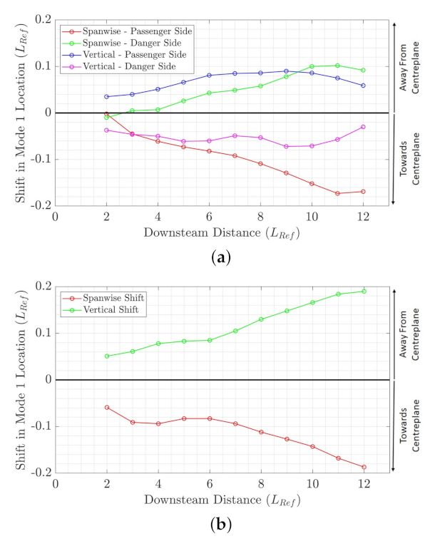
This analysis was utilised for obtaining mean slipstream velocity fields, to produce differential profiles from the unmodified baseline case, and to illustrate the variation in energy and location of the highest-order mode (or mode 1) of the slipstream velocity, which had been shown to be a strong indicator of the counter-rotating vortex cores. An example of a mean and mode 1 profile is shown in Figure 3 for the baseline case.

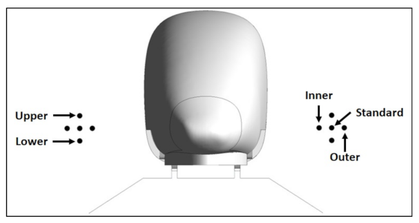
To obtain slipstream velocity measure data, five sample lines were generated running from the inlet to the outlet on each side of the train. The standard lines were positioned 1$L_{Ref}$ from the centre plane of the model and 0.4$L_{Ref}$ above the platform on both sides of the train, while each of the other four lines were positioned a distance of 0.1$L_{Ref}$ in either the spanwise or vertical direction from these standard lines. These locations are shown in Figure 4.

By convention, the vertical (z) velocity component was not used in the calculation of the slipstream velocities. It is defined by

$$U_{Slipstream}=\sqrt{{(U_{Ref}-u_x)}^2+u_y^2}$$

where $u_x$ and $u_y$ are the streamwise and spanwise velocity components measured in the train’s frame of reference. The measure of slipstream velocity for each pair of lines was generated by recording the maximum velocity at the conclusion of each time-step, taking the mean of this sample and adding two standard deviations. When presented graphically, an error bar indicating a 99.7% confidence interval was applied on the basis of the convergence of data from a wider variety of designs than tat presented in this paper Dunlop [9].

3. Results

3.1. Near-Wake x-Vorticity

The x-vorticity of the flow in the near wake is shown in Figure 5. The first shown case is that of the parallel fins, on the right-hand side of the figure. The baseline case is shown on the left for comparison.

In comparison to the baseline, at 0.1$L_{Ref}$ upstream of the tail (Figure 5a), the moderate-intensity region surrounding the vortex core on the passenger side (right side) grew significantly and was shifted towards the centre plane and further from the ground. On the danger side (left side), the region was elongated and began moving lower and further from the centre plane down the side of the tail. There was also a clear region of high vorticity extending downstream from the direct wake of the fins.

Further downstream at 1$L_{Ref}$ downstream of tail (Figure 5b), the passenger side region grows in size and moves further towards the danger side, separating the two regions of negative vorticity. The initial danger side core was significantly reduced in size, while the fin wake region continued to move lower and further towards the danger side, maintaining its intensity and dissipating less than the base vortex-core regions. As shown in subsequent analysis, the change in vorticity distribution affects the core locations relative to the vertical centre plane as the cores advected further downstream.

For the rear circulation injection shown in Figure 6, the counteracting circulation can be clearly observed in Figure 6a, where it dramatically disrupted the naturally present vortex cores. The effect of this further downstream is seen in Figure 6b, where the magnitude of the vorticity within the vortex cores was reduced, but more small-scale vorticity was present higher above the ground.

3.2. Slipstream Velocities

3.2.1. Mean Slipstream Velocity Fields

To further visualise the effect of the devices on the wake, the difference in the mean slipstream velocities in comparison to the baseline at a downstream distance of 3$L_{Ref}$ is shown in Figure 7.

For Figure 7a, the regions of increased velocity appear to show the new locations of the vortex-core structures after redirection by the fins. On the passenger side (left of image), it can be seen that the structure appears to be shifted higher and towards the centre plane, while on the danger side, no clear shift is apparent, only an increase in slipstream velocity.

For the circulation injection of Figure 7b, the profile was symmetrical, and the peak magnitude of the differentials was slightly reduced. However, there were clear reductions at the location of the vortex cores for the baseline train and a pair of regions of increased energy higher above the floor and closer to the centre plane. This matches with the x-vorticity observations of reduced energy close to the ground, but an increase in energy higher up.

3.2.2. POD: Mode 1 Slipstream Velocity Location

The primary mode of slipstream velocity is indicative of the counter-rotating vortex cores. As such, the spanwise and vertical shifts in the location of this mode when compared to the baseline case is of significant interest.

For both devices clear shifts are observed in the spanwise and vertical directions. For the parallel fins, Figure 8a shows the location of the mode is clearly shifted towards the centreplane on the passenger side and away from the centre plane on the danger side, with the extent of these shifts increasing with downstream distance. There was also a noticeable vertical shift further from the ground on the passenger side and towards the ground on the danger side, although these varied less with downstream distance.

The circulation injection wake is symmetrical, so the average of both sides can be taken. As seen in Figure 8b, the mode 1 location is shifted towards the centre plane in the spanwise direction to a similar magnitude to the parallel fins, while the height of the mode increases in an almost identical manner, indicating an almost perfectly diagonal shift in location.

3.2.3. POD: Mode 1 Slipstream Velocity Energy

The energy contained within the slipstream mode 1 was also a key consideration; thus, values were compared to the unmodified baseline case in Figure 9.

Disruptions to the vortex core formation seen in Figure 5 and Figure 6 appeared to reduce the energy present within these structures, with the circulation injection producing a reduction of nearly 50% in energy of the mode at a downstream distance of 3$L_{Ref}$ and a minimal reduction of 25%. While the reduction is less dramatic for the parallel fins at between 10–20%, it is still considerable, and indicates that these fins may have benefits aside from the spanwise redirection of the vortex cores.

3.2.4. Slipstream Velocity Measures

The final performance metric is the measure of slipstream velocity recorded at the five test locations; standard (i), upper (ii), lower (iii), inner (iv) and outer (v) (see Figure 4). For each case, red symbols indicate the test case, and black symbols the corresponding value for the baseline.

It is apparent from Figure 10 that both devices are capable of significant reductions in the recorded slipstream velocities at a range of locations. On the passenger side of the parallel fins model (Figure 10a), these reduction ranged from 10% for the upper line to 23% for the inner line. For the circulation injection of Figure 10c these reductions were marginally less dramatic, recording a minimum of 10% for the upper and outer lines, and a maximum of 17% for the inner line; however, this improvement was present on both sides of the train. The danger side of the parallel fins model, Figure 10b, was relatively neutral when compared to the baseline, with only a single location, the outer line, returning a greater measure than the baseline. This indicates that, while the slipstream velocities were only reduced on a single side of the model, there is not a significant increase in the intensity on the opposing side as anticipated.

4. Discussion

The results presented above indicate that both devices are capable of reducing recorded slipstream velocities around a high-speed train. It appears that the key to the success of both devices is the ability to redirect and reduce the intensity of the counter-rotating vortex core structures.

For the parallel fins, a clear trend of relocating high intensity flow regions away from the passenger side and towards the danger side was observed, making it less likely for large flow excursions to reach the test locations on this side of the model. This was the expected effect of this device, but these fins also proved effective at reducing the energy contained within the vortex cores, as represented by the mode 1 slipstream energy. This explains the unexpected neutral results recorded on the danger side of the parallel fins model, as, while the structures were shifted further in this direction, their intensity was reduced by the disruption generated by the fins.

The shift in the location of intense flow regions for the circulation devices is clearly illustrated by multiple metrics, with the interruption of the vortex core formation generating a dramatic shift further above the ground, and more importantly, closer to the centre plane. Combined with the dramatic mode 1 slipstream velocity energy reductions, it is no surprise that the slipstream measures are consistently reduced.

All of these results suggest that both devices may be capable of improving bystander safety, and are worth further exploration, potentially through experimental wind-tunnel testing or full-scale investigations.

References

1. Bell, J.R.; Burton, D.; Thompson, M.C.; Herbst, A.H.; Sheridan, J. Wind tunnel analysis of the slipstream and wake of a high-speed train. J. Wind Eng. Ind. Aerodyn. 2014, 134, 122–138. [Google Scholar] [CrossRef]
2. Baker, C.; Sterling, M.; Figura-Handy, G.; Johnson, T.; Free, P.; Munley, G.; Bowman, I.; Pope, C.; Gawthorpe, R. The Effect of Train Slipstreams on Passengers and Trackside Workers; Technical Report; Rail Safety and Standards Board Ltd.: Birmingham, UK, 2006. [Google Scholar]
3. Bell, J.R.; Burton, D.; Thompson, M.C.; Herbst, A.H.; Sheridan, J. Flow topology and unsteady features of the wake of a generic high-speed train. J. Fluids Struct. 2015, 61, 168–183. [Google Scholar] [CrossRef]
4. Bell, J.R.; Burton, D.; Thompson, M.C.; Herbst, A.H.; Sheridan, J. Dynamics of trailing vortices in the wake of a generic high-speed train. J. Fluids Struct. 2016, 65, 238–256. [Google Scholar] [CrossRef]
5. Bell, J.R.; Burton, D.; Thompson, M.C.; Herbst, A.H.; Sheridan, J. The effect of tail geometry on the slipstream and unsteady wake structure of high-speed trains. Exp. Therm. Fluid Sci. 2017, 83, 215–230. [Google Scholar] [CrossRef]
6. Chen, G.; Li, X.; Liu, Z.; Zhou, D.; Wang, Z.; Liang, X.; Krajnovic, S. Dynamic analysis of the effect of nose length on train aerodynamic performance. J. Wind Eng. Ind. Aerodyn. 2019, 184, 198–208. [Google Scholar] [CrossRef]
7. Wang, S.; Bell, J.R.; Burton, D.; Herbst, A.H.; Sheridan, J.; Thompson, M.C. The performance of different turbulence models (URANS, SAS and DES) for predicting high-speed train slipstream. J. Wind Eng. Ind. Aerodyn. 2017, 165, 46–57. [Google Scholar] [CrossRef]
8. Muld, T.W. Slipstream and Flow Structures in the Near Wake of High-Speed Trains; Technical Report; Royal Institute of Technology: Stockholm, Sweden, 2012. [Google Scholar]
9. Dunlop, J. Slipstream Control for High-Speed Trains. Ph.D. Thesis, Monash University, Clayton, Australia, 2021. [Google Scholar]
10. Spalart, P.R.; Jou, W.H.; Strelets, M.; Allmaras, S.R. Comments on the feasibility of LES for wings, and on a hybrid RANS/LES approach. In Advances in DNS/LES; Greyden Press: Columbus, OH, USA, 1997; pp. 137–147. [Google Scholar]
11. Shur, M.L.; Spalart, P.R.; Strelets, M.K.; Travin, A.K. A hybrid RANS-LES approach with delayed-DES and wall-modelled LES capabilities. Int. J. Heat Fluid Flow 2008, 29, 1638–1649. [Google Scholar] [CrossRef]
12. Gritskevich, M.S.; Garbaruk, A.V.; Schütze, J.; Menter, F.R. Development of DDES and IDDES formulations for the k-ω shear stress transport model. Flow, Turbul. Combust. 2012, 88, 431–449. [Google Scholar] [CrossRef]
13. Saini, R.; Karimi, N.; Duan, L.; Sadiki, A.; Mehdizadeh, A. Effects of near wall modeling in the improved-delayed-detached-eddy-simulation (IDDES) methodology. Entropy 2018, 20, 771. [Google Scholar] [CrossRef] [PubMed] [Green Version]
14. ANSYS. Ansys Fluent Theory Guide; ANSYS Inc.: Canonsburg, PA, USA, 2021. [Google Scholar]
15. Kutz, J.N.; Brunton, S.L.; Brunton, B.; Proctor, J.L. Dynamic Mode Decomposition; Society for Industrial and Applied Mathematics: Philadelphia, PA, USA, 2016; pp. 1–33. [Google Scholar]
Figure 1. Dimensions and layout of the computational model.
Fluids 07 00072 g001
Figure 2. Rear views of (a) parallel fins at seven degree orientation angle and (b) circulation injection vents. (c) Side view of fins before rotation is applied.
Fluids 07 00072 g002
Figure 3. POD (proper orthogonal decomposition) breakdown of slipstream velocity showing (a) the shape of the mean and (b) the highest order mode or mode 1 for the baseline train case at a downstream distance of 3 L R e f .
Fluids 07 00072 g003
Figure 4. Location of five sample lines on each side of the train.
Fluids 07 00072 g004
Figure 5. Mean x–vorticity comparison of (left) baseline and (right) parallel fins at planes located (a) 0.1 L R e f upstream of tail and (b) 1 L R e f downstream of tail. Fins were angled to deflect the wake to the left side.
Fluids 07 00072 g005
Figure 6. Mean x-vorticity comparison of (left) baseline and (right) circulation injection at planes located (a) 0.1 L R e f upstream of tail and (b) 1 L R e f downstream of tail.
Fluids 07 00072 g006
Figure 7. Nondimensionalised mean slipstream velocity differential for (a) parallel fins and (b) circulation injection at a downstream distance of 3 L R e f , with arrows indicating key shifts from the baseline case.
Fluids 07 00072 g007
Figure 8. Shift in location of mode 1 slipstream energy for (a) parallel fins and (b) circulation injection.
Fluids 07 00072 g008
Figure 9. Relative energy of slipstream mode 1.
Fluids 07 00072 g009
Figure 10. Measures of slipstream velocities for (a) parallel fins (passenger side) (b) parallel fins (danger side) and (c) circulation injection. Black symbols show the slipstream measure for the baseline case and red symbols show predictions with controls implemented. Percentage change for all devices is summarised in Table A3.
Fluids 07 00072 g010
Publisher’s Note: MDPI stays neutral with regard to jurisdictional claims in published maps and institutional affiliations.