Simulation of Natural Convection by Multirelaxation Time Lattice Boltzmann Method in a Triangular Enclosure

Abstract

The natural convection of incompressible flow confined within an enclosed right-angled triangular and isosceles cavity was investigated numerically using the multirelaxation time lattice Boltzmann method (MRT-LBM). According to the left and inclined walls thermal boundary conditions, two cases were considered in this study. In the first case, the inclined side of the enclosure was adiabatic, and the horizontal wall was heated, while the left one was kept at a cold temperature. However, the states of the left and inclined walls were interchanged in the second case. As the flow is only transported under the convection force, this study was carried out for the Rayleigh number ranging from $Ra={10}^3$ to ${10}^6$. The effects of the Rayleigh number on velocity and temperature profiles, streamlines, isotherms, and average Nusselt number were investigated. The position of cold and adiabatic walls had a great effect on the results. The results obtained are in good agreement with those of the literature and show the robustness of the MRT-LBM approach. In both cases, the heat-transfer rate increases with the increase in the Rayleigh number.

1. Introduction

Natural convection in enclosed cavities in two-dimensional [1,2] or in three-dimensional [3,4] continues to captivate researchers’ interest, owing to its large number of engineering applications. By understanding this phenomenon, the energy transfer can be well controlled, and the energy overload can be removed in time to protect the equipment. The heat removal must be in case of the use of electrical and electronic equipment, solar collectors, and nuclear reactor design [5,6]. The books of Bejan [7] and Yang [8] summarize a significant portion of the literature on this topic, and they have dealt extensively with heat-transfer convection in the cases of external/internal natural convection in laminar, turbulent, and free flow regimes.

Numerous of the previous researches on natural convection have focused on rectangular enclosures with a vertical (Rayleigh–Benard convection) or a horizontal gradient of temperature [9,10], while others have studied rectangular cavities partially heated or cooled [11,12]. Natural convection in triangular enclosures [13,14,15] has been treated also due to its widespread use in many industrial and domestic systems such as building roofs and solar power, etc. Yesiloz et al. [16] and Oztop et al. [17] have studied experimentally the natural convection of water and air, respectively, in a right-angled triangular cavity. Both papers compared their experimental results with numerical solutions. Yesiloz et al. used the FLUENT software, while Oztop et al. used the governing equations based on a stream function–vorticity and solved them with the finite-difference method. The single relaxation time lattice Boltzmann method (SRT) has been used as an alternative CFD approach to study the natural convection of air and water in a triangular cavity [18,19]. The results are shown for different inclination angles of the cavity. Ridouane et al. [20] treated turbulent natural convection in an air-filled isosceles triangular enclosure for two values of Rayleigh number, $1.58\times {10}^9$ and $5\times {10}^{10}$. The system of governing equations is solved using the finite volume method (FVM). Koca et al. [21] analyzed natural convection in a triangular enclosure for different Prandtl numbers. The governing equations are formulated based on a stream function–vorticity and solved with the finite-difference method. They have demonstrated that flow and temperature distributions are affected by the variation of Prandtl number. Shahid et al. [22] have used the multirelaxation time lattice Boltzmann method (MRT-LBM) to simulate mixed convective heat transfer in a heated lid-driven right triangular cavity for different values of Richardson, Grashof, and Prandtl numbers.

In the last few decades, the lattice Boltzmann method was successfully used as a mesoscopic approach based on both continuum and kinetic descriptions of flows. Hence, LBM has become a recent powerful computational fluid dynamics (CFD) tool. Its popularity is mainly due to its extended applicability to other applications, unlike the Navier–Stokes-based solvers restricted to the pure macroscopic description of flows. The simulation of incompressible flows including heat-transfer phenomena can be typically carried out using LBM models (SRT, TRT, and MRT). Both governing equations of density and temperature distribution functions are solved according to a specified arrangement in lattices. In the present work, to overcome the SRT inaccuracies, the hydrodynamic and thermal behaviors of flow are modeled by means of thermal multirelaxation lattice Boltzmann (MRT-LBM). In this model, the heat-transfer convection processes are easy to simulate since the density and temperature fields are modeled independently using two distribution functions in D2Q9 and D2Q5 schemes, respectively.

This study aims to simulate natural convection of water flow confined within an enclosed right-angled triangular and isosceles cavity by the MRT-LBM. This method has confirmed its validity and stability compared to the SRT method [23,24]. This is the reason why we opened this window of its first use for such a flow in this type of triangular cavity. The results were validated with previously published results, and the effects of the Rayleigh number on flow and thermal fields were researched. In addition, the effect of the position of cold and adiabatic walls on the results is studied. The results are shown for the Rayleigh number varied from $Ra={10}^3$ to ${10}^6$ in the laminar regime range of flow [25].

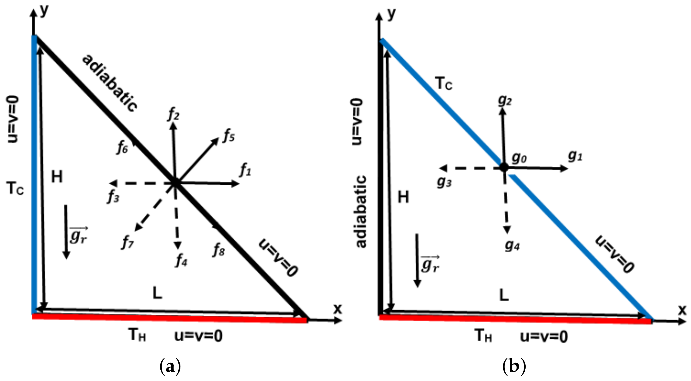
2. Problem Statement

A right-angled triangular and isosceles cavity ($H=L$) enclosing water ($Pr$ = 6.62) was studied numerically using the multirelaxation time lattice Boltzmann method (MRT-LBM). The enclosure considered has a long dimension in the z-direction. Thus, a two-dimensional ($x,y$) cross-section geometry was studied. Natural convection flow was assured by the buoyancy effect, gravity $\left({\mathbf{g}}_r\right)$, and thermal gradient. According to the left and inclined walls thermal boundary conditions, two cases were considered in this study. In the first case, the inclined side of the enclosure was adiabatic, and the horizontal wall was hot, while the left one was kept at a cold temperature (Figure 1a). However, the states of the left and inclined walls were interchanged in the second case (Figure 1b).

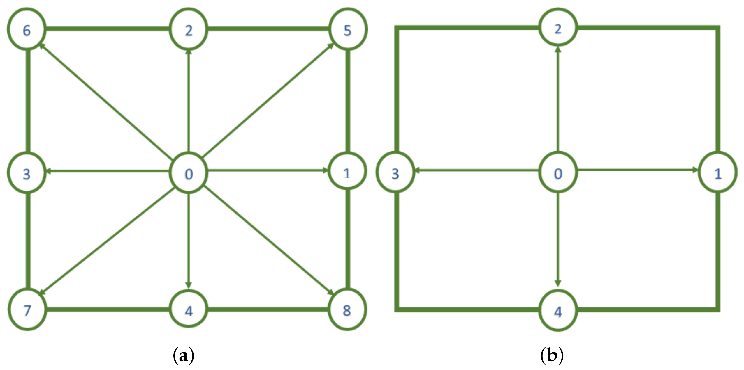
3. Thermal MRT-LBE Model for Fluid Problem

Both fluid flow and thermal behaviors are governed by the Boltzmann equation (BE). According to the MRT-LBM, the distribution functions of flow (f) and temperature (g) fields are governed independently. In the presence of external force per unit of mass ${\mathbf{F}}_k$, the two LB equations are given as

$$f_k\left({\mathbf{x}}_k+{\mathbf{c}}_k\Delta t,t+\Delta t\right)-f_k\left({\mathbf{x}}_k,t\right)={\Omega }_f\left(f_k^{eq}\left({\mathbf{x}}_k,t\right)-f_k\left({\mathbf{x}}_k,t\right)\right)+\Delta t{\mathbf{F}}_k,k=0-8$$

(1)

$$g_k\left({\mathbf{x}}_k+{\mathbf{c}}_k\Delta t,t+\Delta t\right)-g_k\left({\mathbf{x}}_k,t\right)={\Omega }_g\left(g_k^{eq}\left({\mathbf{x}}_k,t\right)-g_k\left({\mathbf{x}}_k,t\right)\right),k=0-4.$$

(2)

where ${\Omega }_f$ and ${\Omega }_g$ represent the collision matrices for f and g, respectively; and ${\mathbf{c}}_k$ and $\Delta t$ are, respectively, the lattice velocity vector in the k-direction and the time step.

The Maxwell distribution functions $f_k^{eq}$ and $g_k^{eq}$ were used during the initialization of the macroscopic properties of flow, the velocity $\mathbf{u}$, and the temperature T. Their expressions are written in the Taylor expansion as

$$f_k^{eq}=w_k\rho \left[1+3{\displaystyle \frac{{\mathbf{c}}_k.\mathbf{u}}{c^2}}+{\displaystyle \frac{9}{2}}{\displaystyle \frac{{\left({\mathbf{c}}_k.\mathbf{u}\right)}^2}{c^4}}-{\displaystyle \frac{3}{2}}{\displaystyle \frac{{\mathbf{u}}^2}{c^2}}\right],$$

(3)

$$g_k^{eq}=w_k^{\prime }T\left[1+3{\displaystyle \frac{{\mathbf{c}}_k.\mathbf{u}}{c^2}}\right],$$

(4)

where c is the lattice speed given by $c={\displaystyle \frac{\Delta x}{\Delta t}}={\displaystyle \frac{\Delta y}{\Delta t}}$, $\Delta x$, and $\Delta y$ are the grid spacing in the x and y-directions, respectively.

In this study, the discrete schemes D2Q9 and D2Q5 (Figure 2a,b) were used for the flow and temperature fields, respectively. The weights $w_k$ and lattices velocities ${\mathbf{c}}_k$ for the D2Q9 model are given, respectively, by

$w_0=4/9$, $w_{1-4}=1/9$, and $w_{5-8}=1/36$.

$${\mathbf{c}}_k=\left\{\begin{array}{c}(0,0),k=0\hfill \\ c(cos\left[(k-1){\displaystyle \frac{\mathsf{\pi }}{2}}\right],sin\left[(k-1){\displaystyle \frac{\mathsf{\pi }}{2}}\right],k=1-4\hfill \\ \sqrt{2}c(cos\left[(k-5){\displaystyle \frac{\mathsf{\pi }}{2}}+{\displaystyle \frac{\mathsf{\pi }}{4}}\right],sin\left[(k-5){\displaystyle \frac{\mathsf{\pi }}{2}}+{\displaystyle \frac{\mathsf{\pi }}{4}}\right],k=5-8\hfill \end{array}\right.$$

The weights $w_k^{\prime }$ and lattices velocities for the D2Q5 model are given, respectively, by

$w_0^{\prime }=1/3$ and $w_k^{\prime }=1/6k=1-4$.

$${\mathbf{c}}_k=\left\{\begin{array}{c}(0,0),k=0\hfill \\ c\left(cos[(k-1){\displaystyle \frac{\mathsf{\pi }}{2}}],sin[(k-1){\displaystyle \frac{\mathsf{\pi }}{2}}]\right),k=1-4\hfill \end{array}\right.$$

Figure 2. (a) D2Q9 and (b) D2Q5 velocities.

Figure 2. (a) D2Q9 and (b) D2Q5 velocities.

The buoyancy-driven force ${\mathbf{F}}_k$ is given in the Boussinesq approximation by [26]

$${\mathbf{F}}_k=3w_k{\mathbf{c}}_k\rho {\mathbf{g}}_r\beta (T-T_{ref}),$$

(5)

where $T_{ref}=(T_H+T_c)/2$, ${\mathbf{g}}_r$, and $\beta$ are the temperature at the reference state, the gravitation vector, and the thermal expansion coefficient, respectively.

In the MRT-LBM model, the streaming process occurs at the microscopic level, in the space formed by the discrete velocities ${\mathbf{c}}_k$, while the collision step takes place in the space of macroscopic moments $(\mathbf{m},\mathbf{n})$, of the distribution functions $(f,g)$. The transition between the two spaces is ensured by the change-over matrices $\mathbf{M}$ for the flow and $\mathbf{N}$ for the temperature, such as

$$\mathbf{m}=\mathbf{M}\mathbf{f} \mathrm{and} \mathbf{f}={\mathbf{M}}^{-\mathbf{1}}\mathbf{m}$$

$$\mathbf{n}=\mathbf{N}\mathbf{g} \mathrm{and} \mathbf{g}={\mathbf{N}}^{-\mathbf{1}}\mathbf{n}$$

where $\mathbf{f}={(f_0,f_1,f_2,f_3,f_4,f_5,f_6,f_7,f_8)}^T$ and $\mathbf{g}={(g_0,g_1,g_2,g_3,g_4)}^T$.

In the SRT model, a single relaxation time is used, while in the MRT model a diagonal relaxation matrix is implemented. The collision operators ${\Omega }_f$ and ${\Omega }_g$ become:

$${\Omega }_f\left(f_k^{eq}\left({\mathbf{x}}_k,t\right)-f_k\left({\mathbf{x}}_k,t\right)\right)={\mathbf{M}}^{-1}{\mathbf{S}}_f\left(m_k^{eq}\left({\mathbf{x}}_k,t\right)-m_k\left({\mathbf{x}}_k,t\right)\right),$$

$${\Omega }_g\left(g_k^{eq}\left({\mathbf{x}}_k,t\right)-g_k\left({\mathbf{x}}_k,t\right)\right)={\mathbf{N}}^{-1}{\mathbf{S}}_g\left(n_k^{eq}\left({\mathbf{x}}_k,t\right)-n_k\left({\mathbf{x}}_k,t\right)\right),$$

where ${\mathbf{S}}_f$ and ${\mathbf{S}}_g$ represent the diagonal relaxation matrices.

The lattice Boltzmann Equations (1) and (2) become:

$$f_k\left({\mathbf{x}}_k+{\mathbf{c}}_k\Delta t,t+\Delta t\right)-f_k\left({\mathbf{x}}_k,t\right)={\mathbf{M}}^{-1}{\mathbf{S}}_f\left(m_k^{eq}\left({\mathbf{x}}_k,t\right)-m_k\left({\mathbf{x}}_k,t\right)\right)+\Delta t{\mathbf{F}}_k,$$

(6)

$$g_k\left({\mathbf{x}}_k+{\mathbf{c}}_k\Delta t,t+\Delta t\right)-g_k\left({\mathbf{x}}_k,t\right)={\mathbf{N}}^{-1}{\mathbf{S}}_g\left(n_k^{eq}\left({\mathbf{x}}_k,t\right)-n_k\left({\mathbf{x}}_k,t\right)\right).$$

(7)

In the k-direction, the parameters $m_k$ and $n_k$ are the moments corresponding to the distribution functions $f_k$ and $g_k$, respectively.

The matrices $\mathbf{M}$ and $\mathbf{N}$ are defined by [10,27]:

$$\mathbf{M}=\left(\begin{array}{ccccccccc}\hfill 1& \hfill 1& \hfill 1& \hfill 1& \hfill 1& \hfill \phantom{-}1& \hfill 1& \hfill 1& \hfill 1\\ \hfill -4& \hfill -1& \hfill -1& \hfill -1& \hfill -1& \hfill 2& \hfill 2& \hfill 2& \hfill 2\\ \hfill 4& \hfill -2& \hfill -2& \hfill -2& \hfill -2& \hfill 1& \hfill 1& \hfill 1& \hfill 1\\ \hfill 0& \hfill 1& \hfill 0& \hfill -1& \hfill 0& \hfill 1& \hfill -1& \hfill -1& \hfill 1\\ \hfill 0& \hfill -2& \hfill 0& \hfill 2& \hfill 0& \hfill 1& \hfill -1& \hfill -1& \hfill 1\\ \hfill 0& \hfill 0& \hfill 1& \hfill 0& \hfill -1& \hfill 1& \hfill 1& \hfill -1& \hfill -1\\ \hfill 0& \hfill 0& \hfill -2& \hfill 0& \hfill 2& \hfill 1& \hfill 1& \hfill -1& \hfill -1\\ \hfill 0& \hfill 1& \hfill -1& \hfill 1& \hfill -1& \hfill 0& \hfill 0& \hfill 0& \hfill 0\\ \hfill 0& \hfill 0& \hfill 0& \hfill 0& \hfill 0& \hfill 1& \hfill -1& \hfill 1& \hfill -1\end{array}\right)$$

$$\mathbf{N}=\left(\begin{array}{ccccc}\hfill 1& \hfill \phantom{-}1& \hfill 1& \hfill 1& \hfill 1\\ \hfill 0& \hfill \phantom{-}1& \hfill 0& \hfill -1& \hfill 0\\ \hfill 0& \hfill \phantom{-}0& \hfill 1& \hfill 0& \hfill -1\\ \hfill -4& \hfill \phantom{-}1& \hfill 1& \hfill 1& \hfill 1\\ \hfill 0& \hfill \phantom{-}1& \hfill -1& \hfill 1& \hfill -1\end{array}\right)$$

The relaxation times of the diagonal matrices $({\mathbf{S}}_f,{\mathbf{S}}_g)$ have a significant influence on the collision phase. For the distribution that one wishes to preserve, a relaxation time equal to unity is allocated. For the nonconservative moments, they undergo a relaxation towards their equilibrium states, defined according to the Bhatnagar–Gross–Krook approximation (BGK) [28] by the following equations:

$${\mathbf{m}}^{\prime }(\mathbf{x},t)=\mathbf{m}(\mathbf{x},t)-{\mathbf{S}}_f\left[\mathbf{m}\left(\mathbf{x},t\right)-{\mathbf{m}}^{eq}\left(\mathbf{x},t\right)\right],$$

(8)

$${\mathbf{n}}^{\prime }(\mathbf{x},t)=\mathbf{n}(\mathbf{x},t)-{\mathbf{S}}_g\left[\mathbf{n}\left(\mathbf{x},t\right)-{\mathbf{n}}^{eq}\left(\mathbf{x},t\right)\right],$$

(9)

where $({\mathbf{m}}^{\prime },{\mathbf{n}}^{\prime })$ are the vectors of moments after the collision, and $({\mathbf{m}}^{eq},{\mathbf{n}}^{eq})$ are their corresponding equilibrium moments vectors.

The diagonal components of the matrices $({\mathbf{S}}_f,{\mathbf{S}}_g)$ are given by:

$${\mathbf{S}}_f=diag\left(\begin{array}{ccccccccc}1& 1.4& 1.4& 1& 1.2& 1& 1.2& s_{f_7}& s_{f_8}\end{array}\right),$$

$${\mathbf{S}}_g=diag\left(\begin{array}{ccccc}1& s_{g_1}& s_{g_2}& 1& 1\end{array}\right),$$

where $s_{f_7}=s_{f_8}=1/{\tau }_f$ and $s_{g_1}=s_{g_2}=1/{\tau }_g$. Note that by taking ($s_{f_k}=1/{\tau }_f$, $k=0-8$) and ($s_{g_k}=1/{\tau }_g$, $k=0-4$), the MRT model is reduced to the SRT one.

The relaxation times ${\tau }_f$ and ${\tau }_g$ are related, respectively, to the kinematic viscosity $\nu$ and thermal diffusivity $\alpha$ by ${\tau }_f=3\nu +0.5$ and ${\tau }_g=\left({\displaystyle \frac{10\alpha }{4+a}}+0.5\right)$. The parameters $\nu$ and $\alpha$ are related to the Prandtl number by the relation: $Pr=\nu /\alpha$.

The parameter a can be freely adjusted to increase the stability of the thermal model by changing the velocity of sound $c_s$. The value $a=-2$ is commonly adopted for this parameter for the D2Q5 model.

At the equilibrium state, the moment vectors $({\mathbf{m}}^{\mathbf{eq}},{\mathbf{n}}^{\mathbf{eq}})$ are given by [10,27]:

$${\mathbf{m}}^{\mathbf{eq}}=\left\{\begin{array}{c}{m}_0^{eq}=\rho \hfill \\ m_1^{eq}=e=-2\rho +3(j_x^2+j_y^2)\hfill \\ m_2^{eq}=\epsilon =\rho -3(j_x^2+j_y^2)\hfill \\ m_3^{eq}=\rho u=j_x\hfill \\ m_4^{eq}=q_x=-j_x\hfill \\ m_5^{eq}=\rho v=j_y\hfill \\ m_6^{eq}=q_y=-j_y\hfill \\ m_7^{eq}=p_{xx}=j_x^2-j_y^2\hfill \\ m_8^{eq}=p_{xy}=j_x{j}_y\hfill \end{array}\right.$$

(10)

$${\mathbf{n}}^{\mathbf{eq}}=\left\{\begin{array}{c}{n}_0^{eq}=T\hfill \\ n_1^{eq}=uT\hfill \\ n_2^{eq}=vT\hfill \\ n_3^{eq}=aT\hfill \\ n_4^{eq}=0\hfill \end{array}\right.$$

(11)

where e is the kinetic energy, $\epsilon =e^2$, $\mathbf{q}(q_x,q_y)$ is the vector of heat flux, $\mathbf{j}(j_x,j_y)$ is the momentum of density, and $(p_{xx},p_{xy})$ are the stress tensor components.

In the following section, normalized variables are used:

$$\theta ={\displaystyle \frac{T-T_c}{T_H-T_c}};(X,Y)=(x,y)/H;(U,V)=(u,v)/V_s,$$

where scale velocity $V_s$ is defined by: $V_s=\sqrt{g\beta (T_H-T_c)H}$. Therefore, the hot and cold temperatures and that of reference state become, respectively, ${\theta }_H=1$, ${\theta }_c=0$, and ${\theta }_{ref}=0.5$.

By fixing Rayleigh number $\left(Ra\right)$, Prandtl number $\left(Pr\right)$, and Mach number $\left(Ma\right)$, the viscosity is calculated by

$$\nu =HMa{c}_s\sqrt{{\displaystyle \frac{Pr}{Ra}}},$$

(12)

where H is the number of lattices in y-direction and Rayleigh number is defined as $Ra={\displaystyle \frac{g\beta H^3({\theta }_H-{\theta }_c)}{\nu \alpha }}$.

To satisfy the incompressibility condition of flow, the Mach number value should be less than 0.3. We set $Ma=0.1$ in this study.

The Nusselt number is one of the most important dimensionless parameters in the description of convective heat transport. The local Nusselt number $N{u}_x$ and its average value $〈Nu〉$ along the hot wall are calculated as follows:

$$N{u}_x={\displaystyle \frac{H}{({\theta }_H-{\theta }_c)}}{\displaystyle \frac{\partial \theta }{\partial y}}{|}_{y=0},$$

(13)

$$〈Nu〉={\displaystyle \frac{1}{H}}{\int }_0^{H}N{u}_{x}dx.$$

(14)

The macroscopic properties of flow, density $\rho$, velocity $\mathbf{u}$, and temperature T are calculated as

$$\rho =\sum _{k=0}^8{f}_k,$$

(15)

$$\mathbf{u}={\displaystyle \frac{1}{\rho }}\sum _{k=0}^8{f}_k{\mathbf{c}}_k,$$

(16)

$$T=\sum _{k=0}^4{g}_k.$$

(17)

In this study, the three walls are considered at rest with no-slip boundary condition ($u=v=0$). At the inclined wall, the unknown distribution functions (dashed lines) $f_{k=3/4/7}$ (see Figure 1a) can be determined from the known ones $f_{k=1/2/5}$ by

$$f_3=f_1,$$

(18)

$$f_4=f_2,$$

(19)

$$f_7=f_5.$$

(20)

At the adiabatic wall, the bounce-back boundary condition is also used. The temperature at the isothermal walls is known (hot and cold walls). Because we use D2Q5, the unknown internal energy distribution functions are evaluated, respectively, as follows:

• At the inclined adiabatic wall (case 1), the unknown distribution functions $g_{k=3/4}$ can be determined from the known ones $g_{k=1/2}$ by:

$$g_3=g_1,$$

(21)

$$g_4=g_2.$$

(22)

• At the horizontal hot wall (case 1 and 2), the unknown distribution function $g_2$ can be determined from the known ones $g_{k=0/1/3/4}$ by:

$$g_2={\theta }_H-g_0-g_1-g_3-g_4.$$

(23)

• At the inclined cold wall (case 2), the unknown distribution functions $g_{k=3/4}$ (see Figure 1b) can be determined from the known ones $g_{k=0/1/2}$ by:

$$g_3=g_4=0.5({\theta }_c-g_0-g_1-g_2).$$

(24)

4. Results and Discussion

A FORTRAN code was adopted to simulate numerically water natural convection flow within a triangular cavity. Two cases were considered in this study, according to the left and inclined walls thermal boundary conditions (Figure 1a,b). The first case was carried out experimentally and numerically (FLUENT) by Yesiloz et al. [16] and also by Mejri et al. [19] using SRT-LBM. However, in this study, the MRT-LBM model was adopted.

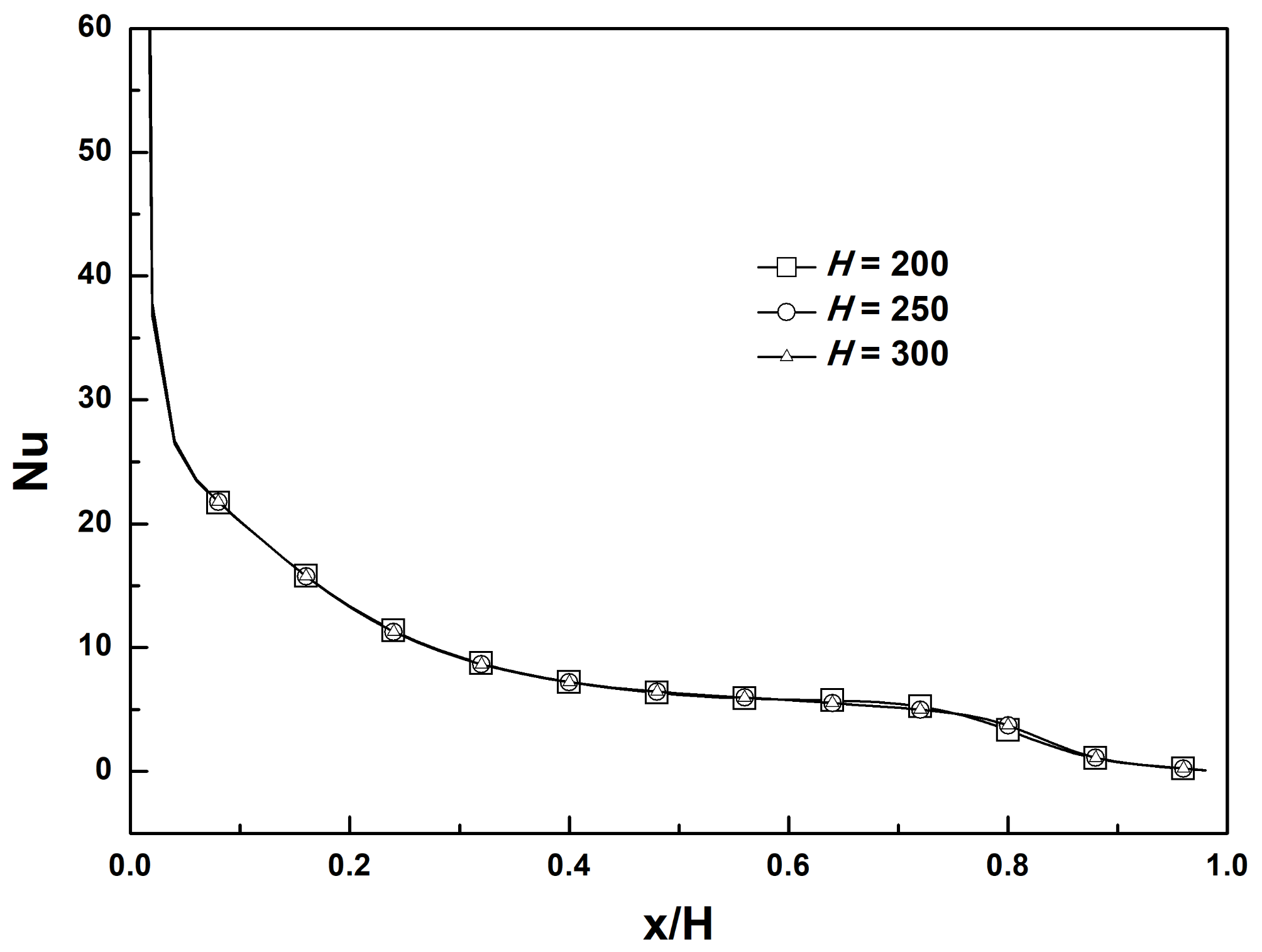
4.1. Mesh Independence Study

To test the grid size effect on the results, the profiles of Nusselt number along the heated wall (first case) for different values of the characteristic length of the cavity (H) were plotted for $Ra={10}^6$ (Figure 3).

Table 1. Effect of the length H on the value of ${\psi }_{max}$ and $\theta (1/3,2/3)$ for $Ra={10}^6$-case 1.

H	150	200	250	300
${\psi }_{max}$	32.67627	32.79659	32.65666	32.14074
$\theta (1/3,2/3)$	0.64222	0.64456	0.64215	0.64171

shows the maximum value of the streamlines $\left({\psi }_{max}\right)$ and the temperature on the adiabatic wall at $(1/3,2/3)$ for different values of H. By analyzing the results, the length of $H=250$ was enough to give good results and was adopted for all the following simulations.

Note that the minimum value of the stream function $\left({\psi }_{min}\right)$ in the first case and its maximum value $\left({\psi }_{max}\right)$ in the second case are equal to zero for all $Ra$ tested values in this work.

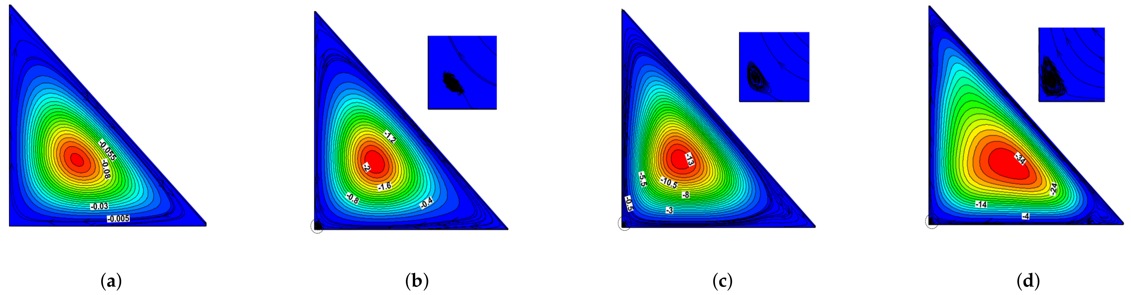
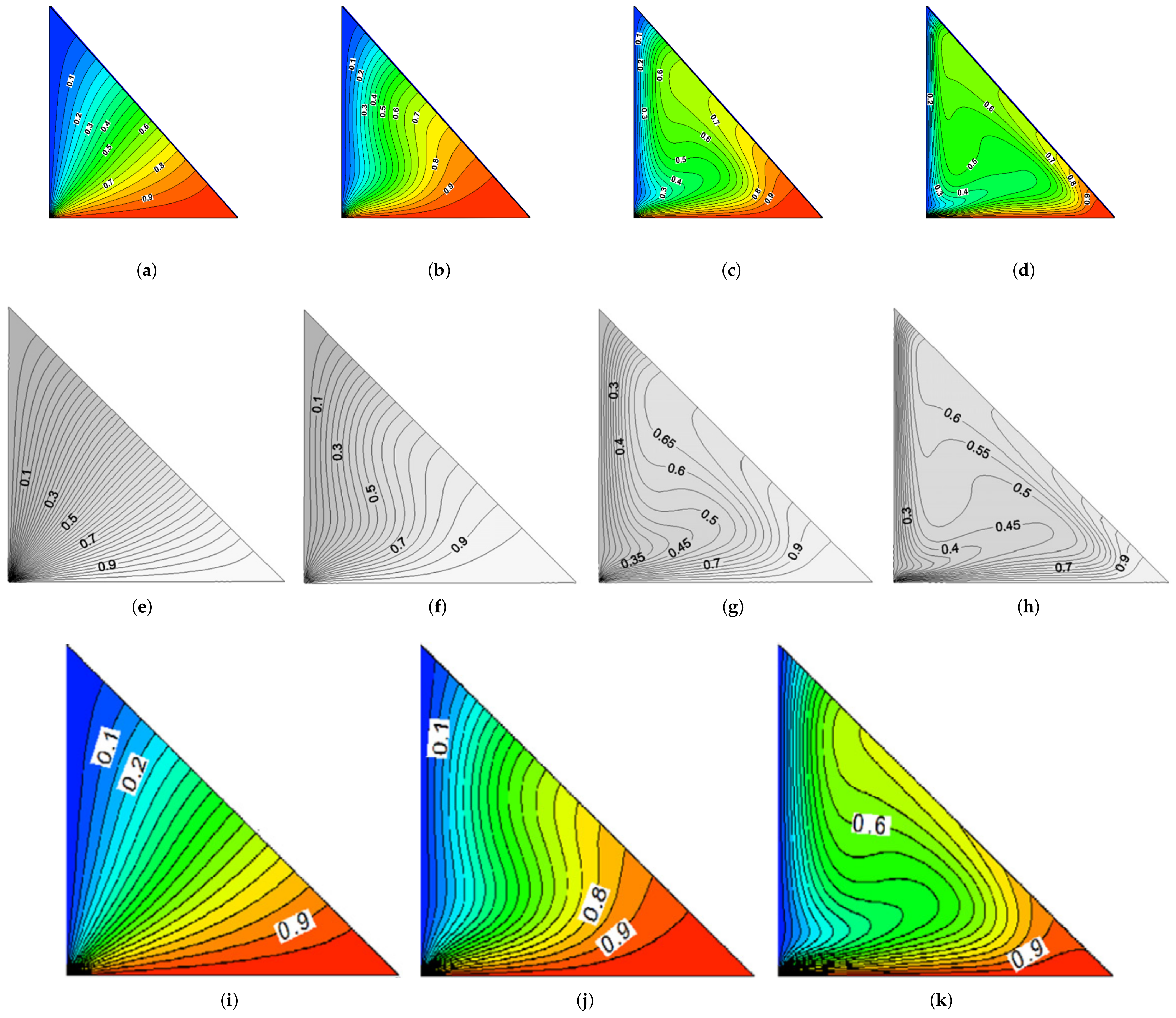
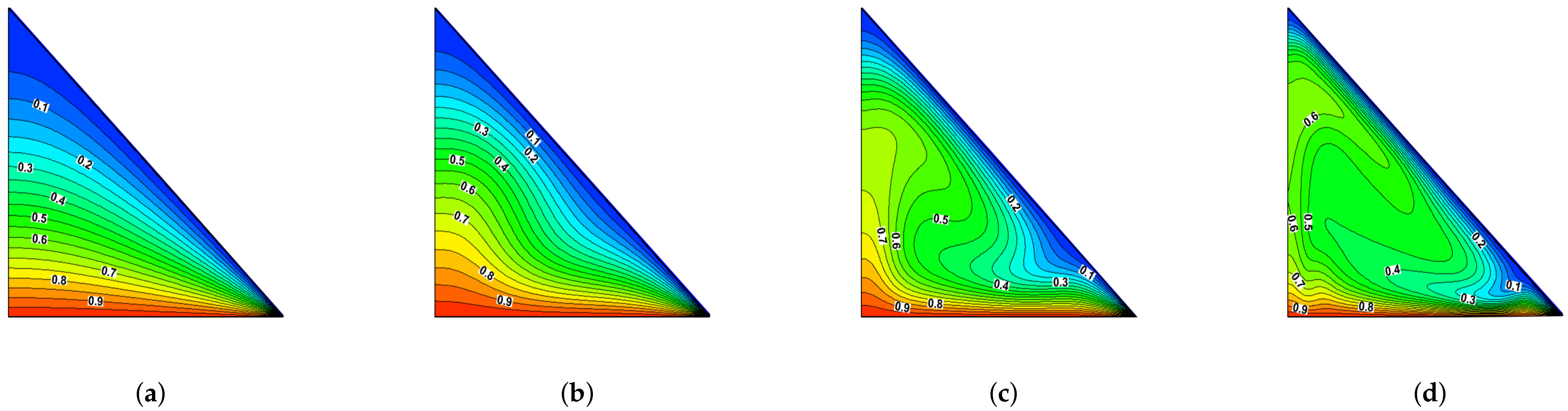
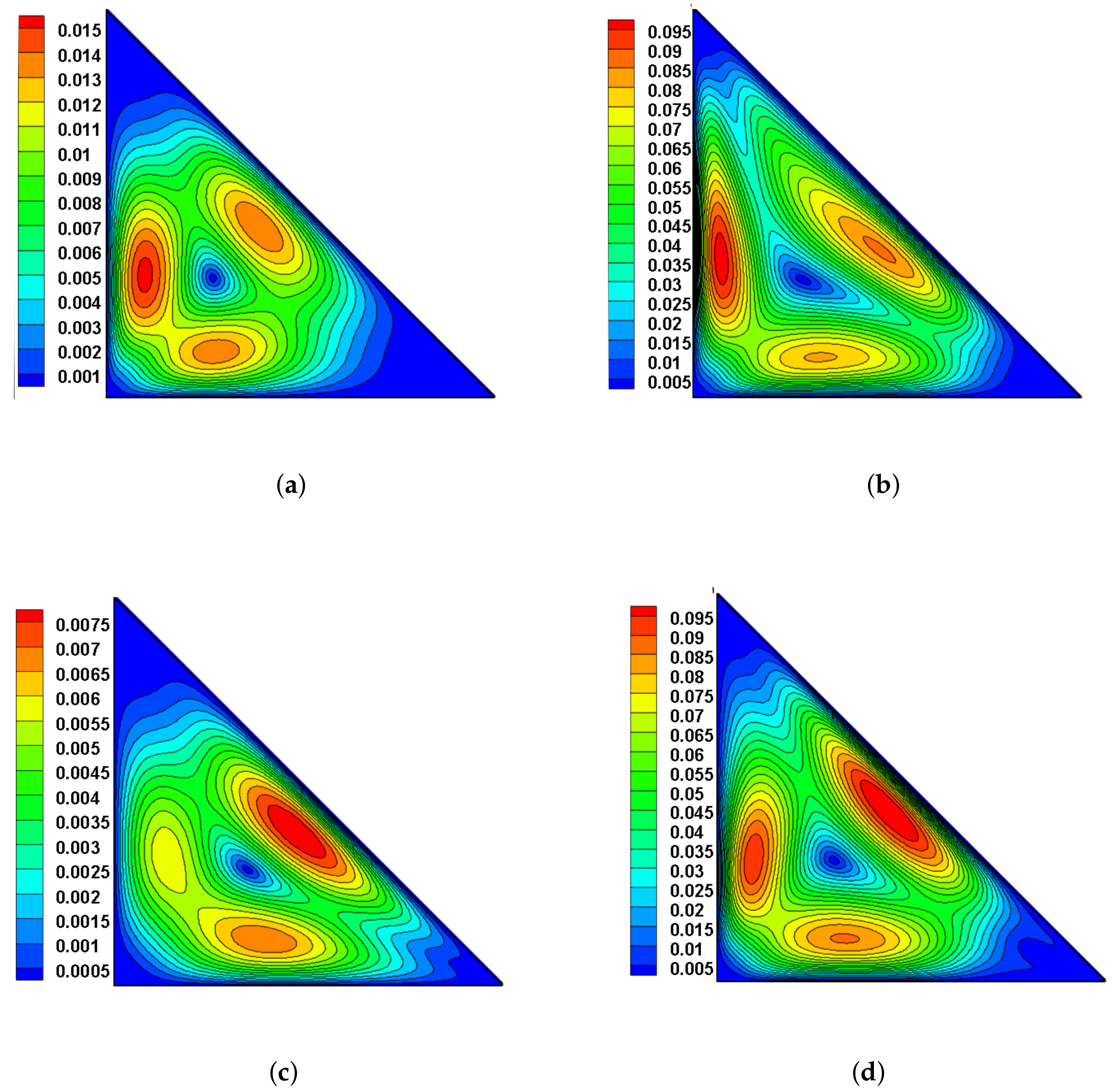
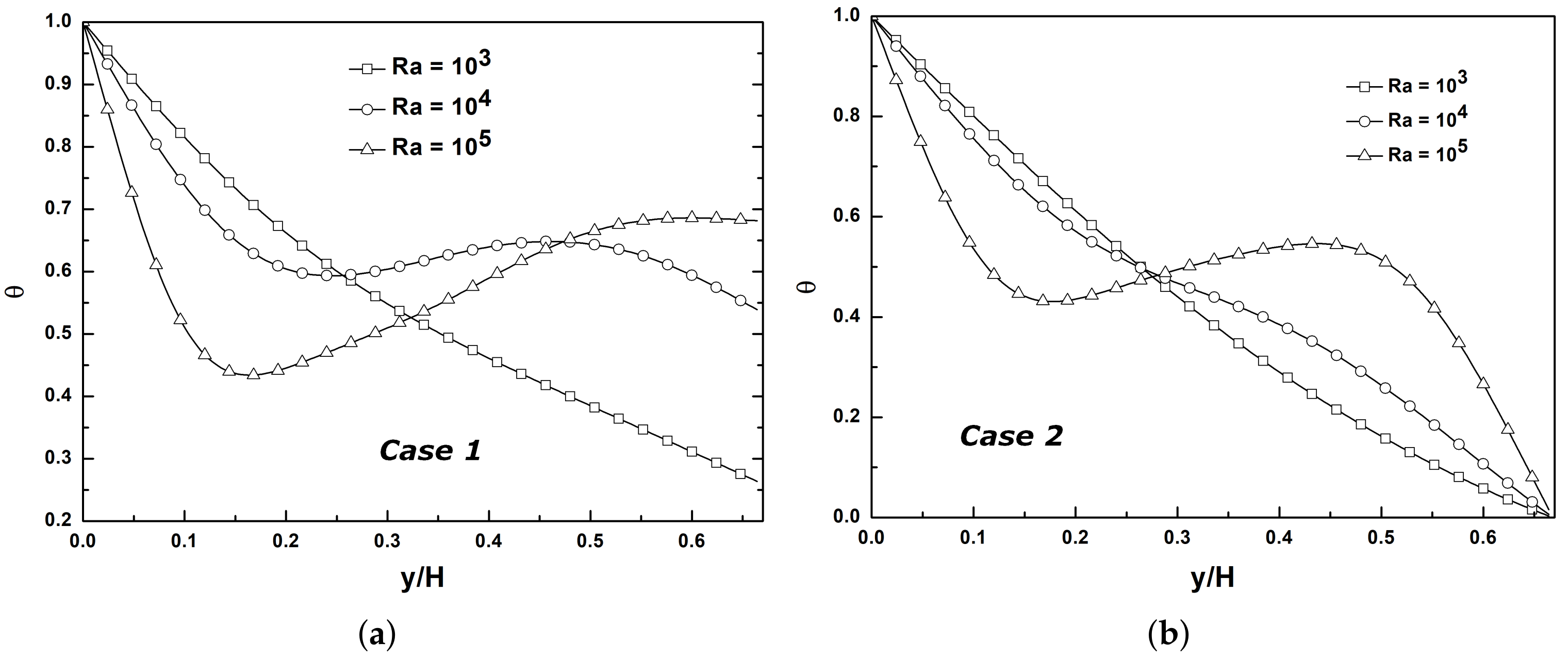
4.2. Validation and Discussion of Flow Properties

Figure 4, Figure 5, Figure 6 and Figure 7 illustrate the effect of the Rayleigh number, on the streamlines and the isotherms, respectively, for first and second cases. For low Rayleigh number $(Ra={10}^3)$, the conduction regime is dominant, and weak circulation of flow in the cavity is found (${\psi }_{max}\approx 0.216$ for case 1 and ${\psi }_{min}\approx -0.105$ for case 2). The flow intensity increases with Rayleigh number, as expected, and it is clearly seen through the examination of the maximum and minimum stream function values given in

Table 2. Values of ${\psi }_{max}$ for case 1 and ${\psi }_{min}$ for case 2 for different $Ra$.

	$\mathbf{Ra}$	${10}^3$	${10}^4$	${10}^5$	$5\times {10}^5$
${\psi }_{max}$-case 1	Present study	0.216	2.62	12.09	25.47
	Yesiloz  et al. [16]	0.215	2.62	12.12	25.51
	Mejri et al. [19]	0.23	2.57	11.70	$---$
${\psi }_{min}$-case 2	Present study	−0.105	−2.08	−13.35	−27.48

. For values of Rayleigh number above ${10}^5$, convection is more pronounced. The maximum value of the stream function, for the Rayleigh number equal to $5\times {10}^5$, is almost 117 times larger than its value when the Rayleigh number is equal to ${10}^3$ for the first case. However, in the second case, the minimum value of the stream function decreases almost 261 times (negative values) for the same values of $Ra$, which proves that convection is more dominant in the second case (Table 2). A large vortex (primary) is formed inside the cavity in the clockwise rotation in the second case, while it is in the counter-clockwise direction in the first case. The particles close to the hot wall move rapidly upwards and their place is therefore filled by the slower colder particles; they lose a part of their thermal energy, and their temperature decreases, which pushes them to join a warmer region. In both cases, the particles during their movement follow HAC (Hot-Adiabatic-Cold) circulation. The increase in the Rayleigh number increases the intensity of these vortices and decreases the boundary layer thickness near the hot wall, indicating the presence of an intense temperature gradient, therefore giving a strong heat transfer rate in this region. For $Ra={10}^3$, streamlines produce a primary vortex located near the gravity center of the cavity. As the Rayleigh number increases ($Ra={10}^4$ and ${10}^5$), the streamlines structure is still generally unaffected, except the center of the primary vortex, which takes an elliptical shape for both cases. It should be noted that the stream function intensity is very low, and flow cannot penetrate in all the corner zones. By increasing the value of $Ra$ the flow enlarges from the bulk to the walls, and this leads to the propagation of the flow toward the narrow corner regions. In the first case, for values of ${10}^3\le Ra\le {10}^5$, the primary vortex undergoes a slight movement from left to right by increasing the value of $Ra$. The great convection forces this vortex to undergo a displacement in the opposite direction for $Ra={10}^6$ which shows that the flow is close to the turbulent regime. (

Table 3. Position of the primary vortex $(x/H,y/H)$ for different $Ra$.

$\mathbf{Ra}$	${10}^3$	${10}^4$	${10}^5$	$5\times {10}^5$
Case 1	(0.275, 0.31)	(0.278, 0.31)	(0.283, 0.30)	(0.260, 0.31)
Case 2	(0.343, 0.299)	(0.310, 0.309)	(0.302, 0.312)	(0.292, 0.323)

) presents primary vortices center changes with the increase in Rayleigh number. In the first case, changes are observed only in the positive x-direction, while its direction in the second case is slightly directed to the upper-left corner. In the two cases, by increasing Ra, the primary vortex center is directed toward the adiabatic plate. The secondary vortex is located in the corner between the cold and adiabatic walls, this vortex narrows, and progressively, its center undergoes a movement from bottom to top by increasing the value of $Ra$ (Figure 4a–d). In the second case (Figure 5), by increasing the value of $Ra$, the primary vortex undergoes a slight displacement from right to left and from bottom to top. This vortex keeps the same displacement along x and y directions, even for the value of ${10}^6$. The secondary vortex appears for $Ra\ge {10}^4$, it is located in the corner between the hot and adiabatic walls, and its volume becomes more meager gradually until it almost vanishes near the two walls for $Ra{10}^6$ (Figure 5b–d). The MRT-LBM method predicts the position of the secondary vortices for weak stream function ($\psi$ close to 0). For both cases, it can be seen that the heat transfer is mainly governed by conduction in the corners of the cavity for the values of the Rayleigh number ranging from ${10}^3$ to ${10}^6$. The flow cannot reach all the corners and inactive hydrodynamic regions, and it appears from the absence of vortices in these regions.

Figure 6 and Figure 7 show isotherms obtained from the numerical simulations and experimental results. For $Ra={10}^3$, the isotherms exhibit the characteristics of pure conduction forming a diagonally antisymmetric structure with respect to $\theta =0.5$ in the first case since the intensity of the buoyancy-driven convection is very weak, and then the thermal field is thus unaffected. However, in the second case, this antisymmetry is not as in the first one perfect. The isotherm profiles show that the dominance of the convection on transport increases in the enclosure by increasing the Rayleigh number for both cases. For the higher values of $Ra$, isotherms become more constricted near the hot and cold walls. However, these isotherms near and on the adiabatic wall always remain expanded. Convection is dominant for high Rayleigh numbers, which causes the reduction of the boundary layer. This decrease in the boundary layer can also be seen by the distribution of isotherms.

The heat-transfer characteristics of the flow are determined using the dimensionless Nusselt number $Nu$. It characterizes the heat-transfer mode involved, whether convective or conductive heat transfer or both of them. As the Rayleigh number increases, the average Nusselt number $〈Nu〉$ calculated along the bottom wall undergoes an increase in both cases. Note that for the same value of $Ra$, the value of $〈Nu〉$ in the second case is greater than those of the first case, which means the dominance of the convection in case 2 (

Table 4. Average Nusselt number $〈Nu〉$ for different $Ra$.

$\mathbf{Ra}$	${10}^3$	${10}^4$	${10}^5$	$5\times {10}^5$
Case 1	4.60	4.88	6.83	8.03
Case 2	7.61	7.77	9.74	11.94

).

Figure 8a–d show the profiles, respectively, of u-velocity along the vertical line $x/H=1/3$ and of v-velocity along the horizontal line $y/H=1/3$ for $Ra={10}^3-{10}^5$. According to these figures, the maximum magnitude of horizontal and vertical velocities increases significantly with the increase in the Rayleigh number. For $y/H<0.33$, the values of the horizontal component of the velocity are positive for the first case, while they are negative for the second case. An alternation of these observations is shown for the vertical component of the velocity. This confirms the direction of the vortex observed. Convection becomes dominating as the magnitudes of velocity components increase, confirming what was previously mentioned. Note that at the walls, the two components of the velocity are equal to zero, since the bounce-back boundary condition is applied. In both cases, the larger values of the velocity magnitude are found near the cold wall. Almost zero values are observed near the triangle cavity’s corners as well as its center. By increasing the value of $Ra$, the values of $\left|\right|\mathbf{u}\left|\right|$ increase and undergo diffusion progressive to the corners. The values of $\left|\right|\mathbf{u}\left|\right|$ increase almost 6 times in the first case, while in the second case they undergo an increase of almost 12 times as $Ra$ passes from ${10}^3$ to ${10}^5$. This observation shows the great effect of hot and cold walls positions on this magnitude and also on the convection process (Figure 9a–d).

The temperatures of hot and cold walls are unchanged, while the adiabatic wall interacts and undergoes a variation of temperature during free convection. Figure 10a,b show the dimensionless temperature profiles along the y-axis for $x/H=1/3$ and Rayleigh numbers $Ra={10}^3-{10}^5$. In the first case, for $Ra={10}^3$, the conduction mode is dominant, and the temperature undergoes a gradual decrease along this axis. Note that the low-temperature variation (profile horizontal) along the y-axis for $Ra={10}^4-{10}^5$ indicates the existence of a homogeneous temperature. As the Rayleigh number increases, the temperature increases at the point $(1/3,2/3)$ on the adiabatic wall under the effect of the convection. In the second case, the temperature varies from ${\theta }_H$ to ${\theta }_c$ along this axis. For the values $Ra={10}^3$ and ${10}^4$, the temperature undergoes a progressive variation, while for $Ra={10}^5$, the almost horizontal profile indicates the existence of a homogeneous temperature following large convection.

To sum up, by using the method MRT-LBM, the results obtained are closer to those of Yesiloz et al. [16] than those obtained by the SRT-LBM [19]. This method predicts the position of the secondary vortices even for weak stream function for both cases. The position of cold and adiabatic walls in enclosed right-angled triangular and isosceles cavity has a great influence on the results of streamlines, isotherms, and average Nusselt number, and the convection is more dominant in the second case.

5. Conclusions

According to the left and inclined walls thermal boundary conditions, two cases were studied of incompressible flow confined within a right-angled triangular and isosceles cavity. In the first case, the inclined side of the enclosure was adiabatic, while the left one was kept at a cold temperature. However, the temperature states of the left and inclined walls were reversed in the second case. The range of the Rayleigh number discussed is from ${10}^3$ to ${10}^6$. The effect of the Rayleigh number on streamlines, isotherms, and average Nusselt number was studied. The maximum and minimum values of the stream function (${\psi }_{max}$ in case 1 and $|{\psi }_{min}|$ in case 2), heat-transfer rate (isotherms), and average Nusselt number increase with the growth of Rayleigh number. Isotherms become more constricted near the hot and cold walls for the great values of $Ra$ number. Good agreement can be observed between the present simulation results and the literature previously published. Finally, in this research, the efficiency of the MRT-LBM to simulate natural convection is demonstrated and shows its capability to treat such problems.

References

1. Shan, X. Simulation of Rayleigh-Bénard convection using a lattice Boltzmann method. Phys. Rev. E 1997, 55, 2780. [Google Scholar] [CrossRef] [Green Version]
2. Sarris, I.E.; Lekakis, I.; Vlachos, N.S. Natural convection in a 2D enclosure with sinusoidal upper wall temperature. Numer. Heat Transf. Part A Appl. 2002, 42, 513–530. [Google Scholar] [CrossRef]
3. Tric, E.; Labrosse, G.; Betrouni, M. A first incursion into the 3D structure of natural convection of air in a differentially heated cubic cavity, from accurate numerical solutions. Int. J. Heat Mass Transf. 2000, 43, 4043–4056. [Google Scholar] [CrossRef]
4. Peng, Y.; Shu, C.; Chew, Y.T. A 3D incompressible thermal lattice Boltzmann model and its application to simulate natural convection in a cubic cavity. J. Comput. Phys. 2004, 193, 260–274. [Google Scholar] [CrossRef]
5. Akinsete, V.A.; Coleman, T.A. Heat transfer by steady laminar free convection in triangular enclosures. Int. J. Heat Mass Transf. 1982, 25, 991–998. [Google Scholar] [CrossRef]
6. Asan, H.; Namli, L. Numerical simulation of buoyant flow in a roof of triangular cross-section under winter day boundary conditions. Energy Build. 2001, 33, 753–757. [Google Scholar] [CrossRef]
7. Bejan, A. Convection Heat Transfer; John Wiley & Sons: Hoboken, NJ, USA, 2013. [Google Scholar]
8. Yang, K.T. Natural convection in enclosures. In Handbook of Single-Phase Convective Heat Transfer; Taylor & Francis: Abingdon, UK, 1987. [Google Scholar]
9. Hasnaoui, M.; Mansouri, A.E.; Amahmid, A. MRT-LBM simulation of natural convection in a Rayleigh-Benard cavity with linearly varying temperatures on the sides: Application to a micropolar fluid. Front. Heat Mass Transf. 2017, 9. [Google Scholar] [CrossRef] [Green Version]
10. Mezrhab, A.; Moussaoui, M.A.; Jami, M. Double MRT thermal lattice Boltzmann method for simulating convective flows. Phys. Lett. A 2010, 374, 3499–3507. [Google Scholar] [CrossRef]
11. Hssikou, M.; Elguennouni, Y.; Baliti, J.; Alaoui, M. Heat Transfer of Gas Flow within a Partially Heated or Cooled Square Cavity. Model. Simul. Eng. 2020, 2020, 8886682. [Google Scholar] [CrossRef]
12. Hssikou, M.; Elguennouni, Y.; Baliti, J.; Alaoui, M. Lattice Boltzmann method for natural convection in a square cavity with a heated chip. In Proceedings of the International Conference on Intelligent Systems and Advanced Computing Sciences (ISACS), Taza, Morocco, 26–27 December 2019; pp. 1–7. [Google Scholar]
13. Basak, T.; Roy, S.; Babu, S.K.; Balakrishnan, A.R. Finite element analysis of natural convection flow in a isosceles triangular enclosure due to uniform and non-uniform heating at the side walls. Int. J. Heat Mass Transf. 2008, 51, 4496–4505. [Google Scholar] [CrossRef]
14. Kent, E.F. Numerical analysis of laminar natural convection in isosceles triangular enclosures. Proc. Inst. Mech. Eng. Part D J. Mech. Eng. Sci. 2009, 223, 1157–1169. [Google Scholar] [CrossRef]
15. Saleem, K.B.; Alshara, A.K. Natural convection in a triangular cavity filled with air under the effect of external air stream cooling. Heat Transf. Res. 2019, 48, 3186–3213. [Google Scholar] [CrossRef]
16. Yesiloz, G.; Orhan, A. Laminar natural convection in right-angled triangular enclosures heated and cooled on adjacent walls. Int. J. Heat Mass Transf. 2013, 60, 365–374. [Google Scholar] [CrossRef]
17. Oztop, H.F.; Varol, Y.; Koca, A.; Firat, M. Experimental and numerical analysis of buoyancy-induced flow in inclined triangular enclosures. Int. Commun. Heat Mass Transf. 2012, 39, 1237–1244. [Google Scholar] [CrossRef]
18. Mahmoudi, A.; Mejri, I.; Ammar, M.A.; Omri, A. Numerical study of natural convection in an inclined triangular cavity for different thermal boundary conditions: Application of the lattice Boltzmann method. Fluid Dyn. Mater. Process 2013, 9, 353–388. [Google Scholar]
19. Mejri, I.; Mahmoudi, A.; Abbassi, M.A.; Omri, A. LBM Simulation of natural convection in an inclined triangular cavity filled with water. Alex. Eng. J. 2016, 55, 1385–1394. [Google Scholar] [CrossRef] [Green Version]
20. Ridouane, E.H.; Campo, A.; Hasnaoui, M. Turbulent natural convection in an air-filled isosceles triangular enclosure. Int. J. Heat Fluid Flow 2006, 27, 476–489. [Google Scholar] [CrossRef]
21. Koca, A.; Oztop, H.F.; Varol, Y. The effects of Prandtl number on natural convection in triangular enclosures with localized heating from below. Int. Commun. Heat Mass Transf. 2007, 34, 511–519. [Google Scholar] [CrossRef]
22. Shahid, H.; Yaqoob, I.; Khan, W.A.; Rafique, A. Mixed convection in an isosceles right triangular lid driven cavity using multi relaxation time lattice Boltzmann method. Int. Commun. Heat Mass Transf. 2021, 128, 105552. [Google Scholar] [CrossRef]
23. Rahmati, A.R.; Niazi, S. Application and comparison of different lattice Boltzmann methods on non-uniform meshes for simulation of micro cavity and micro channel flow. Comput. Methods Eng. 2015, 34, 97–118. [Google Scholar] [CrossRef] [Green Version]
24. Elguennouni, Y.; Hssikou, M.; Baliti, J.; Alaoui, M. Numerical study of gas microflow within a triangular lid-driven cavity. Adv. Sci. Technol. Eng. Syst. J. 2020, 5, 578–591. [Google Scholar] [CrossRef]
25. Mallinson, G.D.; Davis, G.D.V. Three-dimensional natural convection in a box: A numerical study. J. Fluid Mech. 1977, 83, 1–31. [Google Scholar] [CrossRef]
26. Mohammed, A.A. Lattice Boltzmann Method: Fundamentals and Engineering Applications with Computer Codes; Springer Nature: London, UK, 2019. [Google Scholar]
27. Mezrhab, A.; Jami, M.; Bouzidi, M.; Lallemand, P. Analysis of radiation–natural convection in a divided enclosure using the lattice boltzmann method. Comput. Fluids 2007, 36, 423–434. [Google Scholar] [CrossRef]
28. Bhatnagar, P.L.; Gross, E.P.; Krook, M. A model for collision processes in gases. I. Small amplitude processes in charged and neutral one-component systems. Phys. Rev. 1954, 94, 511–525. [Google Scholar] [CrossRef]
Figure 1. Studied configurations: (a) case 1 and (b) case 2.
Fluids 07 00074 g001
Figure 3. Profiles of Nusselt number along the heated wall for different H values-case 1.
Fluids 07 00074 g003
Figure 4. Streamlines-case 1 (ad) Present study for R a = 10 3 , 10 4 , 10 5 , and 10 6 ; (eh) numerical results of Yesiloz et al. [16] for R a = 10 3 , 10 4 , 10 5 , and 10 6 ; (i,j) experimental results of Yesiloz et al. [16] for R a = 10 5 and 10 6 ; and (km) numerical results of Mejri et al. [19] for R a = 10 3 , 10 4 , and 10 5 . Plots (ej) reproduced with permission from [16], published by Elsevier 2013; plots (km) reproduced from [19], published by Elsevier 2016.
Fluids 07 00074 g004
Figure 5. Streamlines of present study-case 2 (ad) for R a = 10 3 , 10 4 , 10 5 , and 10 6 .
Fluids 07 00074 g005
Figure 6. Isotherms-case 1 (ad) Present study for R a = 10 3 , 10 4 , 10 5 , and 10 6 ; (eh) numerical results of Yesiloz et al. [16] for R a = 10 3 , 10 4 , 10 5 , and 10 6 (reproduced with permission from [16], published by Elsevier 2013); and (ik) numerical results of Mejri et al. [19] for R a = 10 3 , 10 4 , and 10 5 (reproduced from [19], published by Elsevier 2016).
Fluids 07 00074 g006
Figure 7. Isotherms of present study-case 2 (ad) for R a = 10 3 , 10 4 , 10 5 , and 10 6 .
Fluids 07 00074 g007
Figure 8. (a,b) Profiles of u-velocity along the line x / H = 1 / 3 and (c,d) profiles of v-velocity along the line y / H = 1 / 3 for R a = 10 3 10 5 -case 1 and 2.
Fluids 07 00074 g008
Figure 9. Contours of velocity modulus (a,b) for R a = 10 3 and R a = 10 5 -case 1 and (c,d) for R a = 10 3 and R a = 10 5 -case 2.
Fluids 07 00074 g009
Figure 10. Profiles of temperature along the vertical line passing by x / H = 1 / 3 for R a = 10 3 10 5 (a) case 1 and (b) case 2.
Fluids 07 00074 g010