Abstract
This paper presents a new nonlinear projection based model reduction using convolutional Variational AutoEncoders (VAEs). This framework is applied on transient incompressible flows. The accuracy is obtained thanks to the expression of the velocity and pressure fields in a nonlinear manifold maximising the likelihood on pre-computed data in the offline stage. A confidence interval is obtained for each time instant thanks to the definition of the reduced dynamic coefficients as independent random variables for which the posterior probability given the offline data is known. The parameters of the nonlinear manifold are optimized as the ones of the decoder layers of an autoencoder. The parameters of the conditional posterior probability of the reduced coefficients are the ones of the encoder layers of the same autoencoder. The optimization of both sets of the encoder and the decoder parameters is obtained thanks to the application of a variational Bayesian method, leading to variational autoencoders. This Reduced Order Model (ROM) is not a regression model over the offline pre-computed data. The numerical resolution of the ROM is based on the Chorin projection method. We apply this new nonlinear projection-based Reduced Order Modeling (ROM) for a 2D Karman Vortex street flow and a 3D incompressible and unsteady flow in an aeronautical injection system.
1. Introduction
Incompressible and transient flows in aeronautics are solved when considering optimal control and parts design. This problem usually needs computational cost reduction in order to perform the optimization with a reasonable computation cost, i.e., with both controlled return time and computational hardware. Hence, we need to construct a reduced model of an unsteady simulation in fluid dynamics. Model reduction is a large scientific field where various approaches have been proposed. We can classify these approaches into two main classes: the physics-based or physics-informed model reduction and the black-box model reduction. In the first class, the equations of physics are used either to solve the reduced model [1,2,3] or to train a machine learning model with a physics-informed cost function which is often given by the residual of the partial differential Equations [4,5,6]. In the second class, the equations of physics are ignored, and a mapping between the inputs and the outputs is learned thanks to linear or nonlinear regression approaches [7,8,9].
In this paper, we are interested in physics-based model reduction. More particularly, we are interested in being capable of reproducing accurately and efficiently transient and incompressible flows. Many research papers in this class of reduction techniques have tried to find a solution to this problem. The answer is far from being completely known, and this field is still an active area of research. POD applied to a transient turbulent flow as a data compression technique [10,11] has proved to be an important tool to reproduce the coherent structures of the flow i.e., the ones which are responsible for the production of the turbulent kinetic energy. In general, a reduced number of POD modes may represent most of the large scales’ turbulent kinetic energy. This linear data compression approach was then widely used to perform a Galerkin projection of the unsteady Navier–Stokes equations upon the reduced vector space spanned by a reduced number of POD modes. However, when injecting the POD modes in the momentum conservation equations, a stability issue may rise even if the POD modes contain the velocity coherent structures and are capable of compressing the unsteady fields well. This stability issue is often remarked for unsteady and turbulent flows, for which the small vortices are required in order to dissipate the large scales kinetic energy and to assure energy conservation; see [12] where a POD basis is obtained with respect to eigenvectors associated with the -temporal correlations matrix [13], where an artificial viscosity is considered within the reduced order model [14], where an enrichment of the classical POD space is obtained with the velocity modes associated with the -temporal correlations matrix and [15], where a reduced order model inspired from the variational multiscale approach is developed. Theoretical studies of a priori error estimates [16] associated with the POD-Galerkin ROM applied to the incompressible and unsteady Navier–Stokes showed that this error is upper bounded and controlled by the remainder of the POD eigenvalues sum if the coercivity constant is larger than the norm of the semi-discretized convective term in the Hilbert space of the squared integrable functions over an open and bounded set. Otherwise, the a priori upper bound of the POD-Galerkin ROM error is expressed as the remainder of the POD eigenvalues sum multiplied by the exponential of the current time instant. In [14], a solution to this problem was addressed by modelling the gradient of the fluctuating velocity field within the reduced order space. A new linear approximation space accounting for the dominant nonlinear behavior was proposed in order to reduce the norm of the semi-discretized convective term.
This stability issue was also formulated in the paper of Grimberg et al. [17] as related to convection dominated problems in general, which might include laminar and turbulent flows. The main argument is the fact that, for these problems, the tangent operators are not symmetric positive definite; therefore, the hypothesis of the orthogonality of the residual of the equations or its Jacobian with respect to the linear POD reduced order space, as it is stated in the Galerkin approach, is no longer valid. This can be seen easily by looking closely into the Newton–Raphson method. A Least Square Petrov–Galerkin (LSPG) approach is proposed instead. Many other authors in the literature also mentioned stability problems in the POD-Galerkin applied to the incompressible Navier–Stokes equations. They related this stability to the modeling of the pressure term in the Galerkin formulation, which is often omitted from this latter by considering the poor effect of the pressure field on the outlet boundary on the velocity field. It has been shown in Noack et al. [18] that, for 2D cases, the surface integral term containing the pressure field has an important impact on the POD-Galerkin ROM result. In Rozza et al. [19], where the impact of the pressure field was also studied for POD-Galerkin approaches, a stabilization approach was proposed inspired from the Chorin projection technique. In the literature, we can find an ensemble of papers that tried to tackle POD-Galerkin instabilities for the Navier–Stokes equations, by adding some numerical least square constraints that enforce the convergence of the reduced order coefficients towards the ones obtained simply by the orthogonal projection of the pre-computed high-fidelity solutions onto a reduced number of their POD modes; see the work of Baiges et al. [20] and Willcox et al [21].
Recently, nonlinear data compression based on neural networks in particular on autoencoders [22] have arisen in the field of the reduced order modeling of parabolic equations. In this case, the approximation of the solutions space is described by a nonlinear manifold that maximizes the likelihood with respect to the pre-computed high-fidelity solutions. We cite the work of Kashima [23] and Hartman et al. [24]. This idea has been reconsidered afterwards by Lee et al. [25] for fluid dynamics equations.
In this paper, we are interested in the formulation proposed in the two papers of Kashima and Hartman et al. However, in their formulation, the temporal derivative of the reduced latent variable is set equal to the encoder applied to the spatial partial differential operators of the solution, i.e., the temporal derivative of the solution field of the corresponding partial differential equations is supposed to be in the manifold described by the decoder mapping.
In Lee et al. [25], the choice of encoding the temporal derivative of the velocity is not considered as it is the case in the two papers cited above; instead, a minimization of the squared norm of the residual of the Navier–Stokes equations with respect to the nonlinear approximation of the solution is applied. The justification behind this choice is related to the fact that the temporal derivative of the velocity cannot be encoded, as mathematically it belongs to the tangent space to the manifold at the current temporal latent state. Following this argument, encoding the temporal derivative of the velocity may lead to a poor reduced order solution as stated in Remark 3.5 in [25].
As already mentioned above, we are interested in the formulations proposed in the two papers of Kashima and Hartman et al. from which we propose a new and more consistent formulation. It is based on applying the model reduction on the time-discretized incompressible and unsteady Navier–Stokes equations. Thanks to this numerical formulation of the ROM, we alleviate the problem of encoding the temporal derivative of the velocity.
Another originality of this paper is the use of the variant of autoencoders called the VAEs [26] in order to perform the nonlinear data compression prior to the ROM resolution. A particularity of these neural networks is the ability to learn the reduced latent space as a probability distribution which is the posterior probability of an unobservable random variable. This means that the reduced latent temporal coefficients with the nonlinear compression of a solution of the unsteady and incompressible Navier–Stokes equations are supposed to be independent random variables. We show how our formulation of the ROM naturally gives access to different samples of the temporal solution. An aggregation of all these samples gives us one solution of the ROM which is the ROM mean prediction and a confidence interval around this mean prediction. The efficiency of the numerical resolution of the ROM is obtained by the resolution of the Chorin projection method [27] on an intermediate regular grid which is coarser than the unstructured and heterogeneous one of the high-fidelity velocity fields. We perform a finite element projection of the pre-computed offline velocity and pressure fields defined on an unstructured and heterogeneous mesh over this regular mesh. This mesh is used to define convolutions on the physical data. Hence, we perform a nonlinear projection based model reduction similar to the aim of the papers [23,24,25], however with the ability to perform a quantification of the error of this reduced order model at each time instant. Furthermore, we guarantee the efficiency of this model reduction during the online stage thanks to the application of the Chorin projection technique on a structured grid, which is much coarser than the unstructured and heterogeneous one of the high-fidelity velocity fields. This intermediate regular grid is the one necessary for training convolutional variational autoencoders. The gain in efficiency within the Chorin projection method applied on a coarse structured grid can be seen as a hyper-reduction approach when performing the projection of the Navier–Stokes Partial Differential Equations PDEs over the nonlinear functions of the VAE layers. For more information about hyper-reduced order models, please refer to [28,29,30,31]. We call this framework Bayesian nonlinear reduced order modeling. In the literature, we may find several works combining Bayesian methods with ROMs. In [21], a Bayesian inference ROM-POD was proposed based on the ROM operators inference using the empirical Bayesian technique. In [32], a stochastic reduced order model is derived for nonlinear structural dynamic systems.
A new cyclic architecture, proposed in [7] for training the variational autoencoders, may be used. It can be seen as a new cost function or a penalization of the classical cost function of the VAE, in order to enhance the data compression in the random latent space. Hence, it acts as an aid for the numerical convergence of the training process. The problem of training a VAE has been addressed in the literature, see [33], where a non-symmetric skew normal distribution has been proposed as a prior distribution in the evaluation of the VAE cost function [34], where the authors propose to sample from the encoder posterior distribution instead of the prior during the generation phase of the VAE and [35], where a low-variance unbiased estimator of the VAE cost function is proposed based on the Markov Chain Monte Carlo approach.
The paper is organised as follows: in Section 2, we give some notations used in the following work; in Section 3, we recall some approximation methods in the domain of Bayesian inference; in Section 4, we recall briefly the variational autoencoders concept and the cyclic version of variational autoencoders that we proposed in [7]; in Section 5, we propose the formulation of the Bayesian nonlinear reduced order modeling using VAEs along with a mathematical consistency property of this model reduction approach; in Section 6, we apply our proposed framework to a 2D Karman Vortex Street flow and a 3D incompressible and turbulent flow in an injection system; in Section 7, we give some concluding remarks and prospects to this work.
2. Some General Notations and Concepts
In what follows, we precise some general notations:
- u is an observable function;
- is the evidence of the function u or its marginal likelihood;
- is a random multi-dimensional variable or a latent unobservable variable depending on u. The dimension of depends on the characteristics and the features of the function u;
- is a given prior probability of the unobservable variable before any value of the function u is observed;
- is a Gaussian probability distribution based on which we may compute a logarithm-likelihood cost function in order to compute an output function that resembles at most the observable function u;
- is the posterior or the true probability of the unobservable random variable given the observed evidence.
3. Bayesian Inference
In Bayesian inference, we would like to compute the true conditional probability of random parameters and/or latent variables following the Bayes theorem [36]:
However, the likelihood of the function u marginalized over is given by:
which is unfortunately difficult to compute.
There exists methods that enable the computation of an approximation of the true posterior based on the maximization of the logarithm-marginal likelihood with respect to some hyper-parameters of a known statistical model or the maximization of a lower bound of the logarithm-marginal likelihood. In what follows, we give a recall on some approaches used in the literature for these purposes.
3.1. The Empirical Bayesian Method
The empirical Bayesian approach [37] consists of finding the optimal hyper-parameters of statistical models in order to maximize the logarithm-likelihood of the observed function. Therefore, if we denote by the hyper-parameters of a known statistical model such as the mean and variance of a random variable distributed normally, then the optimal hyper-parameters are given by [21]:
In addition, the true posterior approximation of the random parameters at the final iteration is given by [21]:
The empirical Bayesian method is in general applied for the determination of the true posterior of random variables that are parameters of the observable data of the function u.
3.2. The Variational Bayesian Method
The variational Bayesian method [38] is also used to optimize the parameters of statistical models in order to maximize the well known Evidence Lower BOund (ELBO) which is a natural lower bound of the logarithm marginal likelihood given that the Kullback–Leibler divergence between two probability distributions is always positive. The true posterior of the latent random variables is obtained by optimizing simultaneously the parameters of two statistical models which attempt to maximize the logarithm of the marginal likelihood and to minimize the Kullback–Leibler divergence between the true posterior of the latent variables and its approximation. This latter is given by [39]:
Therefore, by the Bayes Theroem (1), we obtain the following:
Hence, the ELBO is expressed as follows [26]:
The variational Bayesian method can be applied for the determination of the true posterior of random variables that can be both parameters of the observable data of u and latent variables that may describe some representative features of the observable data of u such as unsupervised machine learning techniques. In the following, we are interested in the variational Bayesian approaches for this particular reason.
4. Nonlinear Data Compression by Variational Autoencoders
Convolutional autoencoders are a succession of neural network layers formed by convolutions, nonlinear activation functions and affine transformations known as fully connected layers. These neural networks have the architecture of an encoder that maps the input observable data of u into a reduced latent space and a decoder which is in general the transposed application of the encoder that maps the reduced latent space into output data, such that the logarithm likelihood is maximized with respect to the input data. The dimension of the latent space is chosen in a way to reproduce the features of the input data.
Variational autoencoders are a stochastic version of the autoencoders where the reduced latent space is supposed to be a probability distribution. The formulation of a VAE neural network is different from an autoencoder in the formulation of its latent space:
Let us denote by and the statistical models that represent respectively the encoder and the decoder of a VAE neural network, and being the parameters of these models. For simplicity, we denote these models by h and g without any loss of generality. Then, we have the following properties:
- , where and are respectively the parametrized mean and logarithm of variance of the random latent variable , and is a random sample of a standard multivariate normal distribution of dimension n.
- This formulation is usually considered during the training of the VAE as it allows the backward differentiation of the deep neural network only on deterministic quantities that depend on the parameters of the encoder. The coordinates of z are independent and identically distributed following a standard normal distribution. This latter formulation is what is usually called the reparametrization trick.
- The Kullback–Leibler divergence used is the relative entropy between multivariate normal and standard normal distribution. The latent cost function in VAEs is given by [40]:
A cyclic architecture of the VAE that we proposed in [7] may be used for helping the optimization phase of the models’ parameters. This cyclic architecture proposes a practical criteria in order to stop the training epochs. It is in general a complex issue to tackle at the same time the optimization of the parameters of the two statistical models of the VAE, its encoder and decoder, in order to maximize the logarithm-marginal likelihood and to minimize the Kullback–Leibler divergence between the true posterior and its approximation. The training of the cyclic VAE is completed thanks to a cost function that is equal to the opposite of the ELBO plus a term for which the optimization influences only the parameters of the encoder, enabling a better compression of the inputs data. If the training data do not fill the random latent space, then the generative process of the VAE decoder will behave as an extrapolation. Another advantage of the cyclic architecture that has been shown in [7] is to ensure the generation by the VAE decoder in a Monte Carlo approach, of plausible fluid velocity fields that preserve mass conservation, for example. The new cost function of the cyclic VAE is expressed as follows:
where is an output of the VAE decoder during the training process. For more information about the cyclic VAE (please see Figure 2 in [7]).
6. Numerical Experiments
6.1. Flow Solver
The unstructured low-Mach number solver YALES2 [42] is considered. It is a code for the direct numerical simulation and large-eddy simulation of reacting two-phase flows on large meshes counting several billion cells using massively parallel super-computers [43,44]. The Poisson equation that arises from the low-Mach formulation of the Navier–Stokes equations is solved with a highly efficient Deflated Preconditioned Conjugated Gradient method [44,45].
6.2. Application to a 2D Karman Vortex Street Flow
In the following section, we consider the 2D incompressible and unsteady Navier–Stokes equations for the resolution of a fluid flow around a circular cylinder. The infinite fluid flow velocity is supposed to be uniform and equal to m/s. This flow configuration around a fixed and circular cylinder is known to produce a vortex flow past the cylinder at a particular interval of flow velocities, i.e., for a given range of Reynolds numbers, which is usually above 90. The Reynolds number of this flow configuration is . Wall boundary conditions are enforced at the top and lower boundaries, and an outlet boundary condition is enforced on the right extremity of the domain. The cell number of the high-fidelity unstructured and heterogeneous mesh is equal to 24,826.
Three different regular meshes of different sizes will be considered within the application of the Chorin numerical scheme in the proposed Bayesian nonlinear ROM. This will allow us to study the uncertainty in the resolution of the Chorin projection method on a coarse structured grid. We will show that the proposed Bayesian ROM does not account for this uncertainty for very coarse meshes. This is related to the fact that the VAE is trained on high-fidelity solution fields projected on structured grids, i.e., the uncertainty in the resolution of the time-explicit Chorin scheme on a coarse structured grid cannot be modeled within the latent space of the VAE. The considered regular meshes are summarized in Table 1, and they are illustrated in Figure 1 along with the high-fidelity Yales2 mesh:

Table 1.
Three regular meshes for training the VAE and resolving the Chorin numerical scheme.
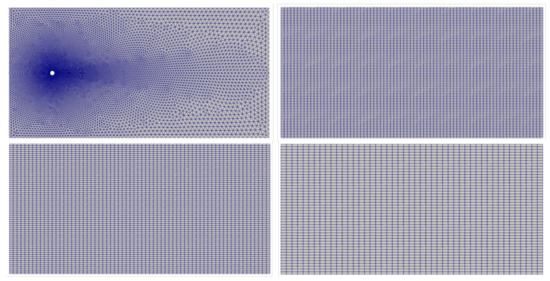
Figure 1.
On the top left, we find the high-fidelity mesh. On the top right, we find mesh n°1. On the bottom left, we find the mesh n°2. On the bottom right, we find the mesh n°3.
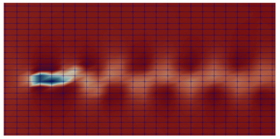
A snapshot of the first component of the velocity field is shown in Figure 2. We enlarged the grid details to show closely the flow structures and vortices past the circular cylinder.
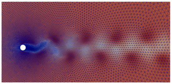
Figure 2.
An instantaneous velocity (the horizontal component) of a 2D Karman vortex street flow.
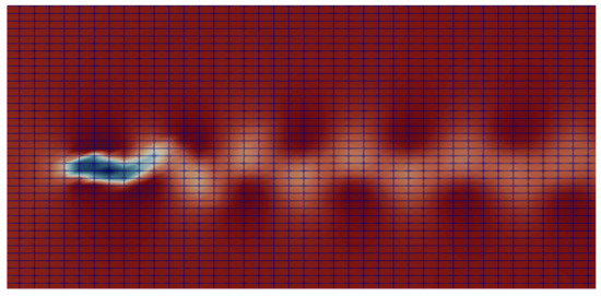
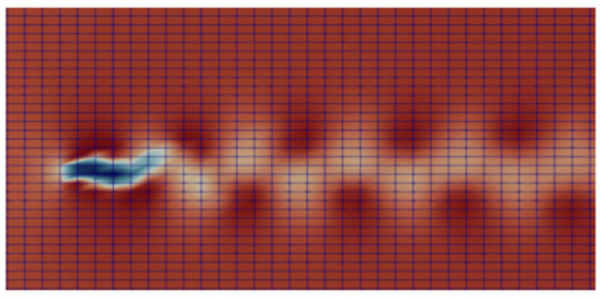
The finite element projections of the velocity field, shown in Figure 2 on the three regular meshes which are compatible with convolutional neural networks training, are shown respectively in Figure 3, Figure 4 and Figure 5.
6.2.1. Training Phase of the VAE
The training phase of the VAE or the optimization of the parameters and of the two statistical models and is performed with 998 instantaneous data or snapshots of the couple . These 998 snapshots are defined on the Cartesian mesh as stated above. They are chosen among 5000 time steps of the high-fidelity simulation corresponding to 15 s.
The architecture of the VAE is very classical; it is formed of two convolution layers and two maxpool layers followed with two fully connected layers. A nonlinear activation function is considered between the layers. The Adam optimizer [46] is considered for the optimization of the parameters and by a stochastic gradient descent. The learning rate is set equal to . The dimension of the random latent space is set equal to 3. The batch size is set equal to 20. We train the VAE during 1000 iterations.
6.2.2. POD for the Linear Reduced Order Modeling
A snapshot POD [11] is performed on the temporal correlations matrix of size from the above training set. We use this POD basis in order to make a comparison of the proposed nonlinear bayesian ROM with the classical POD-Galerkin approach for unsteady and incompressible Navier–Stokes equations. The dimension of the POD basis for the linear projection of the Navier–Stokes equations is chosen equal to 20. We specify that we do not apply any stabilization approach among the ones to which we referred in the introduction of the paper. We are using the classical POD-Galerkin method. For more information about this technique, see [47].
6.2.3. Comparison between the Nonlinear Bayesian ROM and the POD-Galerkin ROM
The offline phase of the nonlinear Bayesian ROM consists only of the training phase of the VAE over the pre-computed high-fidelity fields which are projected over the Cartesian mesh.
The offline phase of the POD-Galerkin ROM consists of the POD basis computation and the projection of the residual of the Navier–Stokes equations because of the POD approximation over each POD basis function.
The online resolution of the nonlinear Bayesian ROM combines all the steps described in the proposed algorithm. As mentioned above, the numerical efficiency is obtained thanks to the resolution of the Chorin projection method on a Cartesian mesh smaller than the unstructured one of the high-fidelity solution. This can be seen as a hyper-reduction of the nonlinear projection over the reduced random space given by h of the Navier–Stokes residual because of the manifold approximation.
The online resolution of the POD-Galerkin approach is the resolution of the reduced order dynamical system which is obtained by setting to zero the linear projection of the residual of the Navier–Stokes equations because of the POD approximation over each POD basis function, i.e., by supposing the orthogonality of the tangent space to the PDEs operators, to the POD spanned solution space.
6.2.4. Results for Mesh n°1
We first show some results of the posterior distribution learned by the VAE. In Figure 6 and Figure 7, we see respectively a scatter plot of the first two components of the parametric mean vector and the parametric logarithm of variance . The variance of the posterior distribution around the mean appears to be very small, which proves that the VAE was able to learn very sharply the training data of the couple .
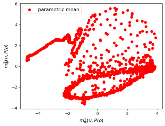
Figure 6.
Mesh n°1: The first two components of the parametrized mean of the VAE encoder.
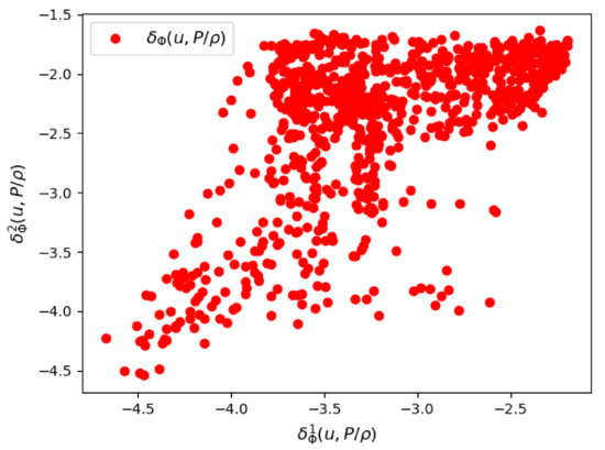
Figure 7.
Mesh n°1: The first two components of the parametrized logarithm of variance by the VAE encoder.
In Figure 8 and Figure 9, we show the mean prediction of the Bayesian nonlinear ROM at eight different spatial points with respect to time. More precisely, we show the first component of the mean prediction. This prediction is compared to the high-fidelity horizontal velocity projected on the Cartesian mesh, at the same eight spatial locations with respect to time. A confidence interval is also shown within the region of , where is the variance of the different solution samples. An extrapolation of the Bayesian nonlinear ROM solution is performed from 15 s until s. We can see in Figure 8 and Figure 9 that the mean prediction remains stable. Moreover, the confidence interval is accurate for both aggregations as it is clear in Figure 8 and Figure 9.
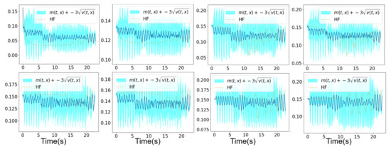
Figure 8.
Mesh n°1: High-fidelity Yales2 horizontal velocity projected on the Cartesian mesh in brown and the horizontal component of the mean prediction of the Bayesian ROM in dark blue, at eight different spatial locations. The training data correspond to s simulation time starting from s. An extrapolation is performed from s until s. The clear blue zones are the ones contained in three standard deviations around the mean prediction of the ROM denoted . The mean prediction is obtained using an aggregation of three samples of the Navier–Stokes solution by the Bayesian nonlinear ROM.
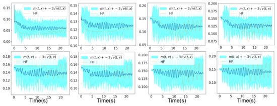
Figure 9.
Mesh n°1: High-fidelity Yales2 horizontal velocity projected on the Cartesian mesh in brown and the horizontal component of the mean prediction of the Bayesian ROM in dark blue, at six different spatial locations. The training data correspond to s simulation time starting from s. An extrapolation is performed from s until s. The clear blue zones are the ones contained in three standard deviations around the mean prediction of the ROM denoted . The mean prediction is obtained using an aggregation of 5 samples of the Navier–Stokes solution by the Bayesian nonlinear ROM.
In Figure 10, we show the first component of the unsteady velocity field at three different time instants, which corresponds to the mean prediction of the Bayesian nonlinear projection-based technique obtained with an aggregation of three solution samples. These fields are compared to the high-fidelity ones from the Yales2 solver and the ones with the POD-Galerkin ROM at the same time instants. The velocity fields with the Yales2 solver and the POD-Galerkin ROM are represented in the unstructred mesh, and the mean prediction of the Bayesian nonlinear ROM is represented on the coarse Cartesian mesh n°1.
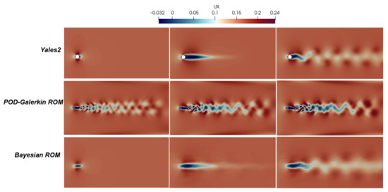
Figure 10.
Mesh n°1: On the top, the high-fidelity horizontal velocity fields in m/s by the solver Yales2. In the middle, the POD-Galerkin horizontal velocity fields in m/s. On the bottom, the horizontal velocity fields in m/s by the mean prediction of the Bayesian nonlinear ROM.
6.2.5. Results for Mesh n°2
We first show some results of the posterior distribution learned by the VAE. In Figure 11 and Figure 12, we see respectively a scatter plot of the first two components of the parametric mean vector and the parametric logarithm of variance . The variance of the posterior distribution around the mean appears to be very small, which proves that the VAE was able to learn very sharply the training data of the couple .
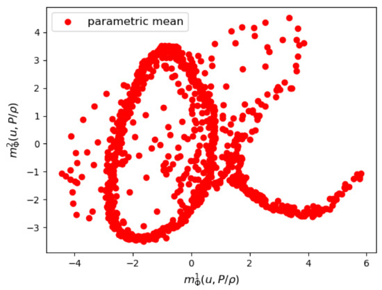
Figure 11.
Mesh n°2: The first two components of the parametrized mean of the VAE encoder.
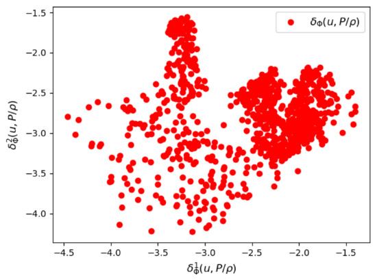
Figure 12.
Mesh n°2: The first two components of the parametrized logarithm of variance by the VAE encoder.
In Figure 13 and Figure 14, we show the mean prediction of the Bayesian nonlinear ROM at eight different spatial points with respect to time. More precisely, we show the first component of the mean prediction. This prediction is compared to the high-fidelity horizontal velocity projected on the Cartesian mesh, at the same eight spatial locations with respect to time. The temporal evolution appears to be different than the one showed in Figure 8 and Figure 9 because the time step of the Chorin method applied on mesh n°2 is larger than the one with the Chorin method applied on mesh n°1. Therefore, the comparison with the high-fidelity temporal evolution at the eight spatial points requires others high-fidelity snaphots collected at different physical times than the above study with mesh n°1, these physical times being greater. A confidence interval is also shown within the region of , where is the variance of the different solution samples. An extrapolation of the Bayesian nonlinear ROM solution is performed from s until s. The confidence interval is accurate for both aggregations as it is clear in Figure 13 and Figure 14.
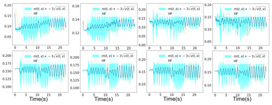
Figure 13.
Mesh n°2: High-fidelity Yales2 horizontal velocity projected on the Cartesian mesh in brown and the horizontal component of the mean prediction of the Bayesian ROM in dark blue, at eight different spatial locations. The training data correspond to s simulation time starting from s. An extrapolation is performed from s until s. The clear blue zones are the ones contained in three standard deviations around the mean prediction of the ROM denoted . The mean prediction is obtained using an aggregation of three samples of the Navier–Stokes solution by the Bayesian nonlinear ROM.
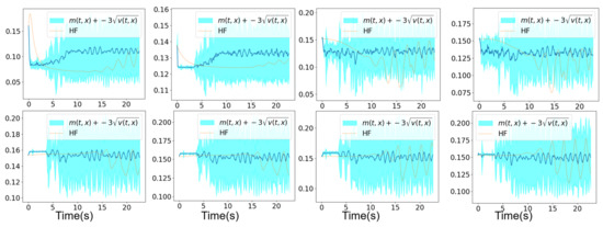
Figure 14.
Mesh n°2: High-fidelity Yales2 horizontal velocity projected on the Cartesian mesh in brown and the horizontal component of the mean prediction of the Bayesian ROM in dark blue, at eight different spatial locations. The training data correspond to s simulation time starting from s. An extrapolation is performed from s until s. The clear blue zones are the ones contained in three standard deviations around the mean prediction of the ROM denoted . The mean prediction is obtained using an aggregation of five samples of the Navier–Stokes solution by the Bayesian nonlinear ROM.
6.2.6. Results for Mesh n°3
We show the results of the posterior distribution learned by the VAE. In Figure 15 and Figure 16, we see respectively a scatter plot of the first two components of the parametric mean vector and the parametric logarithm of variance . The variance of the posterior distribution around the mean appears to be relatively small, which proves that the VAE was able to learn the training data of the couple .
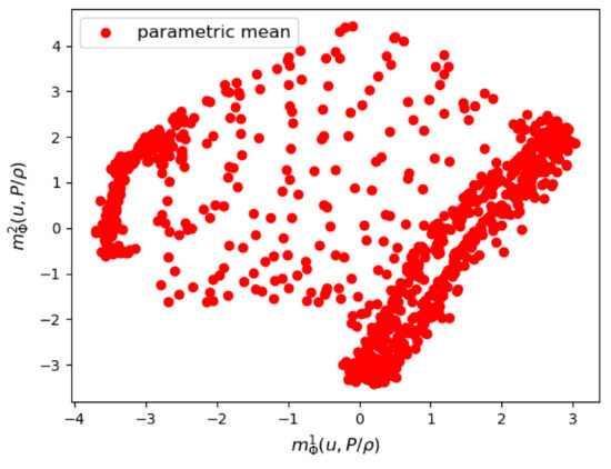
Figure 15.
Mesh n°3: The first two components of the parametrized mean of the VAE encoder.
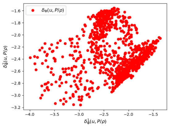
Figure 16.
Mesh n°3: The first two components of the parametrized logarithm of variance by the VAE encoder.
In Figure 17 and Figure 18, we show the mean prediction of the Bayesian nonlinear ROM at eight different spatial points with respect to time. More precisely, we show the first component of the mean prediction. This prediction is compared to the high-fidelity horizontal velocity projected on the Cartesian mesh, at the same eight spatial locations with respect to time. A confidence interval is also shown within the region of , where is the variance of the different solution samples. An extrapolation of the Bayesian nonlinear ROM solution is performed from s until s. The two predicted means respectively with three and five solution samples present an uncertainty with respect to time that the ROM confidence interval did not account for. This point will be discussed in details in the following paragraph, and it is probably related to the explicit resolution of the Navier–Stokes equations by the Chorin numerical scheme on a very coarse structured grid, which is of size for mesh n°3.
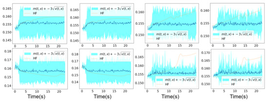
Figure 17.
Mesh n°3: High-fidelity Yales2 horizontal velocity projected on the Cartesian mesh in brown and the horizontal component of the mean prediction of the Bayesian ROM in dark blue, at eight different spatial locations. The training data correspond to s simulation time starting from s. An extrapolation is performed from s until s. The clear blue zones are the ones contained in three standard deviations around the mean prediction of the ROM denoted . The mean prediction is obtained using an aggregation of three samples of the Navier–Stokes solution by the Bayesian nonlinear ROM.
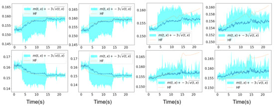
Figure 18.
Mesh n°3: High-fidelity Yales2 horizontal velocity projected on the Cartesian mesh in brown and the horizontal component of the mean prediction of the Bayesian ROM in dark blue, at eight different spatial locations. The training data correspond to s simulation time starting from s. An extrapolation is performed from s until s. The clear blue zones are the ones contained in three standard deviations around the mean prediction of the ROM denoted . The mean prediction is obtained using an aggregation of five samples of the Navier–Stokes solution by the Bayesian nonlinear ROM.
6.2.7. Discussion
We summarize in this section the main two conclusions obtained from the application of the proposed Bayesian nonlinear ROM with the three regular meshes listed in Table 1.
- We showed the sharpness of the confidence interval of the ROM mean prediction with respect to the high-fidelity solution for relatively coarse structured grids of size and . The length of this confidence interval is defined by three times the standard deviation of the solution samples.
- We showed that, for a very coarse structured mesh, which is typically of size , the confidence interval of the ROM mean prediction of a length three times the standard deviation of the solution samples could not account for the high-fidelity solution with respect to time. This means that the high-fidelity solution was outside the confidence interval sometimes. This limitation is related to the adaptive time step in the Chorin time-explicit numerical scheme, which became important for the case of mesh n°3. This time step is around s, whereas it was around s and s, respectively, for mesh n°1 and mesh n°2. The time advance of the velocity field was biased by the large time step in the mesh n°3 case. This deviation with respect to the high-fidelity solution is not taken into account within the random latent space of the VAE because the neural network learned the high-fidelity solutions (obtained with a very small adaptive time step from the Yales2 solver around s) projected on coarse structured grids.
We propose at the end of the paper a way to solve this issue.
6.3. Application to a 3D Flow in an Aeronautical Injection System
In the following section, we consider the application of the proposed reduced order modeling to a 3D unsteady, turbulent and incompressible flow in an aeronautical fuel injection system. We would like to compute the unsteady flow in the primary zone of the combustion chamber. The proposed Bayesian nonlinear reduced order model with an accurate quantification of the error bounds is an attractive way to perform such study.
The Reynolds number of this flow configuration is 45,000. A constant inlet velocity, an outlet boundary condition on the channel outlet and a wall boundary condition on the upper and lower walls of the channel are imposed. The cell number of the corresponding unstructured mesh, Figure 19, is equal to 1,700,434. The considered 3D unsteady turbulent and incompressible flow in a fuel injection system and in the primary zone of the combustion chamber is shown in Figure 20.
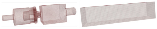
Figure 19.
On the left, we find the high-fidelity mesh. On the right, we find the coarse Cartesian mesh for the Bayesian ROM, of size .
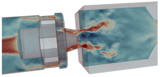
Figure 20.
A 2D plane of an instantaneous velocity (the horizontal component) of a 3D flow in the Preccinsta burner [48,49].
The finite element projection of the velocity field shown in Figure 20 on the Cartesian mesh of size , compatible with convolution neural networks, is shown in Figure 21. More precisely, we show a 2D section extracted from the horizontal component of the 3D finite element projection field.
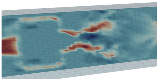
Figure 21.
A 2D plane of the finite element projection of the instantaneous velocity shown in Figure 20, on a Cartesian mesh of size .
6.3.1. Training Phase of the VAE
The training phase of the VAE is performed with 1001 instantaneous data or snapshots of the couple . These 1001 snapshots are defined on the Cartesian mesh as stated above. They are chosen among time steps of the high-fidelity simulation corresponding to s.
The architecture of the VAE is very classical, and it is formed of two convolution layers and two maxpool layers followed with two fully connected layers. A nonlinear activation function is considered between the layers. The Adam optimizer is considered for the optimization of the parameters and by a stochastic gradient descent. The learning rate is set equal to . The dimension of the random latent space is set equal to 3. The batch size is set equal to 21. We train the VAE during 1000 iterations.
6.3.2. Results
We show some results of the posterior distribution learned by the VAE. In Figure 22 and Figure 23, we see respectively a scatter plot of the first two components of the parametric mean vector and the parametric logarithm of variance . The variance of the posterior distribution around the mean appears to be relatively small, which proves that the VAE was able to sharply learn the training data of the couple .
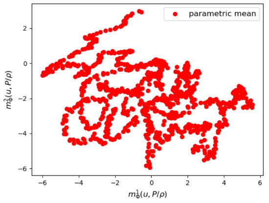
Figure 22.
The first two components of the parametrized mean of the VAE encoder.
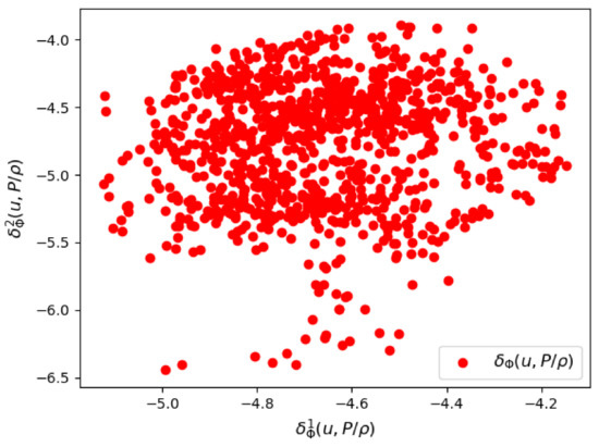
Figure 23.
The first two components of the parametrized logarithm of variance by the VAE encoder.
In Figure 24, we show the mean prediction of the Bayesian nonlinear ROM at three spatial points with respect to time. More precisely, we show the horizontal component of the mean prediction. This prediction is compared to the high-fidelity horizontal velocity projected on the Cartesian mesh, at the same spatial locations with respect to time. A confidence interval is also shown within the region of , where is the variance of the different solution samples. The confidence interval is accurate on the corresponding physical time. The ROM mean prediction is obtained with a speed-up factor up to 70 with respect to the high-fidelity solution. We obtain this efficiency in the online resolution of the nonlinear Bayesian ROM thanks to the resolution of the Chorin projection method on a coarse mesh and thanks to the fact that the unsteady solutions sampling before the aggregation is embarrassingly parallel.
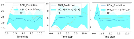
Figure 24.
High-fidelity Yales2 horizontal velocity projected on the Cartesian mesh in brown and the horizontal component of the mean prediction of the Bayesian ROM in dark blue, at three spatial points during s starting from s. The clear blue zones are the ones that are contained in three standard deviations around the mean prediction of the ROM denoted . The mean prediction is obtained using an aggregation of 10 samples of the Navier–Stokes solution by the Bayesian nonlinear ROM.
In Figure 25, we show the first component of the unsteady velocity field at instant s, which corresponds to the mean prediction of the Bayesian nonlinear projection-based technique obtained with an aggregation of 10 solution samples. This field is compared to the high-fidelity one from the Yales2 solver at the same time instant. The velocity field with the Yales2 solver is represented on the unstructured mesh and, the mean prediction of the Bayesian nonlinear ROM is represented on the coarse Cartesian mesh of size .
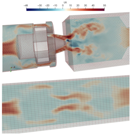
Figure 25.
On the top, a 2D plane of the high-fidelity horizontal velocity field in m/s by the solver Yales2 at s. On the bottom, a 2D plane of the horizontal velocity field in m/s by the mean prediction of the Bayesian nonlinear ROM at s.
7. Conclusions
In this paper, we have proposed a nonlinear projection based reduced order model based on variational autoencoders for the unsteady and incompressible Navier–Stokes equations. A mathematical consistency of this new formulation has been shown. This method enables a sharp analysis of the error due to the order reduction thanks to the use of Bayesian variational approaches for the prediction of the posterior distribution of the random latent (reduced) temporal coefficients associated with the nonlinear compression of an unsteady simulation. Proof of concepts of this new approach have been shown for and a test cases for the unsteady and incompressible Navier–Stokes equations. In the future, we would like to apply the proposed technique with variational autoencoders trained with different types of architectures that are more appropriate with data defined on unstructured and heterogeneous meshes. This will allow for reducing the uncertainty in the resolution of the Chorin projection method on a very coarse structured grid, more precisely the Poisson equation. This uncertainty is not taken into account within the Bayesian nonlinear ROM.
Author Contributions
Conceptualization, N.A.; methodology, N.A., F.C.; software, N.A., F.C.; validation, N.A.; formal analysis, N.A.; investigation, N.A., F.C.; resources, N.A.; data curation, N.A.; writing—original draft preparation, N.A.; writing—review and editing, F.C., E.H. and D.R.; visualization, N.A., F.C.; supervision, N.A. All authors have read and agreed to the published version of the manuscript.
Funding
This study was funded by Safran and FUI N°DOS0097899/00 MORDICUS - BPI France.
Data Availability Statement
Similar data can be reproduced using fluid dynamics softwares.
Conflicts of Interest
The authors declare no conflict of interest.
References
- Swischuk, R.; Mainini, L.; Peherstorfer, B.; Willcox, K. Projection-based model reduction: Formulations for physics-based machine learning. Comput. Fluids 2019, 179, 704–717. [Google Scholar] [CrossRef]
- Ghattas, O.; Willcox, K. Learning physics-based models from data: Perspectives from inverse problems and model reduction. Acta Numer. 2021, 30, 445–554. [Google Scholar] [CrossRef]
- Parish, E.J.; Rizzi, F. On the impact of dimensionally-consistent and physics-based inner products for POD-Galerkin and least-squares model reduction of compressible flows. arXiv 2022, arXiv:2203.16492. [Google Scholar] [CrossRef]
- Qian, E.; Kramer, B.; Peherstorfer, B.; Willcox, K. Lift & learn: Physics-informed machine learning for large-scale nonlinear dynamical systems. Phys. D Nonlinear Phenom. 2020, 406, 132401. [Google Scholar]
- Li, X.; Zhang, W. Physics-informed deep learning model in wind turbine response prediction. Renew. Energy 2022, 185, 932–944. [Google Scholar] [CrossRef]
- Zhang, R.; Liu, Y.; Sun, H. Physics-informed multi-LSTM networks for metamodeling of nonlinear structures. Comput. Methods Appl. Mech. Eng. 2020, 369, 113226. [Google Scholar] [CrossRef]
- Akkari, N.; Casenave, F.; Daniel, T.; Ryckelynck, D. Data-Targeted Prior Distribution for Variational AutoEncoder. Fluids 2021, 6, 343. [Google Scholar] [CrossRef]
- Salvador, M.; Dede, L.; Manzoni, A. Non intrusive reduced order modeling of parametrized PDEs by kernel POD and neural networks. Comput. Math. Appl. 2021, 104, 1–13. [Google Scholar] [CrossRef]
- Kwok, J.T.; Tsang, I.W. The pre-image problem in kernel methods. IEEE Trans. Neural Netw. 2004, 15, 1517–1525. [Google Scholar] [CrossRef]
- Holmes, P.; Lumley, J.; Berkooz, G.; Rowley, C. Turbulence, Coherent Structures, Dynamical Systems and Symmetry, 2nd ed.; Cambridge University Press: Cambridge, UK, 2012; pp. 358–377. [Google Scholar]
- Sirovich, L. Turbulence and the dynamics of coherent structures. Part III Dyn. Scaling Q. Appl. Math. 1987, 45, 583–590. [Google Scholar] [CrossRef]
- Iollo, A.; Lanteri, S.; Désidéri, J.A. Stability properties of POD–Galerkin approximations for the compressible Navier–Stokes equations. Theor. Comput. Fluid Dyn. 2000, 13, 377–396. [Google Scholar] [CrossRef]
- Sirisup, S.; Karniadakis, G.E. A spectral viscosity method for correcting the long-term behavior of POD models. J. Comput. Phys. 2004, 194, 92–116. [Google Scholar] [CrossRef]
- Akkari, N.; Casenave, F.; Moureau, V. Time Stable Reduced Order Modeling by an Enhanced Reduced Order Basis of the Turbulent and Incompressible 3D Navier–Stokes Equations. Math. Comput. Appl. 2019, 24, 45. [Google Scholar] [CrossRef]
- Reyes, R.; Codina, R. Projection-based reduced order models for flow problems: A variational multiscale approach. Comput. Methods Appl. Mech. Eng. 2020, 363, 112844. [Google Scholar] [CrossRef]
- Akkari, N.; Hamdouni, A.; Erwan, L.; Jazar, M. On the sensitivity of the POD technique for a parameterized quasi-nonlinear parabolic equation. Adv. Model. Simul. Eng. Sci. 2014, 1, 14. [Google Scholar] [CrossRef]
- Grimberg, S.; Farhat, C.; Youkilis, N. On the stability of projection-based model order reduction for convection-dominated laminar and turbulent flows. J. Comput. Phys. 2020, 419, 109681. [Google Scholar] [CrossRef]
- Noack, B.R.; Papas, P.; Monkewitz, P.A. The need for a pressure-term representation in empirical Galerkin models of incompressible shear flows. J. Fluid Mech. 2005, 523, 339–365. [Google Scholar] [CrossRef]
- Stabile, G.; Rozza, G. Finite volume POD-Galerkin stabilised reduced order methods for the parametrised incompressible Navier–Stokes equations. Comput. Fluids 2018, 173, 273–284. [Google Scholar] [CrossRef]
- Baiges, J.; Codina, R.; Idelsohn, S. Reduced-order subscales for POD models. Comput. Methods Appl. Mech. Eng. 2015, 291, 173–196. [Google Scholar] [CrossRef]
- Guo, M.; McQuarrie, S.A.; Willcox, K.E. Bayesian operator inference for data-driven reduced-order modeling. arXiv 2022, arXiv:2204.10829. [Google Scholar] [CrossRef]
- Goodfellow, I.; Bengio, Y.; Courville, A. Deep Learning; MIT Press: Cambridge, MA, USA, 2016; Available online: http://www.deeplearningbook.org (accessed on 1 September 2022).
- Kashima, K. Nonlinear model reduction by deep autoencoder of noise response data. In Proceedings of the 2016 IEEE 55th Conference on Decision and Control (CDC), Las Vegas, NV, USA, 12–14 December 2016; pp. 5750–5755. [Google Scholar] [CrossRef]
- Hartman, D.; Mestha, L.K. A deep learning framework for model reduction of dynamical systems. In Proceedings of the 2017 IEEE Conference on Control Technology and Applications (CCTA), Maui, HI, USA, 27–30 August 2017; pp. 1917–1922. [Google Scholar] [CrossRef]
- Lee, K.; Carlberg, K. Model reduction of dynamical systems on nonlinear manifolds using deep convolutional autoencoders. J. Comput. Phys. 2020, 404, 108973. [Google Scholar] [CrossRef]
- Kingma, D.P.; Welling, M. Auto-Encoding Variational Bayes. arXiv 2013, arXiv:1312.6114. [Google Scholar] [CrossRef]
- Chorin, A.J.; Marsden, J.E.; Marsden, J.E. A Mathematical Introduction to Fluid Mechanics; Springer Science+Business Media: New York, NY, USA, 1990; Volume 3. [Google Scholar]
- Fauque, J.; Ramière, I.; Ryckelynck, D. Hybrid hyper-reduced modeling for contact mechanics problems. Int. J. Numer. Methods Eng. 2018, 115, 117–139. [Google Scholar] [CrossRef]
- Santo, N.D.; Manzoni, A. Hyper-reduced order models for parametrized unsteady Navier–Stokes equations on domains with variable shape. Adv. Comput. Math. 2019, 45, 2463–2501. [Google Scholar] [CrossRef]
- Ryckelynck, D.; Lampoh, K.; Quilicy, S. Hyper-reduced predictions for lifetime assessment of elasto-plastic structures. Meccanica 2016, 51, 309–317. [Google Scholar] [CrossRef]
- Amsallem, D.; Zahr, M.J.; Farhat, C. Nonlinear model order reduction based on local reduced-order bases. Int. J. Numer. Methods Eng. 2012, 92, 891–916. [Google Scholar] [CrossRef]
- Mignolet, M.P.; Soize, C. Stochastic reduced order models for uncertain geometrically nonlinear dynamical systems. Comput. Methods Appl. Mech. Eng. 2008, 197, 3951–3963. [Google Scholar] [CrossRef]
- Partaourides, H.; Chatzis, S.P. Asymmetric deep generative models. Neurocomputing 2017, 241, 90–96. [Google Scholar] [CrossRef]
- Rezende, D.J.; Mohamed, S. Variational Inference with Normalizing Flows. In Proceedings of the 32nd International Conference on Machine Learning, Lille, France, 6–11 July 2015. [Google Scholar] [CrossRef]
- Caterini, A.L.; Doucet, A.; Sejdinovic, D. Hamiltonian Variational Auto-Encoder. arXiv 2018. [Google Scholar] [CrossRef]
- Joyce, J. Bayes’ Theorem. In The Stanford Encyclopedia of Philosophy, Fall 2021 ed.; Zalta, E.N., Ed.; Metaphysics Research Lab, Stanford University: Stanford, CA, USA, 2021. [Google Scholar]
- Casella, G. An Introduction to Empirical Bayes Data Analysis. Am. Stat. 1985, 39, 83–87. [Google Scholar]
- Blei, D.M.; Kucukelbir, A.; McAuliffe, J.D. Variational Inference: A Review for Statisticians. J. Am. Stat. Assoc. 2017, 112, 859–877. [Google Scholar] [CrossRef]
- Kullback, S. Information Theory and Statistics; Courier Corporation: North Chelmsford, MA, USA, 1997. [Google Scholar]
- Tran, V.H. Copula Variational Bayes inference via information geometry. arXiv 2018, arXiv:1803.10998. [Google Scholar] [CrossRef]
- Payne, L. Uniqueness and continuous dependence criteria for the Navier–Stokes equations. Rocky Mt. J. Math. 1972, 2, 641–660. [Google Scholar] [CrossRef]
- Moureau, V.; Domingo, P.; Vervisch, L. Design of a massively parallel CFD code for complex geometries. Comptes Rendus Mécanique 2011, 339, 141–148. [Google Scholar] [CrossRef]
- Moureau, V.; Domingo, P.; Vervisch, L. From Large-Eddy Simulation to Direct Numerical Simulation of a lean premixed swirl flame: Filtered laminar flame-PDF modeling. Combust. Flame 2011, 158, 1340–1357. [Google Scholar] [CrossRef]
- Malandain, M.; Maheu, N.; Moureau, V. Optimization of the deflated conjugate gradient algorithm for the solving of elliptic equations on massively parallel machines. J. Comput. Phys. 2013, 238, 32–47. [Google Scholar] [CrossRef]
- Nicolaides, R.A. Deflation of conjugate gradients with applications to boundary value problems. SIAM J. Numer. Anal. 1987, 24, 355–365. [Google Scholar] [CrossRef]
- Kingma, D.P.; Ba, J. Adam: A Method for Stochastic Optimization. arXiv 2014, arXiv:1412.6980. [Google Scholar] [CrossRef]
- Bergmann, M.; Cordier, L. Contrôle optimal par réduction de modèle POD et méthode à région de confiance du sillage laminaire d’un cylindre circulaire. Mech. Ind. 2007, 8, 111–118. [Google Scholar] [CrossRef]
- Lourier, J.M.; Stöhr, M.; Noll, B.; Werner, S.; Fiolitakis, A. Scale Adaptive Simulation of a thermoacoustic instability in a partially premixed lean swirl combustor. Combust. Flame 2017, 183, 343–357. [Google Scholar] [CrossRef]
- Franzelli, B.; Riber, E.; Gicquel, L.Y.; Poinsot, T. Large Eddy Simulation of combustion instabilities in a lean partially premixed swirled flame. Combust. Flame 2012, 159, 621–637. [Google Scholar] [CrossRef]


Publisher’s Note: MDPI stays neutral with regard to jurisdictional claims in published maps and institutional affiliations. |
© 2022 by the authors. Licensee MDPI, Basel, Switzerland. This article is an open access article distributed under the terms and conditions of the Creative Commons Attribution (CC BY) license (https://creativecommons.org/licenses/by/4.0/).