Abstract
Flow past a bluff body in freestream turbulence can substantially change the flow behaviour compared to that in smooth inflow. This paper presents the study of wake flow and aerodynamics of an oscillating square cylinder at the resonant frequency in freestream turbulence, with the integral length not greater than the cylinder side and the turbulence intensity not greater than 10%. Large eddy simulations (LES) in the Cartesian grid using the Immersed Boundary Method (IBM) technique embedded in a FVM solver, together with an efficient synthetic turbulent inflow generator implemented in an in-house parallel FORTRAN code are used for the study. The results are compared with those for smooth inflow, and relevant data published in the literature. The key findings are: the freestream turbulence conditions evidently reduces the local turbulent scales and fluctuations in the shear layer compared to in smooth flow, as small scale freestream turbulence breaks down cylinder-generated larger scale eddies and weakens them; but does not evidently affect the vortex shedding frequency, or the length of the recirculation region behind the cylinder. This suggests negligible change of drag coefficient compared to in smooth inflow. Moreover, this is because the vortex shedding is dominated by the forced oscillation at the resonance frequency, and the turbulence intensity is small.
1. Introduction
The atmospheric boundary layer (ABL) is usually turbulent. One important aspect of the freestream turbulence (FST) is its effects on flows around bluff bodies. Most of the relevant studies on FST effects were focused on stationary bluff bodies or stationary incoming flows, e.g., [1,2,3,4,5,6,7,8,9,10,11,12,13,14]. On the other hand, the ABL is never stationary, because the wind always changes direction and magnitude. The pioneering studies of non-stationary winds or oscillating bluff bodies usually considered smooth inflow only, e.g., [5,15,16,17]. Only a small number of published papers studied aerodynamics of oscillating square or rectangular cylinders in freestream turbulence, e.g., [17,18,19].
Wu and Kareem [20] reviewed studies on the vortex induced vibration (VIV) of bridge deck sections in a rectangular shape with a large width-thickness aspect ratio. They found that the turbulence effects on either the stabilization or destabilization of the VIV depended on the relative strength between Kármán vortices and motion-induced vortices. They summarized that the turbulence effects on the motion-induced force was complicated, and the deterministic effects of turbulence was to increase the vorticity diffusion and thus reduces the vortex strength. Bartoli and Righi [21] experimentally investigated the turbulence effects on the torsional flutter instability of a bridge deck section. They calculated flutter derivative and showed that the damping effect was increased with the introduction of FST. They concluded that the FST had a stabilization effect on the torsional flutter. Lin et al. [22] carried out a study of a bridge deck section in forced torsional oscillation, and their results confirmed the stabilising effect of freestream turbulence on the flutter instability.
Daniels et al. [18] and Daniels and Xie [19] studied the freestream turbulence effects on the VIV of one degree-of-freedom (DOF) motion of a bridge deck section either in heaving or torsional motion by using LES. The bridge section was a rectangular cylinder with a width-thickness ratio = 4. They extensively studied the effects of freestream turbulence intensity (TI) and integral length scale (ILS), with a focus on the responses at the resonant frequency. The stabilising effect of freestream turbulence was also found in their study as the oscillation amplitudes was reduced compared to that in smooth inflow. The increase of ILS of freestream turbulence moderately enhanced the oscillation amplitudes in both heaving and torsional motion, but all less than those for smooth inflow.
Bearman and Morel [7] and Nakamura and Ohya [9] emphasized the difficulties of drawing conclusive remarks of freestream turbulence effects on flows around a square cylinder compared to larger or smaller width-thickness ratio , in particular how large-scale turbulence affects periodical vortex shedding behind the square cylinder. They concluded that large-scale FST imposed very different impact on the cylindrical flows compared to small-scale FST, where the large scale was comparable to the cylinder thickness D, and the small scale was comparable to the shear layer thickness. In particular they noted that large-scale turbulence reduced spanwise correlation, and weakened vortex shedding behind rectangular cylinders. Lee [3], and Tamura and Ono [17] found that FST caused the leading-edge initiated shear layer to reattach intermittently on the square cylinder side, delayed the vortex formation, and effectively lengthened the recirculation region in the wake, whereas many other studies found that it shortened the recirculation region behind a flat-plate or a rectangular cylinder (e.g., ). This highlights the importance of studying FST effects on the aerodynamics of a square cylinder, in particular the FST length scale. Bearman and Morel [7] commented that ‘there is not such an easy rule of thumb for the effects of the length scale’, suggesting the difficulties.
It is perhaps not suprising that no conclusive remarks haven been drawn so far for the FST effects on the response at resonance of an oscillating square cylinder. Experimental data [5] showed that the structure response at Scruton number was not influenced by the FST with the turbulence intensity , and the dimensionless integral length scale . At and in the same FST condidtions, the amplitude of the response was evidently increased compared to that in smooth inflow. Numerical data [17] showed the FST had a little effect on the onset of unstable oscillations for a square cylinder at with and . However, at and in the same FST condidtions, the amplitude of the response near the onset velocity increased in comparison to in smooth inflow.
It is crucial to note that the FST length scales studied in the literature were not significantly greater than the width in streamwise direction of the rectangular cylinder (e.g., bridge section), e.g., [18,21,22]. This is perhaps because simulations of very large FST length scales challenge the experimental and numerical designs. This again leaves the effect of FST length scale an open question.
Our previous study [23] investigated aerodynamics of stationary and oscillating square cylinders in a smooth incoming flow. This paper is focused on the effects of FST on a forced oscillating square cylinder at the resonant frequency, and a Reynolds number of 22,000 based on bulk incoming velocity and cylinder side length D. Different turbulence intensity () and integral length scale () were considered. The rest of paper is organised as follows. The numerical methods are introduced in Section 2, including the governing equations and the synthetic turbulence generation (STG) method. The implementation of the STG method is validated by using a single slice of inflow plane in Section 3. The numerical setup of a forced oscillating square cylinder in freestream turbulence is introduced in Section 4. The results and their analysis are presented in Section 5. The conclusion is presented in Section 6.
2. Numerical Methods
2.1. Governing Equations
The incompressible flow governing equations of LES are shown below,
where and p are resolved velocity and pressure, respectively, is density, is sub-grid scale (SGS) stress. The mixed time scale SGS model [24] is used to model the SGS stress terms, with the two parameters and . The explicit second order Adam-Bashforth method is used for temporal discretisation. For the spatial discretisation, the second order central difference scheme is used for the diffusion term, and the third order QUICK scheme [25] is used for the convection term. The computations were conducted in a Cartesian grid. To model a solid body, an immersed boundary method (IBM) [26] was used. The developed flow solver in FORTRAN was extensively tested [23] for aerodynamics of stationary and forced oscillating square cylinders in a smooth incoming flow.
2.2. Turbulent Inflow Generation
To generate homogeneous isotropic turbulence (HIT), a rigorously tested STG [27,28] is implemented in the flow solver. Compared to other alternative synthetic turbulence generation approaches, it is efficient and is able to produce an inertial subrange in spectrum [29,30], which allows it being capable for large Reynolds number flows, e.g., [31]. The STG is based on exponential correlations in space and in time, which significantly increases the efficiency. The imposed correlations satisfy the prescribed integral length and time scales.
For the readers’ convenience, a brief of the STG is given here. The instantaneous velocity at the inlet is decomposed into the mean and fluctuating velocities:
where , and is an amplitude tensor and is an unscaled fluctuation with a zero mean and unit variance. Lund et al. [32] suggested that a form for amplitude tensor can be written using Cholesky decomposition of Reynolds stress tensor as
For homogeneous isotropic turbulence, the cross-correlation terms , and the diagonal terms .
To illustrate this filtering process, a set of discretised 1D velocity fluctuations on a uniform grid are used and they can be calculated,
where is a series of random data with zero mean and unit variance, are filter coefficients, N is related to the integral length scale of filter and . An autocorrelation function of velocity fluctuation with integral length scale L, and distance apart of two grid points on the 1D uniformly discretised mesh is calculated,
where is grid spacing and subscript m denotes the discretised spatial location of the variable. The filter coefficients are calculated,
It is straightforward to expand the 1D fluctuation in Equation (5) to generate velocity fluctuations on a 2D space as
where are associated with the integral length scales in the two directions, respectively.
Only one additional 2D slice of data (Equation (7)) is generated at every new time step. A forward-stepwise method is used to correlate two successive time-step data (Equation (8)),
where t and are current and next time steps. is a 2D slice of fluctuations obtained from Equation (7). T is the Lagrangian time scale.
2.3. Boundary Conditions
The synthetic turbulence was imposed in the region at the inlet (Figure 1a and Figure 2), which fully accommodated the shear layer over the side surfaces of square cylinder and the near wake. This was to avoid resolving small turbulent eddies in the regions far away from the cylinder and to further improve the computational efficiency, albeit an efficient STG was used. Such a simple treatment of the inlet settings might have an effect on the far wake flow, nevertheless its effect on the cylinder, the shear layer and the near wake was negligible. Uniform velocities were imposed at the rest of the inlet. It was ensured that entire inlet has the same mean velocity. Outflow boundary condition with zero gradient in the boundary-normal direction was applied at the outlet. Symmetric boundary conditions were used on the top and bottom boundaries of the domain. In the spanwise direction, periodic boundary conditions were used. No-slip boundary condition was applied on the square cylinder surfaces by using the extensively tested immersed boundary method [23]. The distance between the centre of cylinder and the inlet is , which was suggested in [33], being a compromise of turbulence development distance and computational cost. Within such a distance, the changes of the and were small.
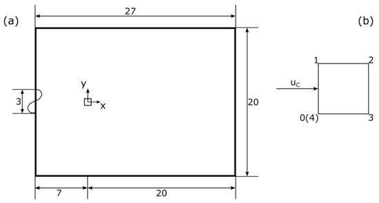
Figure 1.
(a) Computational domain and the dimensions normalised by the side length of cylinder D; (b) Definition of circumferential direction of a cylinder section. The coordinate origin is placed on the centre of the cylinder.
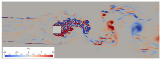
Figure 2.
Contours of instantaneous spanwise vorticity over a stationary cylinder. , .
3. Validation of the Implementation of Turbulent Inflow Generation Method
To validate the implementation of turbulent inflow generation, a homogeneous isotropic turbulence case was tested on a 2D plane with a uniform mesh. Auto-correlations and two-point correlations were computed from the sampled velocity fluctuations.
The dimensionless parameters of the uniform mesh are listed as follows. The grid cell number is with grid spacing . The convection velocity . Mean vertical and spanwise velocity components . The integral length scales in three directions are , and the equivalent Lagrangian time scale . The Reynolds normal stress are . The virtual streamwise grid spacing is . The time step is and the CFL number is .
The time series of three velocity components are sampled at the central point of the plane. The power spectrum densities (PSD) of the three velocity components are shown in Figure 3. For the sake of clarity, the v and w spectra are shifted down by 2 and 4 decades, respectively. The three spectra shows an evident slope, indicating a wide inertial subrange. This suggests that the generated synthetic turbulence can be used for high Reynolds number flow problems.
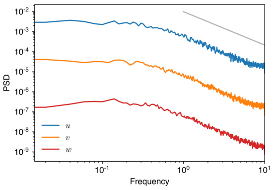
Figure 3.
PSD of three velocity components collected at the centre of inflow plane. For the sake of clarity, the v and w spectra are shifted down by 2 and 4 decays, respectively. The grey line denotes a slope of −5/3.
Figure 4 shows two-point correlations of vertical (v) and spanwise velocity (w) components at the central horizontal line. The analytical exponential correlation is obtained from Equation (6). It is to be noted that the convection distance in streamwise direction is computed as . Figure 4 shows that correlations of the synthetic turbulence are in good agreement with the exponential correlation function.
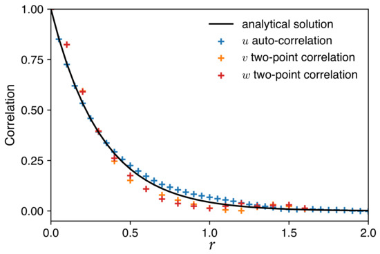
Figure 4.
Two-point correlations for two velocity components v and w on the central horizontal line, and auto-correlation for velocity component u. The black line denotes the analytical exponential correlation for the same integral length scale and the equivalent integral time scale.
4. Numerical Setup
4.1. Domain Configuration and Resolution Verification
A forced oscillating square cylinder in freestream turbulence is studied. The Reynolds number based on the mean inflow velocity and cylinder side length D is 22,000. The computational domain and the definition of circumferential direction of section of the square cylinder are shown in Figure 1. The dimensionless lengths of computational domain are in streamwise x, vertical y and spanwise z directions, respectively, which are normalized by the side length D of the square cylinder.
Sensitivity tests for spatial and temporal resolutions were carried out and reported in [23,34], in which several various resolutions were investigated. These concluded that the results, i.e., the Strouhal number , the aerodynamic force coefficient , and fluctuating force coefficients for the medium and the fine resolutions were within a small tolerance. The fine mesh was rigorously validated in the smooth inflow past a square cylinder at Reynolds number 22,000 case in [23].
The fine mesh was chosen in this paper, which had a uniform resolution in to capture the flow details in the near cylinder region, which was 200 points per side length D resulting in a maximum less than 5. The mesh was stretched in the vertical direction from the region to the top and bottom boundaries with a maximum stretch ratio less than 1.02. The mesh in spanwise direction was uniform. A total number of 736 (streamwise) × 1152 (vertical) × 64 (spanwise) cells is used.
A non-dimensional time step was used in all simulations, which yielded the maximum number less than 0.3. An initialisation duration of LES was , where was the oscillation period (Equation (9)). A further duration of LES was carried out for sampling data. It is to be noted that the oscillation period was 7.7 times the the flow pass-through time ( ). The selected initialisation and sampling durations produced statistically converged data.
The computational domain is decomposed into partitions for parallel computation. The identical setup of computational domain and decomposition is used through all the remaining cases in this paper.
4.2. One-Degree-of-Freedom Oscillation of the Cylinder
The one-degree-of-freedom oscillation of the square cylinder was perpendicular to the inflow. The time varying displacement in vertical direction (y) is written,
where A is amplitude, f is frequency. To understand the freestream turbulence effects on aerodynamics of an oscillating square cylinder in extreme scenarios, the resonant reduced velocity [15] was applied in the simulations with an amplitude ratio . When the reduced velocity is equal or close to the resonant reduced velocity, the vortex shedding frequency is locked to the resonant frequency of the structure. This phenomenon is known as ‘lock-in’ or ‘synchronization’. For modeling a forced oscillating cylinder compared to a freely oscillating cylinder, the advantages are that the flow parameters are under well-control, and the experimental or numerical cost is much less. Bearman and Obasaju (1982) [15] concluded that the flow features were very close to those of freely oscillating cylinder when the basic parameters were matched.
4.3. Freestream Turbulence Parameters
Bearman and Morel (1983) [7] suggested that the investigated length scales “should be somewhere in the range between one order of magnitude smaller than the shear layer thickness, and one order of magnitude larger than the typical body dimension”. They also stated that no consistent relationship was found between the integral length scale and the typical body dimension in a range of . Several published studies, e.g., [9,17,18] investigated the similar range of values and were not yet able to draw a conclusive remark. In the present work three turbulent inflow cases, (1) , , (2) , , and one smooth inflow case were studied. For the large freestream turbulence scale in case 1, the equivalent integral time scale () was , which was one order of magnitude smaller than the oscillation period (i.e., ). For the small freestream turbulence scale in case 2, the equivalent was two orders of magnitude smaller than the oscillation period (i.e., ). A distinct time-scale separation between the FST and the oscillation helped to identify the effect of FST.
5. Flow Past an Oscillating Square Cylinder
5.1. Fluctuating Lift and Its Power Spectrum Distribution
Figure 5 shows the power spectrum distribution (PSD) of lift coefficients of three turbulent inflow cases against frequency ratio , where is the forced oscillation frequency. The gray solid line indicates the forced oscillation frequency . The three curves show that an evident synchronization occurs at , indicating that the synchronization is not affected by inflow conditions. As discussed in Section 4, the time scales of the energetic turbulent eddies are one or two orders of magnitude smaller than the time scale of resonance. This suggests that the vortex shedding at lock-in is more dominated by the heaving motion than the FST disturbance at , or in other words, the FST’s impact is decoupled with the much slower forced oscillation.
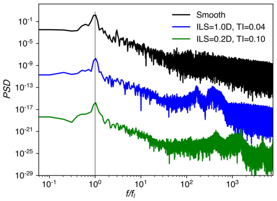
Figure 5.
PSD of lift coefficients against frequency ratio . The spectra of “, ” and “, ” are shifted down in the vertical axis by 8 and 16 decades, respectively.
Greater PSD at two orders of magnitude larger than frequencies is visible in the two turbulent inflow cases, compared to that in the smooth flow case. This is due to the impact of high-frequency FST. This impact is on turbulence scales smaller than the shear-layer thickness. It is to be noted that the PSD has very low values at these frequencies compared to , and perhaps it is not worth paying too much attention on this.
A typical time series of instantaneous lift coefficient was much “rougher” showing small-scale fluctuations for the FST cases compared to the smooth inflow case. This is due to the so-called turbulent buffeting effect, and is consistent with the larger PSD at high frequencies for the FST cases compared to the smooth inflow case showing in Figure 5. Bearman and Obasaju [15] showed that the phase angle difference between the lift coefficient and displacement had a significant change at the resonant frequency indicating a large uncertainty, in particular for a small oscillation amplitude . We did noticed this large uncertainty in our current and previous studies [23].
Overal, the small scale FST (i.e., ) has little impact on the lift PSD for the forced oscillating cylinder. This is consisten with those for a rectangular cylinder in small scale FST [18,19], in which they concluded that the FST evidently reduced the response. Miyazaki and Miyata [5] and Tamura and Ono [17] studied the response of a square cylinder in the FST with larger integral length scales (), found only in a small range of the Scruton number the amptitude of the response was evedently increased.
5.2. Spatial Correlation in the Shear Layer and the Wake
Figure 6 shows contours of two-point correlation of streamwise velocity in the shear layer and the wake. The data were sampled from an plane, where a reference point (, ) was selected. These were similar to the settings in [35]. The contour range was from 0 (in dark blue) to 1 (in dark red) with an increment 0.1, where the nagative data of correlation was truncated. It was evident that the length scales in both x and y directions were reduced in the FST compared to those in smooth inflow. This was because the studied integral length scales of the FST were about one order of magnitude smaller than the fluid particle travelling distance during one period of the forced oscillation. In other words, the studied integral time scales of the FST were much smaller than the oscillation period. Subsequently the FST reduced the integral length scales in the shear layer and wake regions. This is in agreement with those for a rectangular cylinder in small scale FST [18,19]. The length scales in Figure 6b for are slightly larger than those in Figure 6c for , which perhaps is because the greater scales in the FST.
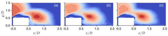
Figure 6.
Two-point correlation of streamwise velocity. The reference point is at , . (a) smooth inflow, and turbulent inflows with (b) , , and (c) , . Contours starts from 0 (in dark blue) to 1 (in dark red) with an increment 0.1.
Figure 7 shows two-point correlations of streamwise velocity along the spanwise direction at 3 locations: wake (, ), shear layer in the wake (, ) and shear layer over side surfaces (, ). At the two shear layer stations, it is evident that the correlation length is reduced for the two FST cases compared to the smooth inflow case. This confirms the remark from Figure 6 that the FST reduces the turbulent length scales in the shear layer in all 3 directions. The spanwise length scales for are slightly larger than for at these two stations. At the wake station, the FST yields no visible difference in spanwise correlation. This might be because the FST cannot entrain far enough to this region, where the flow is mostly shielded from the FST.
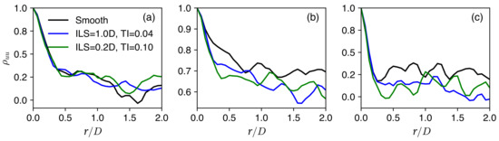
Figure 7.
Spanwise correlation of streamwise velocity. The locations of a group of spanwise probes from left to right are at (a) wake, , , (b) shear layer in the wake, , , and (c) shear layer over the side surfaces, , .
5.3. Turbulent Statistics and Recirculation in the Wake
Figure 8 shows contours of the time- and spanwise-averaged Reynolds normal stress . The FST significantly reduces the turbulent fluctuations in the shear layer. In the regions near the wind-ward side and near the central plane in the wake, and in the far wake, the FST increases the turbulent fluctuations due to turbulent entrainment and mixing. No visible difference in was observed between the two FST cases. This was because the turbulent fluctuations produced by the cylinder itself was much greater than those in the FST. Again, it is to be noted the oscillation time period was much greater than the FST integral time scale.
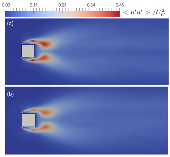
Figure 8.
Time and spanwise-averaged Reynolds normal stress . (a) smooth inflow; (b) ILS = 0.2D, TI = 0.10.
Figure 9 shows that the difference of the recirculation lengths between smooth and FST cases is negligible. This suggests that the recirculation in the wake is dominated by the resonant oscillation, while the FST with a integral length scale not greater than D has no visible impact on the recirculation length. This differs from the FST effects on the recirculation length of a stationary square cylinder [7,17]. Tamura and Ono [17] found that the FST with increased the length of the recirculation region behind a circular cylinder, which was consistent with the evidently reduced drag in the FST () reported in Courchesne [6]. Therefore, even though the oscillation time period was one order of magnitude greater than the FST integral time scale, the oscillation cannot be considered as a quasi-stationary state in terms of the FST interaction.
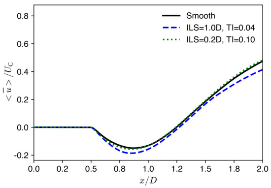
Figure 9.
Time- and spanwise-averaged streamwise velocity on the central horizontal plane.
6. Conclusions and Discussion
Up to the authors’ knowledge, so far there is no conclusive remarks on the freestream turbulence effect on a stationary or oscillating square cylinder, in particular on the role of the FST integral length scale. The current study addresses the effect of FST with the integral length scales on a forced oscillating square cylinder at the resonance frequency, and aims to drawing conclusive remarks.
For the square cylinder in forced oscillation at the resonant frequency, we found that the vortex shedding was not evidently affected by the FST with the turbulence intensity (i.e., 10%) and integral length scales (i.e., ). We also noticed that the length of the recirculation region behind the square cylinder was not evidently affected by the FST, suggesting a negligible change of drag coefficient compared to in smooth inflow. This was because the vortex shedding was dominated by the forced oscillation at the resonance frequency, and turbulence intensity was small.
Our numerical simulations show that the local turbulence integral length scales were evidently reduced in the shear layer in the FST compared to in smooth flow. The FST significantly reduced the turbulent fluctuations in the shear layer. This was because the FST small scale turbulence broke down the cylinder generated larger scale eddies and weakened them, and was consistent with that for a stationary cylinder in small scale freestream turbulence. On the other hand, in the regions near the wind-ward side, near the central plane in the wake, and in the far wake, the FST enhanced the local turbulence. This was because the freestream turbulence was entrained or convected into these regions, again was consistent with for a stationary cylinder. It is to be noted that the FST integral time scales were at least one-order-of-magnitude smaller than the period of the forced oscillation, and the FST was somehow decoupled with the vortex shedding at the resonant frequency.
It is crucial to note that the FST with length scales smaller than the width (i.e., the dimension in streamwise direction) of a bridge deck (i.e., a large aspect ratio rectangular cylinder) stabilises the heaving or torsional motions, e.g., [18,21,22]. This is because the FST breaks down the leading-edge initiated vortex, and weakens the in-phase vortex shedding in the spanwise direction. As for an oscillating square cylinder at the resonance frequency in freestream turbulence, the priority in future work is to understand the impact of the large scale FST (e.g., ). Greater turbulence intensity (e.g., ) and greater oscillation amplitude ration () should be considered too.
Author Contributions
Conceptualization, Y.C. and Z.-T.X.; methodology, Y.C. and Z.-T.X.; software, Y.C. and Z.-T.X.; validation, Y.C. and Z.-T.X.; formal analysis, Y.C. and Z.-T.X.; investigation, Y.C., K.D. and Z.-T.X.; resources, Y.C. and Z.-T.X.; data curation, Y.C.; writing—original draft preparation, Y.C. and Z.-T.X.; writing—review and editing, K.D. and Z.-T.X.; visualization, Y.C.; supervision, K.D. and Z.-T.X.; project administration, Z.-T.X.; funding acquisition, Z.-T.X. All authors have read and agreed to the published version of the manuscript.
Funding
The authors would like to thank EPSRC for the computational time made available on the UK supercomputing facility ARCHER via the UK Turbulence Consortium (EP/L000261/1 for the old grant 2013–2018 and EP/R029326/1 for the new grant 2018–2022). Z.-T.X. is grateful to the EPSRC grant EP/V010514/1 for funding their time contributing to completion of the paper.
Data Availability Statement
Not applicable.
Acknowledgments
The authors also thank the HPC facility IRIDIS at the University of Southampton. Yongxin Chen thanks the Rayleigh international studentship from the University of Southampton.
Conflicts of Interest
The authors declare no conflict of interest.
References
- Vickery, B. Fluctuating lift and drag on a long cylinder of square cross-section in a smooth and in a turbulent stream. J. Fluid Mech. 1966, 25, 481–494. [Google Scholar] [CrossRef]
- Mulhearn, P. Stagnation and reattachment lines on a cylinder of square cross-section in smooth and turbulent flows. Nat. Phys. Sci. 1973, 241, 165–167. [Google Scholar] [CrossRef]
- Lee, B. The effect of turbulence on the surface pressure field of a square prism. J. Fluid Mech. 1975, 69, 263–282. [Google Scholar] [CrossRef]
- Castro, I.; Robins, A. The flow around a surface-mounted cube in uniform and turbulent streams. J. Fluid Mech. 1977, 79, 307–335. [Google Scholar] [CrossRef]
- Miyazaki, M.; Miyata, T. Effect of turbulence scale on aerodynamic responses of rectangular cylinders. In Proceedings of the 5th Symposium Wind Eff. Struct, Tokyo, Japan, December 1978; pp. 191–198. [Google Scholar]
- Courchesne, J. Rectangular section cylinders subjected to low-turbulence and turbulent two-dimensional flows. In Proceedings of the Second Canadian Workshop on Wind Engineering: l’Institut de Recherche de l’Hydro-Quebec (IREQ), Varennes, QC, Canada, 28–29 September 1978. [Google Scholar]
- Bearman, P.; Morel, T. Effect of free stream turbulence on the flow around bluff bodies. Prog. Aerosp. Sci. 1983, 20, 97–123. [Google Scholar] [CrossRef]
- Laneville, A.; GV, P. An explanation of some effects of turbulence on bluff bodies. In Proceedings of the Fourth International Conference on Wind Effects on Buildings and Structures, London, UK, 8–12 December 1975; pp. 333–341. [Google Scholar]
- Nakamura, Y.; Ohya, Y. The effects of turbulence on the mean flow past two-dimensional rectangular cylinders. J. Fluid Mech. 1984, 149, 255–273. [Google Scholar] [CrossRef]
- Daniels, S.J.; Castro, I.P.; Xie, Z.T. Peak loading and surface pressure fluctuations of a tall model building. J. Wind. Eng. Ind. Aerodyn. 2013, 120, 19–28. [Google Scholar] [CrossRef]
- Yan, B.; Li, Q. Inflow turbulence generation methods with large eddy simulation for wind effects on tall buildings. Comput. Fluids 2015, 116, 158–175. [Google Scholar] [CrossRef]
- Ricci, M.; Patruno, L.; de Miranda, S.; Ubertini, F. Flow field around a 5:1 rectangular cylinder using LES: Influence of inflow turbulence conditions, spanwise domain size and their interaction. Comput. Fluids 2017, 149, 181–193. [Google Scholar] [CrossRef]
- Xia, J.; Li, K.; Ge, Y. Spanwise coherence of fluctuating forces on twin bridge decks and the turbulence effect. Adv. Struct. Eng. 2019, 22, 3207–3221. [Google Scholar] [CrossRef]
- Zhao, C.; Wang, H.; Zeng, L.; Alam, M.M.; Zhao, X. Effects of oncoming flow turbulence on the near wake and forces of a 3D square cylinder. J. Wind. Eng. Ind. Aerodyn. 2021, 214, 104674. [Google Scholar] [CrossRef]
- Bearman, P.; Obasaju, E. An experimental study of pressure fluctuations on fixed and oscillating square-section cylinders. J. Fluid Mech. 1982, 119, 297–321. [Google Scholar] [CrossRef]
- Taylor, I.; Vezza, M. Calculation of the flow field around a square section cylinder undergoing forced transverse oscillations using a discrete vortex method. J. Wind. Eng. Ind. Aerodyn. 1999, 82, 271–291. [Google Scholar] [CrossRef]
- Tamura, T.; Ono, Y. LES analysis on aeroelastic instability of prisms in turbulent flow. J. Wind. Eng. Ind. Aerodyn. 2003, 91, 1827–1846. [Google Scholar] [CrossRef]
- Daniels, S.J.; Castro, I.P.; Xie, Z.T. Numerical analysis of freestream turbulence effects on the vortex-induced vibrations of a rectangular cylinder. J. Wind. Eng. Ind. Aerodyn. 2016, 153, 13–25. [Google Scholar] [CrossRef]
- Daniels, S.J.; Xie, Z.T. An overview of Large-Eddy Simulation for wind loading on slender structures. Proc. Inst. Civ.-Eng.-Eng. Comput. Mech. 2022, 175, 1–67. [Google Scholar] [CrossRef]
- Wu, T.; Kareem, A. An overview of vortex-induced vibration (VIV) of bridge decks. Front. Struct. Civ. Eng. 2012, 6, 335–347. [Google Scholar] [CrossRef]
- Bartoli, G.; Righi, M. Flutter mechanism for rectangular prisms in smooth and turbulent flow. J. Wind. Eng. Ind. Aerodyn. 2006, 94, 275–291. [Google Scholar] [CrossRef]
- Lin, Y.Y.; Cheng, C.M.; Wu, J.C.; Lan, T.L.; Wu, K.T. Effects of deck shape and oncoming turbulence on bridge aerodynamics. Tamkang J. Sci. Eng. 2005, 8, 43–56. [Google Scholar]
- Chen, Y.; Djidjeli, K.; Xie, Z.T. Large eddy simulation of flow past stationary and oscillating square cylinders. J. Fluids Struct. 2020, 97, 103107. [Google Scholar] [CrossRef]
- Inagaki, M.; Kondoh, T.; Nagano, Y. A mixed-time-scale SGS model with fixed model-parameters for practical LES. J. Fluids Eng. 2005, 127, 1–13. [Google Scholar] [CrossRef]
- Leonard, B.P. A stable and accurate convective modelling procedure based on quadratic upstream interpolation. Comput. Methods Appl. Mech. Eng. 1979, 19, 59–98. [Google Scholar] [CrossRef]
- Yang, J.; Balaras, E. An embedded-boundary formulation for large-eddy simulation of turbulent flows interacting with moving boundaries. J. Comput. Phys. 2006, 215, 12–40. [Google Scholar] [CrossRef]
- Xie, Z.T.; Castro, I.P. Efficient generation of inflow conditions for large eddy simulation of street-scale flows. Flow Turbul. Combust. 2008, 81, 449–470. [Google Scholar] [CrossRef]
- Kim, Y.; Castro, I.P.; Xie, Z.T. Divergence-free turbulence inflow conditions for large-eddy simulations with incompressible flow solvers. Comput. Fluids 2013, 84, 56–68. [Google Scholar] [CrossRef]
- Wu, X. Inflow Turbulence Generation Methods. Annu. Rev. Fluid Mech. 2017, 49, 23–49. [Google Scholar] [CrossRef]
- Bercin, K.; Xie, Z.; Turnock, S. Exploration of digital-filter and forward-stepwise synthetic turbulence generators and an improvement for their skewness-kurtosis. Comput. Fluids 2018, 172, 443–466. [Google Scholar] [CrossRef]
- Klapwijk, M.; Lloyd, T.; Vaz, G.; Van Terwisga, T. Evaluation of scale-resolving simulations for a turbulent channel flows. Comput. Fluids 2020, 209, 1–20. [Google Scholar] [CrossRef]
- Lund, T.S.; Wu, X.; Squires, K.D. Generation of turbulent inflow data for spatially-developing boundary layer simulations. J. Comput. Phys. 1998, 140, 233–258. [Google Scholar] [CrossRef]
- Kim, Y.; Xie, Z.T. Modelling the effect of freestream turbulence on dynamic stall of wind turbine blades. Comput. Fluids 2016, 129, 53–66. [Google Scholar] [CrossRef]
- Chen, Y.; Djidjeli, K.; Xie, Z.T. Large eddy simulation of flow past a bluff body using immersed boundary method. In Proceedings of the 25th Anniversary of the European Community on Computational Methods in Applied Sciences (ECCOMAS), Glasgow, UK, 11–15 June 2018. [Google Scholar]
- Coletti, F.; Maurer, T.; Arts, T.; Di Sante, A. Flow field investigation in rotating rib-roughened channel by means of particle image velocimetry. Exp. Fluids 2012, 52, 1043–1061. [Google Scholar] [CrossRef]


Publisher’s Note: MDPI stays neutral with regard to jurisdictional claims in published maps and institutional affiliations. |
© 2022 by the authors. Licensee MDPI, Basel, Switzerland. This article is an open access article distributed under the terms and conditions of the Creative Commons Attribution (CC BY) license (https://creativecommons.org/licenses/by/4.0/).