Abstract
Lattice Boltzmann method (LBM) simulations were performed to capture the long-period dynamics within the wake of a realistic DrivAer fastback model with stationary and rotating wheels. The simulations showed that the wake developed as a low-pressure torus regardless of whether the wheels were rotating. This torus shrank in size on the base in the case of rotating wheels, leading to a reduction in the low-pressure footprint on the base, and consequently a decrease in the total vehicle drag in comparison to the stationary wheels case. Furthermore, the lateral vortex shedding experienced a long-period switching associated with the bi-stability in both the stationary and rotating wheels cases. This bi-stability contributed to low-frequency side force oscillations (<1 Hz) in alignment with the peak motion-sickness-inducing frequency (0.2 Hz).
1. Introduction
Simplified square-back automotive models such as the Ahmed body [1] and the Windsor body [2] have been found to develop aperiodic vortex shedding wherein the shedding of vortices favors one side of the vehicle over long time periods [2,3,4,5,6,7,8,9,10,11,12,13,14,15,16,17,18]. This aperiodic wake-switching behavior is typically referred to as bi-stability. The bi-stabiltiy is responsible for as much as of the vehicle drag [11]. Additionally, the bi-stability is associated with a long time period, ranging from 1 to 10 s [4]. Such long-period oscillations have been found to induce motion sickness [19,20,21,22,23,24], which could negatively affect vehicle occupants. Mitigation of the bi-stability and its subsequent effects has been effective through both passive and active flow control methods on simplified automotive models. Passive flow control techniques, such as the addition of a cavity on the vehicle base, successfully suppress the low-frequency switching of the bi-stability, reducing the vehicle drag [13]. Active flow control, such as oscillating flaps on the edge of the base, suppress the bi-stability and improve vehicle drag as well [12]. However, neither method has gained acceptance for an actual car. The lack of a realistic representation of production cars when using simplified automotive models has limited an effective extrapolation of such flow control studies to production vehicles.
Attempts have been made to rectify the issue of oversimplification by analyzing the effects of additional vehicle model complexity on the bi-stability of the wake flow. One obvious extra level of realism has been the addition of wheels. However, even for simplified square-back automotive models, the impact of wheels on wake bi-stability has not been conclusive. On one hand, Pavia et al. [4] and Pavia and Passmore [2] reported that adding stationary wheels to a Windsor body eliminated the bi-stability, resulting in a short-time swinging of the wake. On the other hand, Grandemange et al. [25] found that the bi-stability persisted in the wake of an Ahmed body when rotating wheels are added. Such an inconsistency may suggest a significant impact of wheel rotation on the development of bi-stability in the wake flow, in addition to the vehicle geometry itself. Vehicle geometry has been shown previously to impact the structure of the bi-stability on simplified square-back models [26]. Additionally, the bi-stability has even been observed for production vehicles with rotating wheels (albeit at non-zero yaw angles) [27,28]. However, no studies exist thus far that have directly compared wake dynamics and bi-stability for a single realistic vehicle with and without wheel rotation.
For the current work, our goal is to characterize the effect of wheel rotation on the wake dynamics for a realistic automotive model to better inform future flow control studies. The realistic model considered is the fastback DrivAer model [29] (Section 2.1). To capture the flow field, we used lattice Boltzmann method (LBM) simulations due to their computational efficiency for automotive flows [30]. Details on the numerical setup used are given in Section 2, such as the domain and boundary conditions (Section 2.2), mesh setup (Section 2.3), and general parameters for the LBM simulations (Section 2.4). Results and discussions are reported in Section 3, including an assessment of the time-averaged flow to confirm the validity of the simulations (Section 3.1) and a detailed characterization of the long-period wake dynamics in the context of stationary and rotating wheels (Section 3.2). The major findings and conclusions are briefly described in Section 4.
2. Methodology
2.1. DrivAer Model
Until recently, most automotive aerodynamic studies focused on two types of vehicle models: simplified models like the classical Ahmed body or production vehicles. Models such as the Ahmed body have been heavily studied and capture some of the basic flow structures, such as the separated wake and trailing vortex system. While these simple geometries make great test beds for fundamental research of basic automotive flow structures, they fail to represent real automotive vehicles. Rotating wheels, side mirrors, and complex underbodies are just some of the geometric features that these simplified models lack. On the other hand, production vehicles have no simplifications whatsoever. Unfortunately, these geometries vary heavily across markets and time, making transfer of knowledge difficult across both academia and industry. To bridge the gap between simplified models and production vehicles, Technische Universität München (TUM) developed a realistic car model known as the DrivAer model and made it publicly available. The DrivAer model is a combination of the Audi A4 and BMW 3 Series. It is a highly modular geometry with three different rear roof configurations (fastback, notchback, and estate back), complex and smooth underbodies, optional side mirrors, and so on, to represent a variety of automotive vehicles available on the market. For the current work, we only consider the DrivAer fastback configuration shown in Figure 1.
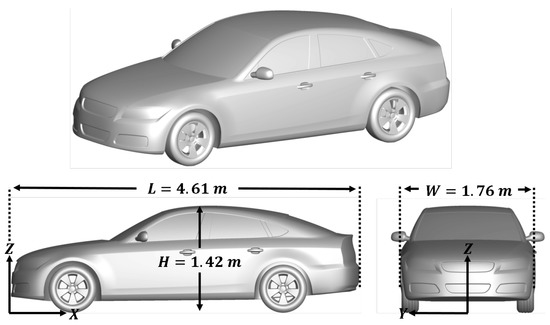
Figure 1.
DrivAer fastback model.
This model has a length (L) of 4.61 m, a width (W) of 1.76 m, a height (H) of 1.42 m, and a wheel base of 2.79 m. For the current work, the smooth underbody was used. The selection of the smooth underbody serves two purposes: it maintains vehicle symmetry for observing the potential bi-stability, and it represents an underbody more aligned with electric vehicles, which are increasingly gaining popularity in the automotive market.
2.2. Domain and Flow Conditions
For the current work, we used the full-scale DrivAer fastback model with a free-stream velocity of 16 m/s. The Reynolds number (based on vehicle length and free-stream velocity) was , and such a Reynolds number matched those from the experiments by Heft et al. [31] and Collin et al. [32], who used a scaled model with a free-stream velocity of 40 m/s. The vehicle model and free-air conditions matched those for the 1st Automotive CFD Prediction Workshop [33]. At the domain inlet (Figure 2), the free-stream velocity was applied with a turbulence intensity of .
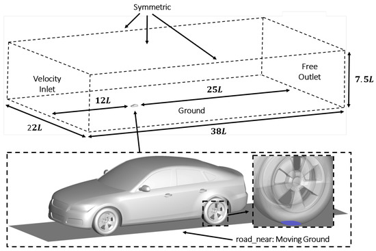
Figure 2.
Computational domain with closeup of moving ground plane (in gray) and morphed tire geometry (in blue) for the rotating wheels case.
The inlet was placed upstream of the vehicle nose, with an outlet positioned downstream of the vehicle base. The vehicle surface was set to a no-slip condition. The surrounding domain walls were set to a symmetry condition to replicate the free-stream, with the exception of the ground plane. For the rotating wheels case, a moving ground condition was applied beneath the vehicle along the ground plane (Figure 2), and the ground plane was set to the free-stream velocity (16 m/s) to replicate the moving belt commonly used in experiments. To simulate the wheel rotation, a sliding mesh condition was used, and a rotational rate of rpm was set in accordance with the free-stream velocity and tire radius. The bottom of the tires intersected the ground plane, creating a morphed geometry. Such morphed geometries resembled the contact patch of a physical vehicle, and such a tire treatment was reported to have good predictive capabilities for flows around the wheels [34,35]. A closeup of the morphed geometry is highlighted in the inset of Figure 2. For the stationary wheels case, a no-slip condition was used both along the ground plane and at the wheels.
2.3. Mesh
Discretization of the domain was performed using the commercial LBM code Power-FLOW (V6-2020). The resultant mesh consists of a lattice of cuboidal elements, referred to as voxels, and the intersection of the voxels with the geometry surface are referred to as surfels. Several refinement regions, called VRs in PowerFLOW, were created near the vehicle surface and wake to capture the relevant wake dynamics. We tested for grid convergence using three grids: coarse, medium, and fine. These grids are visualized through the symmetry and ground planes (Figure 3).
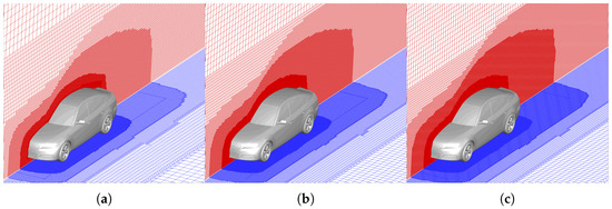
Figure 3.
Meshes used in the current simulations: (a) coarse (89M voxels), (b) medium (174M voxels), (c) fine (272M voxels).
The key parameters of the mesh are summarized in Table 1.

Table 1.
Key mesh parameters in the mesh generation of the vehicle.
2.4. Lattice Boltzmann Method (LBM)
For the current work, LBM simulations are used due to their computational efficiency compared to other methods [30]. LBM has been found to be effective in predicting the wake structure for a variety of vehicle configurations [30,36,37,38]. A thorough review of LBM and its application to automotive flow is described in Kotapati et al. [39] with a summary of the method given as follows.
LBM is based on the Boltzmann equation, which solves for particle motion based on a particle distribution function , where f is the number density of particles at a position x with a speed u at time t. This function can be written in terms of the convective motion of the particles and a collision operator , as in Equation (1).
The collision operator is defined as
where is the time for the velocity distribution function to relax to the equilibrium distribution function . From these equations, the Navier–Stokes and conservation equations can be obtained.
For high Reynolds number flows, PowerFLOW uses a Very Large Eddy Simulation (VLES) approach as a standard practice. The VLES approach directly simulates resolvable scales and models unresolved flow scales using a turbulence model acting as a sub-grid scale (SGS) model. Turbulence modeling is implemented by modifying the relaxation time to yield .
A variant of the RNG equations is used to obtain the turbulent kinetic energy k and turbulent dissipation :
where is the air density, is the stress tensor, and is a dimensionless shear rate. The eddy viscosity in the RNG formulation is represented by the parameter [39].
For the time-marching component of the current simulations, the time-step was automatically calculated by PowerFLOW best-practices criteria. This criteria is based on Equation (6):
where is a proprietary constant (0.236403 for wall-modeled external flow), characteristic length represents the length of the vehicle, resolution is the number of voxels along the vehicle length, and the maximum expected velocity is 1.3 times the free stream velocity. This resulted in three time-step sizes non-dimensionalized by the free stream velocity and vehicle length of ( s), ( s), and ( s) for the coarse, medium, and fine grids, respectively.
For the initial grid convergence study, simulations were carried out over 5.5 s (19 convective time units based on vehicle length and free stream velocity). Time-averaging and statistics were collected over the last 3.0 s (10 convective time units). These simulations were run on the Ohio Supercomputer Center’s (OSC) Owens cluster taking 6,000–17,000 CPU hours depending on mesh density. Additional long-time simulations to capture the bi-stability were carried out on only the coarse mesh using OSC’s Pitzer cluster for 205 s (711 convective time units). Time-averaging and statistics were collected over the last 200 s (694 convective time units). These simulations required roughly 225,000 CPU hours for each wheel condition.
3. Results and Discussion
In this section, results of the computationally efficient LBM simulations for the DrivAer fastback model are reported. The time-averaged flow is first presented and compared with experiments and other well-established computations in Section 3.1 in order to show the validity of the current simulations. The effects of wheel rotation on the long-period (<1 Hz) wake dynamics are discussed next in Section 3.2 by comparing simulation results with and without wheel rotation.
3.1. Time-Averaged Flow
LBM has been found to be accurate for flow predictions around realistic automotive models, comparing well with experiments and other computational methods [30,36,37,38]. We look to compare the forces and the surface pressure to those of experiments and other published simulations to validate the current computational setup. A grid convergence study was performed with a simulation time of s due to the demanding computational expense of the full 200 s simulations. Of this s, the flow field is averaged for the last 3 s. Despite this simulation time being smaller than that used for studying wake bi-stability, the forces and surface pressure fluctuations have achieved adequate time convergence to draw meaningful conclusions.
First, we consider the forces acting on the vehicle. Table 2 compares the coefficients of drag D and lift L using different meshes and wheel conditions. Each force coefficient was calculated as
where A is the frontal area of the vehicle. The vehicle forces match very well with the experimental results [31,32,40]. The coefficient of drag for the rotating wheels case is within of the experimental value for all grids, while an even better match is achieved in the case of stationary wheels. Wheel rotation is found to decrease the total drag acting on the vehicle by relative to the stationary wheels, and such a drag reduction matches well with the experiments of Heft et al. [31]. The small differences in the wheel drag (i.e., the difference in total drag and the vehicle body drag) between the rotating and stationary wheels conditions are consistent with the DES performed by Guilmineau [40]. A lack of difference in wheel drag suggests that very little of the total drag reduction is attributed directly to the drag acting on the wheels. Instead, the change in drag between the rotating and stationary wheels cases is caused by a complex interaction between the wheel flow and the vehicle wake. The wake, characterized as a low-pressure torus, reduces in size over the vehicle base as a result of wheel rotation (Figure 4). Additionally, the lift coefficient also compares well with the experimental results. Only minor variation exists between the coarse and fine grids for both the drag and lift coefficients. The insensitivity of the time-averaged forces on the coarse and fine meshes confirms the adequate resolution of the coarse grid.
Table 2.
Comparison of force coefficients using different meshes and wheel conditions. The subscript denotes the force coefficients attributed directly to the wheels (i.e., the difference in force coefficients between the total vehicle and the vehicle body).
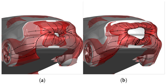
Figure 4.
Iso-surface of the time-averaged total pressure coefficient overlayed with streamlines for the (a) stationary wheels and (b) rotating wheels cases.
Next, we consider the pressure along the symmetry plane of the vehicle surface above and below the wheel axis, dubbed the upper and lower surfaces. The pressure distribution is captured through the pressure coefficient defined as
where is the time-averaged surface pressure, is the free stream pressure, and q is the free stream dynamic pressure . The results were compared to those of the experiments reported in reference [40]. Figure 5 shows that the current simulations effectively replicated the experimental results over both the upper and lower surfaces. Small discrepancies of exist on the upper surface at . However, these features have been attributed to the lack of the mounting strut in the experiments being modeled with the simulations [29,41]. Negligible difference can be observed among the predictions on the fine, medium, and coarse meshes, which further demonstrates grid convergence using the coarse grid.
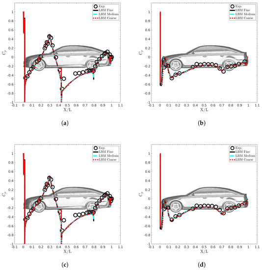
Figure 5.
Comparison of the surface pressure coefficient on the symmetry plane of simulations with experiments [40] on the (a) upper surface (stationary wheels), (b) lower surface (stationary wheels), (c) upper surface (rotating wheels), (d) and lower surface (rotating wheels).
Given the small differences among the solutions across the different grids, grid convergence has been established with the coarse grid. The run on the coarse grid is continued for as long as 200 s to study the wake dynamics, and the wake bi-stability in particular. Further analysis of the grid refinement, including second-order statistics, can be found in Appendix A.
3.2. Long-Period Dynamics
The effects of the long-period wake dynamics are most clearly observed in the time trace of the side-force coefficient (Figure 6). The side-force coefficient was calculated as
where is the instantaneous side force that varies as a function of time t, and (or ) is positive along the positive Y-axis (right side of the vehicle). Large-scale oscillations on the order of 10 s or greater dominate the side force signal for both the stationary and rotating wheels cases. Such long-period oscillations become more apparent in the filtered signals (with a sliding average window of 5 s, corresponding to the peak nausea-inducing frequency of 0.2 Hz or ). Considering that the typical bluff-body vortex shedding periods for the given flow are s (based on a Strouhal number of ), the time periods of these large-scale oscillations are at least one order of magnitude longer than the vortex shedding periods. Such a long-period phenomenon, which is also aperiodic in nature, aligns well with the observations from the side force measurements for the simplified square-back automotive models [2,8], and these previous studies referred to this phenomenon as the bi-stability of the wake. Wheel rotation is found to significantly decrease both the magnitude and periods of these bi-stability oscillations, as evidenced by the peak-to-peak distances highlighted in Figure 6.
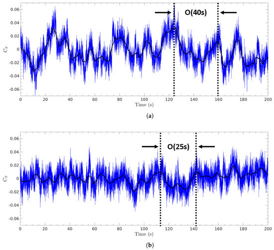
Figure 6.
Time trace of the side-force coefficient for the (a) stationary wheels and (b) rotating wheels cases overlayed with a sliding average using a window size associated with (black).
The impact of wheel rotation on the bi-stability is also apparent when considering the time trace of the surface pressure fluctuations extracted from slices of the upper (), middle (), and lower () regions of the vehicle base (Figure 7). On the upper and middle regions of the base, large low-pressure fluctuations are apparent. These pressure fluctuations show clear asymmetry, switching from one side of the vehicle base to the other intermittently, similar to the oscillations in the side force. Such asymmetric, intermittent switching remains apparent on the lower surface for the stationary wheels case. However, when wheel rotation is applied, the presence of the bi-stability on the lower surface is less clearly distinguishable in comparison to the upper and middle surfaces. Similar to the time traces of the side-force coefficient (Figure 6), the fluctuations of base pressure fluctuations for the rotating wheels case show a shorter time scale compared to the stationary wheels case.
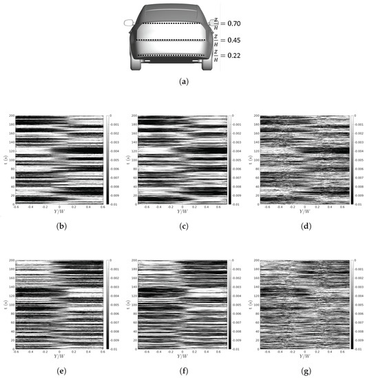
Figure 7.
Fluctuations in the surface pressure coefficient extracted from (a) slices on the vehicle base at (b) (stationary wheels), (c) (stationary wheels), (d) (stationary wheels), (e) (rotating wheels), (f) (rotating wheels), and (g) (rotating wheels).
To visualize the structures pertaining to this bi-stability, we utilize the pressure loss in the wake through iso-surfaces of the instantaneous total pressure coefficient (Figure 8). The total pressure coefficient is defined as
where is the instantaneous total pressure that is the sum of the static pressure P and the dynamic pressure q based on local velocity magnitude, and is the free stream pressure. To best highlight the structures associated with the bi-stable switching, we selected the instantaneous snapshots corresponding to the most positive or negative side forces acting on the vehicle. Similar to the time-averaged flow observed previously, the structures of the wake can be characterized as toroidal in nature. Dynamically, the low-pressure torus is observed to deform similarly to the wake observed for a square-back model [16]. When the side force is positive (right side of the vehicle), the torus predominantly impinges on the right side of the vehicle. While the side force is negative, the torus predominantly impinges on the left side of the vehicle.
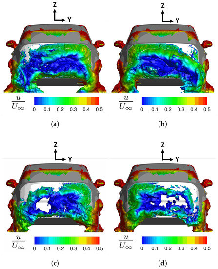
Figure 8.
Iso-surface of the instantaneous total pressure coefficient for the (a) Maximum (stationary wheels), (b) Minimum (stationary wheels), (c) Maximum (rotating wheels), (d) Minimum (rotating wheels). The iso-surfaces are colored by the streamwise velocity to highlight the wake modes.
Although the general wake structure is similar for both cases, wheel rotation directly impacts the structure of the low-pressure torus as switching occurs. In the stationary wheels case, the dominant portion of the low-pressure torus extends across a majority of the vehicle base, and the non-dominant side of the torus deforms, moving away from the vehicle base while maintaining a similar size. In the rotating wheels case, however, the dominant portion of the low-pressure torus envelops less than half of the vehicle base, and the detached portion of the torus shrinks in size. Such a change in size and distortion of the torus may be caused by the increased momentum from the underbody flow when the wheels are set to rotate, as previously observed in the time-averaged wake by Guilmineau [40]. This increased momentum from the underbody displaces the torus farther away from the base surface, weakening the impingement of the wake structure over the base. Decreased impingement by the torus further reduces the pressure loss in the wake during the bi-stable switching for the rotating wheels case. This reduction in pressure loss is consistent with the reduced magnitude of side force oscillations and decreased time period of the switching phenomena when the wheels are rotating, as shown in Figure 6.
The bi-modal nature of the wake is further shown by considering the probability density function (PDF) of the side force (Figure 9). The PDF is calculated based on the filtered time trace with a sliding average window of 5 Hz, similar to the down-sampling used by Perry et al. [8] and Pavia and Passmore [2]. The bi-stability can clearly be discerned from the dual peaks in the PDF. Note that these peaks are asymmetric, which may indicate favorability to one side of the vehicle for the bi-stable switching. A similar asymmetry of the PDF peaks was observed in the experiment of Pavia et al. [4] and was ascribed to the presence of some residual asymmetries in the experimental set-up. Here, we found that the asymmetry of the PDF was caused by the lock of bi-stability into an initial state, the residue of which persisted over long time periods. More than 100 s seems to be required before the development of the second peak that could break the favorability of the initial state, and an even longer signal may be necessary to fully restore the symmetry. The lock of bi-stability into an initial state was also observed in a second independent run on the medium mesh for 50 s (Appendix A), wherein the initial state favored the opposite side of the vehicle, suggesting that the initial state of the bi-stability does not consistently favor one side of the vehicle.
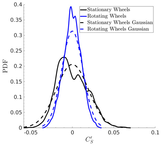
Figure 9.
Probability density function (PDF) of the side-force coefficient filtered at 5 Hz (solid line), in comparison with the PDF of a Gaussian distribution (dashed line).
Although still clearly present in both cases, the bi-stability shows large changes in the side-force PDF when changing the state of the wheels. By using rotating wheels, the PDF becomes thinner, aligning well with the reduction in large-scale fluctuations, as observed in Figure 6. In addition, the two peaks in the PDF of the rotating wheels case have moved closer to each other, resulting in a more symmetric, Gaussian-like profile. Such a trend suggests that the bi-stability becomes less pronounced, albeit still observable, for the rotating wheels case. Additionally, these results also suggest a difference in the bi-stability of the DrivAer model from that of the simplified Windsor model, wherein the implementation of wheels almost fully eliminated a second peak in the PDF of the side force for both stationary and rotating wheel conditions [2].
In order to identify the influence of wheel rotation on the relevant frequencies of the bi-stability, Figure 10 plots the Pre-multiplied Power Spectral Density (PPSD) of the side-force coefficient fluctuations. The PPSD was computed using Welch’s method with a Hamming window, for both stationary and rotating wheels cases. Two window segments were used with an overlap to preserve the low-frequency content. Further increasing the window segments did not change the frequency content for either the stationary or rotating wheels cases.
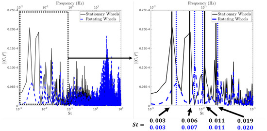
Figure 10.
Pre-multiplied power spectral density (PPSD) of the side-force coefficient for the stationary (black line) and rotating (blue-dashed line) wheels cases.
Both cases capture clear dominant peaks in the frequency band less than 1 Hz (or ). For the stationary wheels case, these dominant frequencies are and . The subharmonics are observed to closely follow the so-called “golden ratio” similar to the turbulent vortex shedding around a cylinder [42] despite not aligning with typical bluff body shedding. In addition, the lowest two frequencies closely align with the peak-to-peak distances observed in the time-trace previously (Figure 6). Similar to the stationary wheels case, nearly identical frequency peaks are captured when implementing rotating wheels. However, a clear reduction in the PPSD is observed in the low-frequency content due to wheel rotation, especially at the lowest frequency of . This reduction in the lowest frequency shows a clear change in the relevant dynamics of the flow around the vehicle when changing the wheel condition, quantifying the changes in side force observed previously (Figure 6 and Figure 9). It should be noted that the dominant side force frequencies from the bi-stability can overlap with the frequency at which the peak motion sickness is induced. For instance, Golding et al. [19] estimated such a motion-sickness frequency to be Hz (), which closely aligns with the dominant frequencies from the bi-stability under the current conditions. We do note that the current study is performed at a relatively low velocity compared to typical highway speeds. Despite this lower velocity, the bi-stable frequency of would still be within the motion-sickness-inducing frequency band (<0.5 Hz) even at typical highway speeds of up to 140 kph [23,24]. Thus, under the current conditions, the bi-stability is associated with lateral oscillations that can induce motion sickness in vehicle occupants.
4. Conclusions
Lattice Boltzmann method (LBM) simulations were performed to study the influence of wheel rotation on the wake dynamics for the realistic DrivAer fastback model. The study found that the wake structure past the vehicle base was characterized as a low-pressure torus. When the wheels were rotating, the size of the low-pressure torus became smaller and less pressure loss occurred within the torus, leading to a reduction in the turbulence intensity in the underbody of the vehicle as well as an overall drag reduction by compared to the stationary wheels case.
Both the time-traces of the side force and pressure fluctuations and the probability density function of the side-force coefficient suggested that the wake bi-stability existed for both the stationary and rotating wheels cases, in which vortex shedding favors one side of the vehicle over the other while maintaining its low-pressure torus structure. When rotating wheels were implemented, the bi-stability became less pronounced with a shorter time scale, and the low-pressure torus displayed an alternating expansion and contraction on the vehicle base instead of an alternating deformation as in the stationary wheels case. For both stationary and rotating wheels cases, the pre-multiplied power spectral density showed that the dominant frequencies of the side force closely aligned with the motion-sickness-inducing frequency, which may suggest that the bi-stability negatively impacts the vehicle occupants for the given DrivAer model and flow conditions.
Author Contributions
Conceptualization, M.A.; methodology, M.A. and R.A.-G.; software, R.A.-G.; validation, M.A.; formal analysis, M.A.; investigation, M.A.; resources, L.D.; data curation, M.A.; writing—original draft preparation, M.A.; writing—review and editing, L.D. and K.D.; visualization, M.A.; supervision, L.D.; project administration, L.D.; funding acquisition, L.D. All authors have read and agreed to the published version of the manuscript.
Funding
The current work was funded under the Strategic Partnership Agreement between The Ohio State University and Honda Development & Manufacturing of America LLC. Computational resources were provided by Ohio Supercomputer Center (OSC) and the Simulation Innovation and Modeling Center (SIM Center).
Acknowledgments
The authors would like to acknowledge the Honda group (Austin Kimbrell, Matt Metka, and Charlie Wilson) for their valuable technical discussions.
Conflicts of Interest
The authors declare no conflict of interest.
Appendix A
Here, further consideration to the grid convergence from Section 3.1 is given through the second-order flow statistics. Figure A1 plots the iso-surfaces of the mean turbulent kinetic energy for both stationary and rotating wheels cases. In both cases, the wake takes on a two-pronged shape, with the highest concentration of k coming from the upper and lower shear layers near the center of the vehicle. When the wheels are stationary, the high concentrations of k extend far beyond the vehicle base from the underbody flow. This underbody turbulence is greatly diminished when the wheels are set to rotate, indicating a heavy influence on the underbody flow. The reduction in the turbulence intensity around the vehicle base is consistent with the smaller size of the low-pressure torus over the vehicle base for the rotating wheels case (Figure 4). Such a trend also suggests an increase in the impact of the underbody flow on the general wake structure due to wheel rotation. Further grid refinement shows little change in the general structure of the turbulent wake. Additionally, Figure A2 further compares the root mean square of the surface pressure fluctuations on the fine, medium, and coarse meshes. Apparent grid convergence is seen among the predictions on the different meshes. As expected, the simulations on all three grids predict high-amplitude pressure fluctuations in regions of large flow separation, including the regions near the A and D pillars and the regions along the center of the rear window and spoiler. These trends match well with the experimental results of Strangfeld et al. [43].

Figure A1.
Iso-surfaces of the turbulent kinetic energy for the (a) coarse (stationary wheels), (b) medium (stationary wheels), (c) fine (stationary wheels), (d) coarse (rotating wheels), (e) medium (rotating wheels), and (f) fine (rotating wheels) meshes.
Figure A1.
Iso-surfaces of the turbulent kinetic energy for the (a) coarse (stationary wheels), (b) medium (stationary wheels), (c) fine (stationary wheels), (d) coarse (rotating wheels), (e) medium (rotating wheels), and (f) fine (rotating wheels) meshes.

In addition to performing the general grid convergence study on the time-averaged flow in Section 3.1, the simulation for the medium mesh was extended to 50 s for the rotating wheels case. Figure A3 shows that the long-period oscillations of the side force are still present regardless of the mesh density. Similarly, the magnitude and time scales associated with these oscillations are comparable between the two meshes. Figure A4 further shows the pressure fluctuations across the base. The bi-stability was still seen on the medium mesh, and little discernible change can be observed between the coarse and medium meshes in the general structure of the bi-stable switching. The insensitivity of the bi-stable switching to grid refinement confirms the adequacy of the baseline coarse mesh for capturing the bi-stability phenomenon.

Figure A2.
Comparison of the root mean square of surface pressure fluctuations for the (a) coarse (stationary wheels), (b) medium (stationary wheels), (c) fine (stationary wheels), (d) coarse (rotating wheels), (e) medium (rotating wheels), and (f) fine (rotating wheels) meshes.
Figure A2.
Comparison of the root mean square of surface pressure fluctuations for the (a) coarse (stationary wheels), (b) medium (stationary wheels), (c) fine (stationary wheels), (d) coarse (rotating wheels), (e) medium (rotating wheels), and (f) fine (rotating wheels) meshes.


Figure A3.
Time-trace of the side-force coefficient for the rotating wheels case on the (a) coarse mesh and (b) medium mesh overlayed with a sliding average using a window size associated with 0.2 Hz (black).
Figure A3.
Time-trace of the side-force coefficient for the rotating wheels case on the (a) coarse mesh and (b) medium mesh overlayed with a sliding average using a window size associated with 0.2 Hz (black).


Figure A4.
Fluctuations in the surface pressure coefficient extracted from (a) slices on the vehicle base at (b) (coarse mesh), (c) (coarse mesh), (d) (coarse mesh), (e) (medium mesh), (f) (medium mesh), and (g) (medium mesh) for the rotating wheels case.
Figure A4.
Fluctuations in the surface pressure coefficient extracted from (a) slices on the vehicle base at (b) (coarse mesh), (c) (coarse mesh), (d) (coarse mesh), (e) (medium mesh), (f) (medium mesh), and (g) (medium mesh) for the rotating wheels case.

References
- Ahmed, S.R.; Ramm, G.; Faltin, G. Some salient features of the time-averaged ground vehicle wake. SAE Trans. 1984, 93, 473–503. [Google Scholar]
- Pavia, G.; Passmore, M. Characterisation of wake bi-stability for a square-back geometry with rotating wheels. In Proceedings of the FKFS Conference, Stuttgart, Germany, 26–27 September 2017; Springer: Cham, Switzerland, 2017; pp. 93–109. [Google Scholar]
- Grandemange, M.; Gohlke, M.; Cadot, O. Turbulent wake past a three-dimensional blunt body. Part 1. Global modes and bi-stability. J. Fluid Mech. 2013, 722, 51–84. [Google Scholar] [CrossRef]
- Pavia, G.; Passmore, M.; Varney, M.; Hodgson, G. Salient three-dimensional features of the turbulent wake of a simplified square-back vehicle. J. Fluid Mech. 2020, 888, A33. [Google Scholar] [CrossRef]
- Pavia, G.; Passmore, M.; Gaylard, A. Influence of Short Rear End Tapers on the Unsteady Base Pressure of a Simplified Ground Vehicle; Technical Report; SAE Technical Paper; SAE: Warrendale, PA, USA, 2016. [Google Scholar]
- Pavia, G.; Passmore, M.; Sardu, C. Evolution of the bi-stable wake of a square-back automotive shape. Exp. Fluids 2018, 59, 20. [Google Scholar] [CrossRef]
- Pavia, G.; Passmore, M.; Varney, M. Low-frequency wake dynamics for a square-back vehicle with side trailing edge tapers. J. Wind Eng. Ind. Aerodyn. 2019, 184, 417–435. [Google Scholar] [CrossRef]
- Perry, A.K.; Pavia, G.; Passmore, M. Influence of short rear end tapers on the wake of a simplified square-back vehicle: Wake topology and rear drag. Exp. Fluids 2016, 57, 1–17. [Google Scholar] [CrossRef]
- Perry, A.K.; Almond, M.; Passmore, M.; Littlewood, R. The study of a bi-stable wake region of a generic squareback vehicle using tomographic PIV. SAE Int. J. Passeng. Cars-Mech. Syst. 2016, 9, 743–753. [Google Scholar] [CrossRef]
- Grandemange, M.; Cadot, O.; Gohlke, M. Reflectional symmetry breaking of the separated flow over three-dimensional bluff bodies. Phys. Rev. E 2012, 86, 035302. [Google Scholar] [CrossRef]
- Grandemange, M.; Gohlke, M.; Cadot, O. Turbulent wake past a three-dimensional blunt body. Part 2. Experimental sensitivity analysis. J. Fluid Mech. 2014, 752, 439–461. [Google Scholar] [CrossRef]
- Brackston, R.D.; De La Cruz, J.G.; Wynn, A.; Rigas, G.; Morrison, J. Stochastic modelling and feedback control of bistability in a turbulent bluff body wake. J. Fluid Mech. 2016, 802, 726–749. [Google Scholar] [CrossRef]
- Evrard, A.; Cadot, O.; Herbert, V.; Ricot, D.; Vigneron, R.; Délery, J. Fluid force and symmetry breaking modes of a 3D bluff body with a base cavity. J. Fluids Struct. 2016, 61, 99–114. [Google Scholar] [CrossRef]
- He, K.; Minelli, G.; Wang, J.; Dong, T.; Gao, G.; Krajnović, S. Numerical investigation of the wake bi-stability behind a notchback Ahmed body. J. Fluid Mech. 2021, 926, A36. [Google Scholar] [CrossRef]
- He, K.; Minelli, G.; Wang, J.; Gao, G.; Krajnović, S. Assessment of LES, IDDES and RANS approaches for prediction of wakes behind notchback road vehicles. J. Wind Eng. Ind. Aerodyn. 2021, 217, 104737. [Google Scholar] [CrossRef]
- Lucas, J.M.; Cadot, O.; Herbert, V.; Parpais, S.; Délery, J. A numerical investigation of the asymmetric wake mode of a squareback Ahmed body–Effect of a base cavity. J. Fluid Mech. 2017, 831, 675–697. [Google Scholar] [CrossRef]
- Varney, M.; Passmore, M.; Gaylard, A. The effect of passive base ventilation on the aerodynamic drag of a generic SUV vehicle. SAE Int. J. Passeng. Cars-Mech. Syst. 2017, 10, 345–357. [Google Scholar] [CrossRef]
- Haffner, Y.; Borée, J.; Spohn, A.; Castelain, T. Mechanics of bluff body drag reduction during transient near-wake reversals. J. Fluid Mech. 2020, 894. [Google Scholar] [CrossRef]
- Golding, J.F.; Mueller, A.; Gresty, M.A. A motion sickness maximum around the 0.2 Hz frequency range of horizontal translational oscillation. Aviat. Space Environ. Med. 2001, 72, 188–192. [Google Scholar] [PubMed]
- Golding, J.F.; Gresty, M.A. Motion sickness. Curr. Opin. Neurol. 2005, 18, 29–34. [Google Scholar] [CrossRef]
- Donohew, B.E.; Griffin, M.J. Motion sickness: Effect of the frequency of lateral oscillation. Aviat. Space Environ. Med. 2004, 75, 649–656. [Google Scholar] [PubMed]
- Young, S. Vehicle NVH development process and technologies. In Proceedings of the 21st International Congress, Beijing, China, 13–17 July 2014. [Google Scholar]
- Bertolini, G.; Straumann, D. Moving in a moving world: A review on vestibular motion sickness. Front. Neurol. 2016, 7, 14. [Google Scholar] [CrossRef] [PubMed]
- Cheung, B.; Nakashima, A. A Review on the Effects of Frequency of Oscillation on Motion Sickness; Defence R&D: Toronto, ON, Canada, 2006. [Google Scholar]
- Grandemange, M.; Cadot, O.; Courbois, A.; Herbert, V.; Ricot, D.; Ruiz, T.; Vigneron, R. A study of wake effects on the drag of Ahmed’s squareback model at the industrial scale. J. Wind Eng. Ind. Aerodyn. 2015, 145, 282–291. [Google Scholar] [CrossRef]
- Sims-Williams, D.; Marwood, D.; Sprot, A. Links between notchback geometry, aerodynamic drag, flow asymmetry and unsteady wake structure. SAE Int. J. Passeng. Cars-Mech. Systems. 2011, 4, 156–165. [Google Scholar] [CrossRef][Green Version]
- Bonnavion, G.; Cadot, O.; Évrard, A.; Herbert, V.; Parpais, S.; Vigneron, R.; Délery, J. On multistabilities of real car’s wake. J. Wind Eng. Ind. Aerodyn. 2017, 164, 22–33. [Google Scholar] [CrossRef]
- Bonnavion, G.; Cadot, O.; Herbert, V.; Parpais, S.; Vigneron, R.; Délery, J. Asymmetry and global instability of real minivans’ wake. J. Wind Eng. Ind. Aerodyn. 2019, 184, 77–89. [Google Scholar] [CrossRef]
- Heft, A.I.; Indinger, T.; Adams, N.A. Experimental and numerical investigation of the DrivAer model. In Fluids Engineering Division Summer Meeting; American Society of Mechanical Engineers: New York, NY, USA, 2012; Volume 44755, pp. 41–51. [Google Scholar]
- Forbes, D.; Page, G.; Passmore, M.; Gaylard, A. A study of computational methods for wake structure and base pressure prediction of a generic SUV model with fixed and rotating wheels. Proc. Inst. Mech. Eng. Part D J. Automob. Eng. 2017, 231, 1222–1238. [Google Scholar] [CrossRef]
- Heft, A.I.; Indinger, T.; Adams, N.A. Introduction of a New Realistic Generic Car Model for Aerodynamic Investigations; Technical Report; SAE Technical Paper; SAE: Warrendale, PA, USA, 2012. [Google Scholar]
- Collin, C.; Mack, S.; Indinger, T.; Mueller, J. A numerical and experimental evaluation of open jet wind tunnel interferences using the DrivAer reference model. SAE Int. J. Passeng. Cars-Mech. Syst. 2016, 9, 657–679. [Google Scholar] [CrossRef]
- 1st Automotive CFD Prediction Workshop. 2019. Available online: https://autocfd.eng.ox.ac.uk/ (accessed on 13 December 2019).
- Ljungskog, E.; Sebben, S.; Broniewicz, A. Inclusion of the physical wind tunnel in vehicle CFD simulations for improved prediction quality. J. Wind Eng. Ind. Aerodyn. 2020, 197, 104055. [Google Scholar] [CrossRef]
- Diasinos, S.; Barber, T.J.; Doig, G. The effects of simplifications on isolated wheel aerodynamics. J. Wind Eng. Ind. Aerodyn. 2015, 146, 90–101. [Google Scholar] [CrossRef]
- Fares, E. Unsteady flow simulation of the Ahmed reference body using a lattice Boltzmann approach. Comput. Fluids 2006, 35, 940–950. [Google Scholar] [CrossRef]
- Islam, A.; Gaylard, A.; Thornber, B. A detailed statistical study of unsteady wake dynamics from automotive bluff bodies. J. Wind Eng. Ind. Aerodyn. 2017, 171, 161–177. [Google Scholar] [CrossRef]
- Aultman, M.T.; Auza-Gutierrez, R.; Wang, Z.; Duan, L. Characterization of the Flow past the Fastback DrivAer Automotive Model Using Unsteady Simulations. In Proceedings of the AIAA Scitech 2021 Forum, Virtual Event, 11–15 & 19–21 January 2021; p. 1329. [Google Scholar]
- Kotapati, R.; Keating, A.; Kandasamy, S.; Duncan, B.; Shock, R.; Chen, H. The Lattice-Boltzmann-VLES Method for Automotive Fluid Dynamics Simulation, a Review; Technical Report; SAE Technical Paper; SAE: Warrendale, PA, USA, 2009. [Google Scholar]
- Guilmineau, E. Numerical simulations of ground simulation for a realistic generic car model. In Fluids Engineering Division Summer Meeting; American Society of Mechanical Engineers: New York, NY, USA, 2014; Volume 46230, p. V01CT17A001. [Google Scholar]
- Peters, B.C.; Uddin, M.; Bain, J.; Curley, A.; Henry, M. Simulating DrivAer with Structured Finite Difference Overset Grids; Technical Report; SAE Technical Paper; SAE: Warrendale, PA, USA, 2015. [Google Scholar]
- Schewe, G. Experimental observation of the “golden section” in flow round a circular cylinder. Phys. Lett. A 1985, 109, 47–50. [Google Scholar] [CrossRef]
- Strangfeld, C.; Wieser, D.; Schmidt, H.J.; Woszidlo, R.; Nayeri, C.; Paschereit, C. Experimental Study of Baseline Flow Characteristics for the Realistic Car Model Drivaer; Technical Report; SAE Technical Paper; SAE: Warrendale, PA, USA, 2013. [Google Scholar]


Publisher’s Note: MDPI stays neutral with regard to jurisdictional claims in published maps and institutional affiliations. |
© 2021 by the authors. Licensee MDPI, Basel, Switzerland. This article is an open access article distributed under the terms and conditions of the Creative Commons Attribution (CC BY) license (https://creativecommons.org/licenses/by/4.0/).