Article

The Influence of the Inter-Relationship of Leg Position and Riding Posture on Cycling Aerodynamics

1
Monash Wind Tunnel Research Platform, Department of Mechanical and Aerospace Engineering, Monash University, Melbourne, VIC 3800, Australia
2
AusCycling, Anna Meares Way, Gepps Cross, SA 5094, Australia
*
Author to whom correspondence should be addressed.
Fluids 2022, 7(1), 18; https://doi.org/10.3390/fluids7010018
Submission received: 15 November 2021 / Revised: 22 December 2021 / Accepted: 23 December 2021 / Published: 31 December 2021
(This article belongs to the Special Issue Aerodynamics of Road Vehicles and Trains)

Abstract

:
Aerodynamics is an important factor affecting cyclist performance, as at the elite level 90% of rider energy is used to overcome aerodynamic drag. As such, much effort has been channeled into understanding the detailed flow around cyclists, since small gains can produce large rewards. Previous studies have shown that cycling aerodynamic drag is sensitive to leg position during the pedaling cycle; however, a systematic analysis comparing the impact of leg position between different riding postures is yet to be undertaken. To address this question, we compare the impact of leg position for two elite-level riding postures: the standard sprint and pursuit body positions. The comparison shows that the effect of leg position on drag is not consistent between the two riding postures, as the altered flow associated with different leg positions is influenced by the wakes from and proximity of other upstream or nearby components, such as the arms. This study reveals the inter-relationship between leg position and riding posture; and suggests that the flow associated with varied leg position should include surrounding geometrical components to obtain and understand the full aerodynamic impact. Practically, the results are valuable for optimizing the posture and improving skin-suit design for drag minimization.

1. Introduction

Aerodynamics is an important factor that contributes to the outcome of many sporting events. Cycling is a good example for which aerodynamics plays an important role in performance, as approximately 90% of a rider’s energy output is used to overcome the aerodynamic drag during competition events [1]. Thus, substantial effort has been channeled to improve rider performance by optimizing the aerodynamic performance. These efforts are generally undertaken from two perspectives: (a) improving the aerodynamic performance of the equipment, and (b) optimizing the rider’s posture for a good balance between ergonomics and aerodynamics.
However, apart from aerodynamically optimizing the geometry of individual bike components and measuring the drag values for different rider configurations, few detailed studies had been undertaken to document the flow structures around a rider-bike system as a whole before Crouch et al. [2] conducted a series of wind-tunnel experiments to systematically characterize the detailed wake structure. Primarily, Crouch et al. [3] characterized the dominant wake structure as a pair of longitudinal trailing vortices, peeling off from the back of the rider and propagating asymmetrically downstream, noting the effect on surface pressure and therefore aerodynamic drag. Griffith et al. [4] conducted numerical simulations based on the rider geometry employed Crouch et al. [3], and indicated that the leg position affects not only the local drag force but also the drag on other body parts, for example, the torso.
After the fundamental work [3,4] of characterizing the flow structures around a rider, much effort has been channeled into advancing our understanding of cycling aerodynamics. For example, research has been extended to understand the aerodynamics of more complex multi-rider configurations, including tandem para-cycling [5], drafting [6] and cycling peloton [7]. Additionally, substantial efforts have been made to understand the correlation between drag and specific rider configurations [8,9,10]. For example, sprint riders in competition always adopt a more aggressive sprint position for a final sprint, for which the torso is lowered to reduce the frontal area and create a more streamlined torso geometry. Based on the wind-tunnel measurements of five sprinting postures of exceptional male and female professional cyclists, Crouch et al. [10] recorded a significant drag reduction for an improved sprint position. At the same time, the authors suggested that most of this reduction was due to changes to the rider’s frontal area. However, repeatability was an issue for such a study in wind-tunnel testing, as it is difficult for an athlete to hold the same posture from one experiment to another. This practical difficulty was overcome by Blocken et al. [9] by basing predictions on numerical simulations. According to these simulations of similar improved sprinting positions, they reported a maximum 24% drag reduction through adopting such positions. Further, they suggested that this benefit was the combined result of a 19% reduction in the frontal area together with a contribution from the altered flow around the cyclist.
A summary of the drag values reported in selected previous literature is provided in Table 1. As shown in previous studies, the aerodynamic performance is sensitive to the rider’s body shape and posture. The results are recorded separately for two common track riding types: sprint and pursuit, although even these can vary from rider to rider. Not surprisingly, a significant variance was recorded from case to case, due to geometric sensitivity. Additionally, most of the fundamental studies on the flow structures and effects of leg positions were conducted only based on the pursuit posture, probably because of its more aerodynamic shape. Furthermore, the conventional approach adopted, both experimentally [3] and numerically [4], for studying the effects of leg position employed mannequins with movable legs. Through this approach, a systematical analysis could be conducted based on a well-defined repeatable geometry; however, such an approach has the limitation of not modeling induced torso/body movement during pedaling, and introduces compromises in the continuity of curvature in key junction areas. Note that these have been shown to have a significant effect [4]. They suggested that future studies based on body position from full scans of real athlete geometries with different leg positions may provide a step towards uncovering the subtle inter-relationship between the flow around different body elements.
Therefore, the current study employs full 3D scans of real athletes at two extreme leg positions to obtain geometries representative of the leg movement over a pedaling cycle. Thus, this study aims to uncouple the aerodynamic effects of leg position on sprint and pursuit riding postures for accurate representative cyclist/bicycle geometries.

2. Methodology

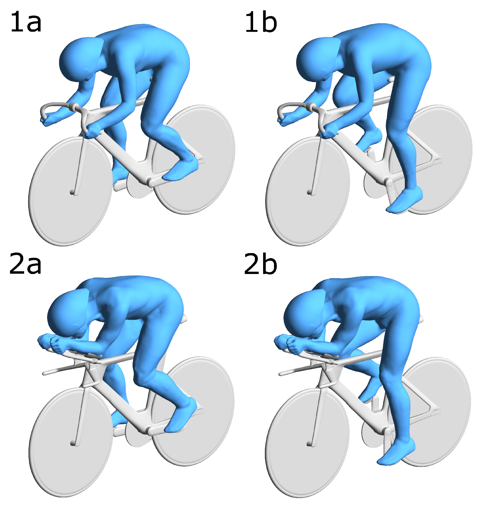
2.1. Geometry and Boundary Conditions

This study was based on 3D scans of two de-identified professional cyclists (subjects 1 and 2) for two leg positions: horizontal (a) and vertical (b), as illustrated in Figure 1. The horizontal position corresponds to the pedals being at the same height while the vertical position indicates the pedals are aligned vertically so that the individual leg positions are the least mirror-symmetric. Of course, conversely, in the horizontal case the upper legs are approximately in the same relative position/alignment although the lower legs are angled differently.
This study does not include optimization of rider posture for aerodynamic efficiency; instead, it aims to characterize the flow field around representative adopted riding postures. Therefore athletes were asked to hold their competition positions during the scan. The work was conducted subject to approval from Monash University’s Human Research Ethics Committee, and written informed-consent documents were collected from the athletes. A suitable competition-level bicycle was acquired from a bike manufacturer. Post scanning, minor simplification, and smoothing were applied to both the rider and bike, for example the surface finish (e.g., skin suit) were not modeled, while all the most aerodynamically important components were maintained.
For the simulations, the rider/bicycle model was positioned at the spanwise center of a hexahedral-element computational domain, as illustrated in Figure 2. In this study, the dimensions are commonly normalized by the typical chord (torso) length (C) of 0.6 m. The computational domain has the size (length:width:height) of 50C: 20C: 17.1C, which gives a blockage ratio of less than 0.5%. The origin of the coordinate system is positioned in the spanwise mid-plane at the crank axis, and x-, y-, z- refers to quantities in the streamwise, spanwise, and vertical directions, respectively. A uniform wind speed of 18 m/s ( U ) with a turbulent intensity level of 5% is applied at the inlet to simulate a typical elite-level competition speed. This gives a Reynolds number of 7.39 × 10 5 based on chord length. A zero-pressure outlet, P s t a t i c = 0 Pa, is utilized far downstream to allow the air to leave the domain freely. The no-slip condition is applied to all rider and bike surfaces. The roughness of the cyclists (e.g., skin suit fabrics) is not modeled in this study; thus, the no-slip boundary condition of zero wall roughness is applied to the cyclist’s surface. The typical value of wall Y+ on the cyclists’ surfaces varies between 5∼40, which is within the recommended range for the selected k ω SST turbulence model [18]. The ground moves at the same speed as the free stream to simulate a relative velocity between the rider and ground, and the corresponding angular velocity of the wheels is calculated. Accordingly, a rotating wall boundary condition with a constant angular velocity ( d θ / d t ) is applied onto the disc wheels and tires. Symmetry boundary conditions are applied to the sides and top of the domain. Specifically, the formulations of the key constraints at the boundaries are presented in Table 2.

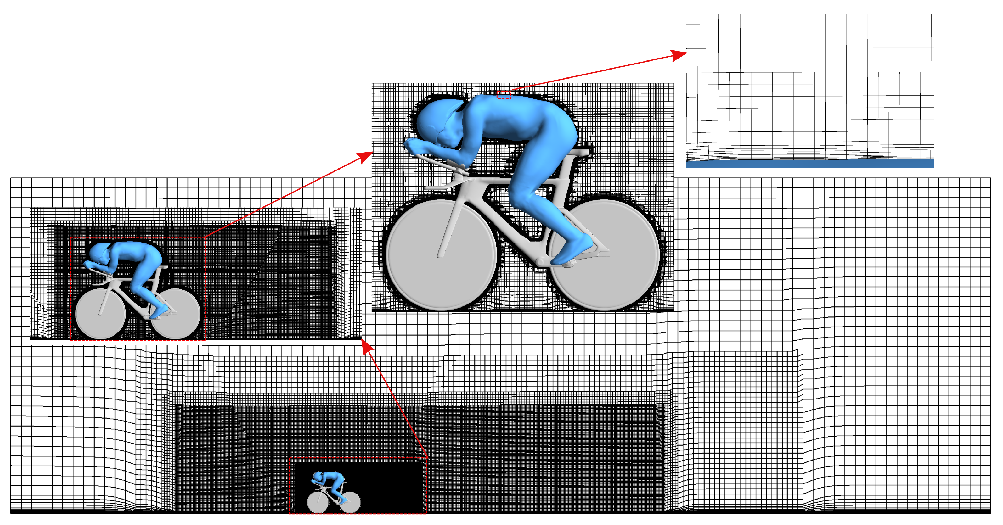
2.2. Meshing Strategy

The overall meshing strategy is based on the predominately Cartesian cut-cell approach, coupled with local mesh refinements around the rider and within the wake. The meshing strategy is illustrated based on the grid layout at the center-plane as shown in Figure 3. In particular, four different levels of refinement are utilized, with the dimensions of the refinement regions determined based on preliminary simulations to ensure that all-important flow features are captured. The typical cell size over the rider/bicycle is 0.002C. Additionally, ten inflation layers with an expansion ratio of 1.2 are typically applied to all wall boundaries to capture the boundary-layer development. Identical meshing parameters were applied to all four cases, with the number of cells approximately 52 million; this number does not change significantly between cases. A coarse mesh of case 1b, obtained by doubling the cell size on the cyclist/model and surrounding field, was constructed to examine grid dependence. The coarse mesh consists of approximately 14.3 million cells. The overall drag prediction shows a reasonably small difference of ∼3% between the two grids, as shown in Table 3. Furthermore, the drag development profiles presented later in Figure 5f imply that the variation is mainly caused by the pressure recovery behind the arms, and a high consistency is achieved elsewhere. Therefore, reasonable grid independence is established, noting the difficulty of further increasing the mesh resolution because of the substantially increased computational cost. Details on deriving the drag development profiles are introduced in Section 3.1.

2.3. Mathematical Model and Solver Description
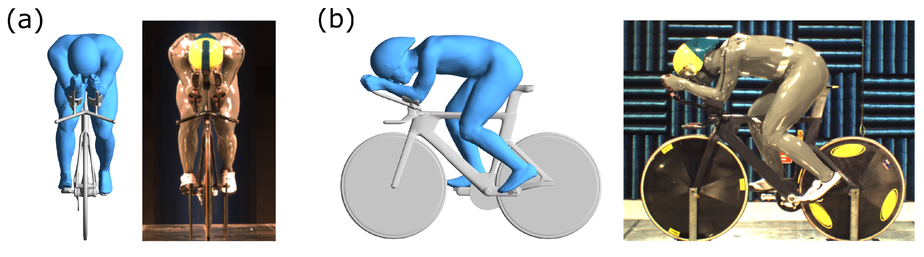
The commercial CFD code FLUENT, which is part of the ANSYS (19.2) software suite, was employed as the numerical flow solver for this study. The pressure-based transient model was adopted to capture the turbulent flow characteristics.
The general simulation procedure is summarised as follows. The flow field was first initialized with a steady-state Reynolds-Averaged Navier-Stokes (RANS) simulation implemented with second-order numerical accuracy. For this, the Shear-Stress Transport (SST) k ω the model was selected as the turbulence model to provide the turbulent viscosity for the RANS equations due to its generally superior performance in modeling the near-wall boundary-layer regions with undefined separation points. A brief discussion of the k ω SST model is presented below, with full details provided in [19].
The model solves transport equations for the turbulent kinetic energy, k, and the specific dissipation, ω :
ρ k t + ρ U i k x i = x i ( μ + σ k μ t ) k x i + P k ˜ β * ρ k ω ,
( ρ ω ) t + ( ρ U i ω ) x i = α ρ S 2 β ρ ω 2 + x i ( μ + σ ω μ t ) ω x i + 2 ( 1 F 1 ) ρ σ ω 2 1 ω k x i ω x i .
Here, ρ is the fluid density, U i is the mean flow velocity component, S is the rate of the strain tensor, P k ˜ are terms associated with turbulence production, and β * , α , β , σ k , σ ω , and σ ω 2 are model constants tuned to give the correct behavior for standard flows. In addition, μ is the molecular viscosity, and μ t = ρ k / ω the turbulent viscosity. Finally, F 1 is a blending function that determines how the equations adjust to resolve the flow as a wall is approached. This is defined by
F 1 = tanh min max k β * ω y , 500 v y 2 ω , 4 ρ σ ω 2 k C D k ω y 2 4 .
Here, y is the distance to the nearest wall, v the wall parallel velocity component and
C D k ω = m a x 2 ρ σ ω 2 1 ω k x i ω x i , 10 20 .
Specifically, as F 1 is varied between 0 and 1, the turbulence model smoothly shifts from the k ϵ model, appropriate away from walls to the k ω model, which is appropriate near walls. As indicated, full details are provided in [19].
Due to the known limitations of the RANS method on predicting turbulent wake flows, especially the behavior of vorticial structures at high Reynolds numbers [20]; therefore, time-dependent simulations were undertaken by switching to the Improved-Delayed Detached Eddy Simulation (IDDES) turbulence model using the RANS-SST solutions as initial fields. This model employs Large-Eddy Simulation (LES) away from walls but blends this with the k ω model near walls to avoid trying to resolve very-fine scale near-wall boundary-layer structures that would otherwise require very fine grid resolution. Switching between these two models is based on a modified length scale d D E S = min ( d , C D E S Δ m a x ) , with d the distance to the closest point on the wall, C D E S an empirical constant (0.65) and Δ m a x the maximum local cell size. Delayed DES (DDES), varies this length scale by adding a shielding function ( f d ) to ensure that LES is not activated within the boundary layer: d D D E S = d f d max ( 0 , d C D E S Δ m a x ) . Finally, Improved DDES (IDDES) introduces the so-called Wall-Modelled LES (WMLES) approach, which allows the outer regions of a boundary layer to be solved using LES when the grid resolution is sufficient, while DDES is employed when it is not. The full details of this model are laid out in the following articles and references [21,22,23], and its implementation in ANSYS-FLUENT is described in [18]. The IDDES model has been widely adopted for modeling related external flows [20].
For convenience, a reference time scale is defined as T ref = C / U , where U is the free-stream velocity. This corresponds to the time taken for the fluid to advect past the rider. The iterative time-stepping scheme is used with up to 20 internal iterations per timestep. Initial testing showed that the predictions are not sensitive to timestep with a timestep of between 0.003 and 0.017 T ref chosen for the simulations reported in this paper. In line with the recommendations for discretization schemes, the second-order upwind scheme was applied to the convective terms in the near-wall RANS (SST- k ω ) turbulence equations, while the bounded central difference scheme was used for the momentum equations, noting the latter suppresses central-difference wiggles that can occur at the high Reynolds number involved.

2.4. Validation

To validate the numerical method and solver settings, the drag predictions are compared with experimental measurements obtained from the Monash University 1.4 MW closed-circuit wind tunnel. The experiments were based on full-scale 3D printed mannequins obtained from the 3D body scans for the pursuit position, as shown in Figure 4. As presented in Table 3, the Drag Area Coefficient ( C D A ) of the combined rider and bike in m 2 for cases 2a and 2b are 0.190 and 0.191, compared to the wind-tunnel values of 0.206 and 0.205. Note that C D A is used because it is directly proportional to the drag force as the frontal area changes. Despite the slight variation in the geometry and boundary conditions (e.g., wind-tunnel tests utilized a splitter plate to remove (most of) the ground boundary layer, while the simulations adopted a moving-ground boundary condition and some small changes/deletions to the geometry), reasonable agreement is achieved between the numerical simulations and wind-tunnel experiments. In this comparison, the drag is under-predicted by approximately 7–8%, while noting that both the simulations and experiments show the little net effect of leg position.

3. Results and Analysis

In this section, the drag areas are firstly compared as a function of riding posture and leg position. To understand the differences in drag, cumulative drag profiles are utilized to demonstrate how the drag is built up along the rider/bicycle, and the drag per unit area distribution on the riders is also visualized. Next, to reveal how different postures and leg positions alter the aerodynamic drag, both the time-averaged and dynamic wake structures are presented and analyzed. The time-averaged wake structure around the rider is first illustrated through an iso-surface of the Q-criterion. Downstream wake evolution is further quantified by examining the flow field at three consecutive downstream locations behind the rider. In addition, the wake’s turbulence level is calculated, and the dominant larger-scale dynamic features extracted.

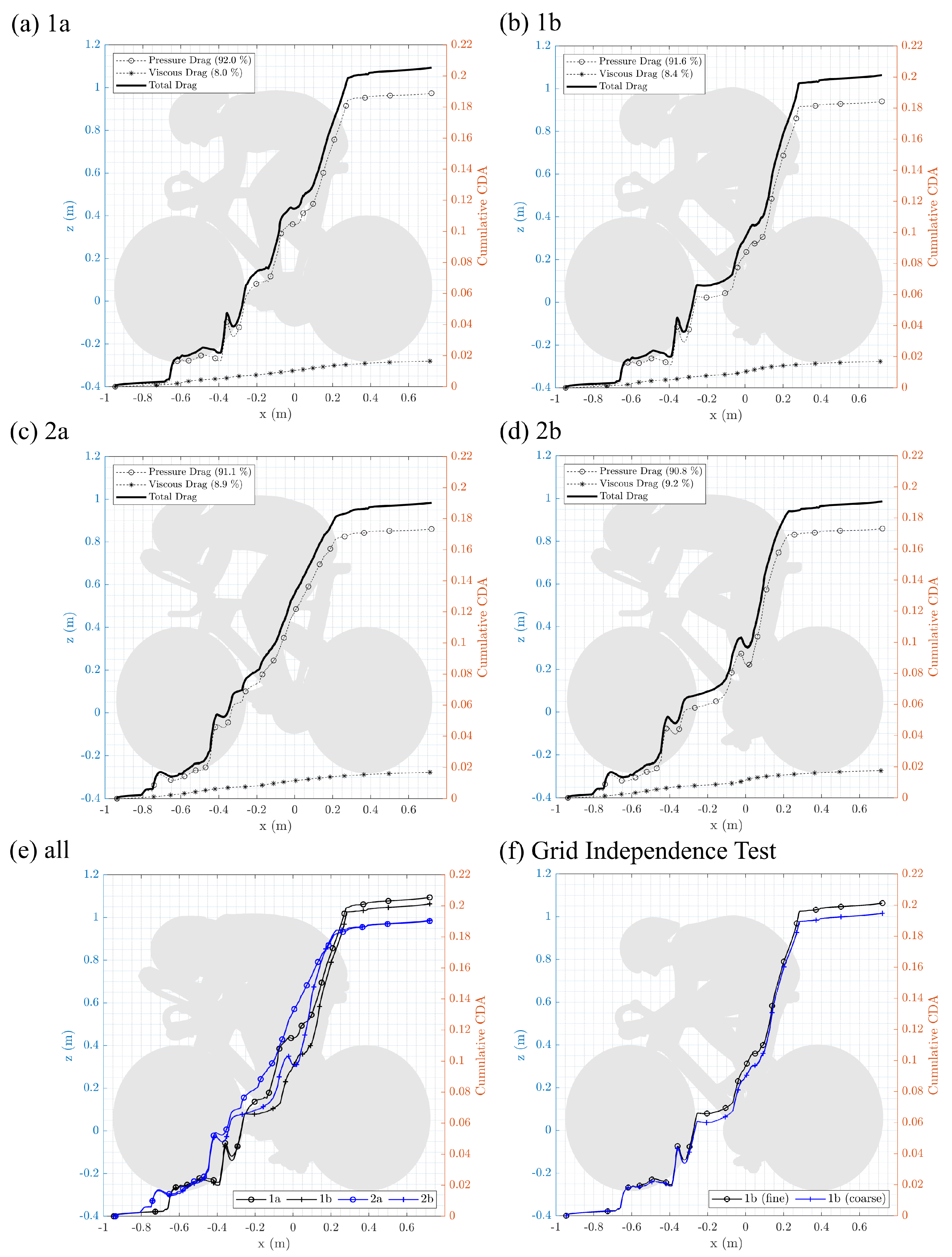
3.1. Aerodynamic Loading

To begin with, C D A s is compared across the four variations of riding posture and leg position. Here, C D A is the Drag Area Coefficient of the rider and bike combination measured in m 2 , and the corresponding drag coefficients ( C D ) are calculated based on the frontal areas, which are also listed in Table 3. According to Table 3, the pursuit positions generally show a smaller C D A than the sprint positions, while if we take the frontal area into account, the difference in C D becomes less significant. The mean C D A s of cases 1a, 1b, 2a and 2b are 0.205, 0.201, 0.190 and 0.191, respectively, as presented in Table 3. Perhaps surprisingly, for both riding types, C D A was not found to vary significantly with leg position in this study, compared to a previous experimental study of Crouch et al. [3] for an idealized mannequin. However, this relative insensitivity to leg position is consistent with more recent wind-tunnel measurements of 0.206 and 0.205 for cases 2a and 2b. At this stage, the cause of the reduced impact of leg position for these two postures compared to that for the previous study of Crouch et al. [3] for a mannequin (∼10–15%) is unknown, but is likely due to the significantly more-upright posture of that study and slighter body type. This requires further investigation.
Cumulative drag profiles are utilized to depict how the overall drag is built up as the air passes the rider/bicycle. The cumulative drag of individual cases is presented in Figure 5a–d, with silhouettes overlapped for location referencing. The contribution of pressure and viscous force to the overall drag for each case is also calculated and plotted in the corresponding subfigures. According to Figure 5a–d, the accumulated viscous drag increases steadily along the body surface at a rate approximately proportional to the surface area. Additionally, the total viscous drag is consistent between the 4 cases, which accounts for about 8–9% of the total drag.
The cumulative drag profiles of all cases are plotted in Figure 5e to enable a direct comparison. According to Figure 5e, although the difference in overall drag between the leg positions is minor, the way drag develops along the model is identifiably different. In general, the outstretched legs in a vertical leg position delay the occurrence of rapid drag increase, and the dropped arms in the sprint posture delay the occurrence of a local drag peak. Overall, Figure 5 indicates that the effects of leg and arm positions on the aerodynamic loading are coupled.
To further demonstrate this, the drag per unit area distribution over the rider surface is illustrated in Figure 6 to visualize the correlation between posture and drag contributions. The local drag shown in Figure 6 is calculated by integrating the pressure and skin friction in the streamwise direction over the surface mesh. Red represents drag in the same direction as the freestream, while blue represents thrust in the direction opposite the free-stream. Local flow separation at the edges of the bluff body parts (e.g., arms and legs) causes these negative drag (blue) regions. According to Figure 6, the main sources of drag are (1) direct flow impingement on the windward area; and (2) the pressure drag induced from the separated flow at the back of the riders. The drag on the extended legs increases because more body surface is exposed to the incoming flow, while the drag on the thighs of the raised legs is reduced as they are more aligned with the free stream. Additionally, the raised leg significantly increases the drag on the torso for the sprint rider, while this effect is not obvious for the pursuit rider. This is because the wider arms in the sprint posture allow more air intake between the arms, and the flow accelerates over the torso as the raised leg reduces the gap. As a result, the viscous drag on the torso increases. In comparison, the closed arms in the pursuit posture effectively block the incoming wind from passing over the torso; hence the impact of the adjacent thighs on the torso is not as significant. From a practical viewpoint, understanding the drag distribution over-riders is valuable for optimizing the posture and improving the skin-suit design to modify both flow separation and the downstream flow to assist with drag minimisation.

3.2. Dominant Wake Flow Structures

The dominant vortical flow structures around the riders are visualized using an iso-surface of the Q-criterion (Q = 1000 1/s 2 ) and coloured by the mean longitudinal vorticity ( ω x ¯ ), as shown in Figure 7. Despite the wake’s turbulent nature, some persistent streamwise vortical structures, including the vortices generated from the helmet, shoulders, arms, torsos, hips, legs, and shoes, are captured. In general, straightening the leg switches its wake from being dominated by longitudinal vortices to separation-dominated. Additionally, the diagonal vortex pair formed behind the back and hip is dragged towards the low-pressure region formed behind the outstretched leg, increasing the asymmetry of the wake. This is the underlying reason why the wakes behind vertical leg positions are more asymmetric than those behind the horizontal leg positions, as has been previously reported in the literature [3].
Persistent streamwise vortices are formed at the upper arms and roll off from the shoulders of both riding postures, with the arm positions significantly influencing their appearance. Specifically, the vortices are more attached to the torso with the arms closed in the pursuit posture. In comparison, the open arms of the sprint posture allow more air intake between the arms, and a higher momentum flux onto the chest and around the hips, magnifying the flow alteration due to the leg positioning. This is consistent with the drag per unit area distribution over the torsos, as shown in Section 3.1. Additionally, Figure 7 also illustrates some persistent streamwise vortical structures that are not sensitive to the leg position or riding posture, for example, the streamwise vortices originating from the helmet and ankles.

3.3. Wake Propagation

According to the wake structure revealed in Section 3.2 above, the wake behind a rider is highly three-dimensional with a mixed range of scales. The downstream evolution of time-averaged wake structure is visualized by x-vorticity (streamwise) and in-surface projected velocity vectors on three consecutive vertical planes at 0.5, 1, and 2C from the back of rider, as presented in Figure 8. The boundaries of the vorticity-dominated regions are captured by iso-lines of Γ 2 = 2 / π , and the location of vortex cores are calculated based on the local minimum of Γ 1 , noting this is a common vortex identification method adopted by experimentalists [24] to identify rotation-dominated regions and vortex core centers. Figure 8 illustrates the evolution of the time-averaged trailing vortex structure as it advects downstream. In general, the diagonal vortices originating from the hip and back are the dominant wake structures for all cases, except for 2a for which the structure from the right shoulder is more dominant. Comparing the wake behind the two riding postures, the open arms in the sprint posture widen the wake, while the vortices from the shoulders are more predominant in the pursuit posture. The tendency of introducing asymmetry to the wake by positioning the legs vertically, as reported from previous studies [3], is more profound on the pursuit posture. The asymmetry effect is mainly caused by the unbalanced pressure introduced by the legs, specifically, the larger low-pressure region behind the outstretched leg drags the surrounding wake structures towards it. Therefore, a possible explanation is that the open arms of a sprint cyclist create a larger and more turbulent wake region, which weakens the significance of the local low-pressure region caused by the outstretched leg.
From these sequences, ω x ¯ at the cores of the primary (hip) longitudinal vortices is utilized to quantify the strength and the decay of the wake as it advects from 0.5 to 2C behind the rider, as plotted in Figure 9. According to this figure, the decay rate of the primary trailing vortex is significantly different between the sprint and pursuit postures. The trailing vortex peeling from the sprint rider initially has higher strength; however, its magnitude drops rapidly within the near-wake region due to the higher turbulence caused by the open arms. In comparison, the vortex behind the pursuit rider decays at a slower and more steady rate. Additionally, the strength of the trailing vortex associated with horizontal leg positions is generally higher than that associated with vertical leg positions. The strength of trailing vortices is closely correlated with aerodynamic drag, as energy has to be channeled to form these persistent structures. This can partially explain why with more separation and asymmetry caused by the outstretched leg, the difference in overall drag value between the leg positions is not significant. Therefore, correctly resolving the entire flow field is key to revealing the sources of aerodynamic drag.

3.4. Wake Dynamics

The wake dynamic response is analyzed based on the velocity field at 1 C behind the rider, and results are presented in Figure 10. The time-averaged velocity and turbulence intensity ( T I ( % ) ) are respectively presented in the first two columns in Figure 10. Consistent with the flow field shown in Section 3.2 and Section 3.3, the wake of sprint cyclist is wider and more turbulent. Additionally, Proper Orthogonal Decomposition (POD) is employed to extract the most energetic features (modes) contributing to the wake flow. Specifically, by calculating the optimal orthogonal basis (modes) of a time sequence of wake states ordered by energy content, coherent dynamic features from a turbulent (i.e., unsteady) flow field is extracted. This study utilizes the snapshot POD method, which was introduced by Sirovich [25], and has been extensively used to provide insight into complex flow fields [26]. POD is implemented on the velocity magnitude field at 1 C behind the rider, and the structure of the first three most energetic modes are plotted in columns 3–5 in Figure 10, with the associated energy percentage printed at the top right corner. Note that the sign of the modes in Figure 10 is arbitrary so that the first mode for all cases is essentially identical. The consistency of mode 1 implies that the primary dynamic feature for all the cases, regardless of leg positions and riding postures, is wake speed variation around the left thigh/hip. The second mode for the vertical leg cases indicates a vertical energy fluctuation at the same location, as shown in column 2, while this feature is not apparent with horizontal legs. This presumably corresponds to a vertical fluctuation in the position of the streamwise vortical structure observed in the time-mean wake. Interestingly, this mode is not one component of a mode pair (separated by 90 in-phase), suggesting that the fluctuations are not quasi-periodic. Additionally, the energy percentages of the first modes indicate that energy pulsing is more dominant with the legs horizontal. In contrast, with the legs positioned vertically, some energy is redirected to energize the vertical fluctuation. Beyond mode 3, the spatial distributions don’t show clear features, which indicates the chaotic nature of the near wake. Increasing the length of the dataset for extracting the POD modes may improve the convergence of higher-order modes; however, given the practical limitation imposed by already substantial computational expense, it is difficult to justify an increased sampling time to better resolve those modes, especially for a highly chaotic flow field with mixed turbulent time and length scales.

4. Conclusions

In this study, the effects of leg position on aerodynamic loading for two competition sprints and pursuit cyclists with different postures have been investigated. Although the overall drag for each leg position is similar for each posture, the force distribution and flow over the cyclist’s body vary significantly for the different postures. Specifically, the impacts of leg and arm positions on cycling aerodynamics are strongly coupled. In particular, raised legs to increase the friction drag on the torso, and this effect is found to be stronger with dropped arms (i.e., the sprint posture). This is because the widely-placed arms in the sprint posture allow more high-speed air to travel through the gap between the torso and raised leg, which makes the blockage effect of the raised leg more profound. In addition, by exposing widely placed arms to the free stream, the wake behind the sprint rider is widened, and the level of turbulence is amplified. Furthermore, the higher wake turbulence level of the sprint posture increases the decay rate of trailing streamwise vortices within the near-wake region, while weakening the asymmetry effect seen on the trailing vortices and introduced by the low-pressure region behind the outstretched leg. In comparison, the closed arms in the pursuit posture effectively block the air intake towards the torso, reducing the overall effect of varying leg position. Finally, the low-pressure region created behind the outstretched leg enhances wake asymmetry by dragging the trailing vortices from the back and hip towards it.
Therefore, the impacts of leg positions vary between different riding postures due to the strong interaction between the flow structures from different body parts. Thus, this study suggests that investigations into the effects of leg position need to include representative human geometries because of complex flow interactions. Indeed, obtaining an accurate cyclist/bicycle geometry is critical as the overall flow field is found to be highly geometry dependent, and conclusions may not be generalizable. As a final remark to reinforce this point, it is worth reiterating that the experimental study of Crouch et al. [3] showed a ∼10–15% difference in aerodynamic drag for the horizontal and vertical leg positions, while for the more compact sprint and pursuit postures considered here, no discernible difference could be detected.

Author Contributions

Conceptualization, S.W. and J.P.; Data curation, S.W.; Investigation, S.W.; Methodology, S.W.; Project administration, D.B., M.C.T. and T.C.; Resources, J.P.; Software, S.W.; Supervision, M.C.T. and D.B.; Validation, S.W., D.T.S. and C.B.; Visualization, S.W.; Writing—original draft, S.W.; Writing—review & editing, J.P., M.C.T. and D.B. All authors have read and agreed to the published version of the manuscript.

Funding

This research was funded by the Australian Institute of Sport.

Institutional Review Board Statement

Not applicable.

Informed Consent Statement

Informed consent was obtained from all subjects involved in the study.

Data Availability Statement

Data are available upon request to the authors under confidentiality agreement.

Conflicts of Interest

The authors declare no conflict of interest.

References

  1. Kyle, C.; Weaver, M. Aerodynamics of human-powered vehicles. Proc. Inst. Mech. Eng. Part A J. Power Energy 2004, 218, 141–154. [Google Scholar] [CrossRef]
  2. Crouch, T.; Thompson, M.; Burton, D.; Sheridan, J.; Brown, N. Dominant flow structures in the wake of a cyclist. In Proceedings of the 30th AIAA Applied Aerodynamics Conference, New Orleans, LA, USA, 25–28 June 2012; p. 3212. [Google Scholar]
  3. Crouch, T.N.; Burton, D.; Brown, N.A.T.; Thompson, M.C.; Sheridan, J. Flow topology in the wake of a cyclist and its effect on aerodynamic drag. J. Fluid Mech. 2014, 748, 5–35. [Google Scholar] [CrossRef]
  4. Griffith, M.D.; Crouch, T.; Thompson, M.C.; Burton, D.; Sheridan, J.; Brown, N.A. Computational fluid dynamics study of the effect of leg position on cyclist aerodynamic drag. J. Fluids Eng. 2014, 136, 101105. [Google Scholar] [CrossRef] [Green Version]
  5. Mannion, P.; Toparlar, Y.; Blocken, B.; Clifford, E.; Andrianne, T.; Hajdukiewicz, M. Aerodynamic drag in competitive tandem para-cycling: Road race versus time-trial positions. J. Wind Eng. Ind. Aerodyn. 2018, 179, 92–101. [Google Scholar] [CrossRef]
  6. Blocken, B.; Toparlar, Y.; van Druenen, T.; Andrianne, T. Aerodynamic drag in cycling team time trials. J. Wind Eng. Ind. Aerodyn. 2018, 182, 128–145. [Google Scholar] [CrossRef]
  7. Blocken, B.; van Druenen, T.; Toparlar, Y.; Malizia, F.; Mannion, P.; Andrianne, T.; Marchal, T.; Maas, G.J.; Diepens, J. Aerodynamic drag in cycling pelotons: New insights by CFD simulation and wind tunnel testing. J. Wind Eng. Ind. Aerodyn. 2018, 179, 319–337. [Google Scholar] [CrossRef]
  8. Barry, N.; Burton, D.; Sheridan, J.; Thompson, M.; Brown, N.A. Aerodynamic performance and riding posture in road cycling and triathlon. Proc. Inst. Mech. Eng. Part P J. Sport. Eng. Technol. 2015, 229, 28–38. [Google Scholar] [CrossRef]
  9. Blocken, B.; van Druenen, T.; Toparlar, Y.; Andrianne, T. CFD analysis of an exceptional cyclist sprint position. Sport. Eng. 2019, 22, 10. [Google Scholar] [CrossRef] [Green Version]
  10. Crouch, T.; Menaspà, P.; Barry, N.; Brown, N.; Thompson, M.C.; Burton, D. A wind-tunnel case study: Increasing road cycling velocity by adopting an aerodynamically improved sprint position. Proc. Inst. Mech. Eng. Part J. Sport. Eng. Technol. 2019, 235. [Google Scholar] [CrossRef]
  11. Fintelman, D.; Sterling, M.; Hemida, H.; Li, F.X. The effect of crosswinds on cyclists: An experimental study. Procedia Eng. 2014, 72, 720–725. [Google Scholar] [CrossRef]
  12. Jeukendrup, A.E.; Martin, J. Improving cycling performance. Sport. Med. 2001, 31, 559–569. [Google Scholar] [CrossRef]
  13. Defraeye, T.; Blocken, B.; Koninckx, E.; Hespel, P.; Carmeliet, J. Aerodynamic study of different cyclist positions: CFD analysis and full-scale wind-tunnel tests. J. Biomech. 2010, 43, 1262–1268. [Google Scholar] [CrossRef] [Green Version]
  14. Griffith, M.D.; Crouch, T.N.; Burton, D.; Sheridan, J.; Brown, N.A.; Thompson, M.C. A numerical model for the time-dependent wake of a pedalling cyclist. Proc. Inst. Mech. Eng. Part P J. Sport. Eng. Technol. 2019, 233, 514–525. [Google Scholar] [CrossRef]
  15. García-López, J.; Rodríguez-Marroyo, J.A.; Juneau, C.E.; Peleteiro, J.; Martínez, A.C.; Villa, J.G. Reference values and improvement of aerodynamic drag in professional cyclists. J. Sport. Sci. 2008, 26, 277–286. [Google Scholar] [CrossRef]
  16. Underwood, L.; Schumacher, J.; Burette-Pommay, J.; Jermy, M. Aerodynamic drag and biomechanical power of a track cyclist as a function of shoulder and torso angles. Sport. Eng. 2011, 14, 147–154. [Google Scholar] [CrossRef]
  17. Barry, N.; Burton, D.; Sheridan, J.; Thompson, M.; Brown, N.A. Aerodynamic drag interactions between cyclists in a team pursuit. Sport. Eng. 2015, 18, 93–103. [Google Scholar] [CrossRef]
  18. Ansys, A.F. 14.0 Theory Guide; ANSYS Inc.: Canonsburg, PA, USA, 2011; Volume 390, p. 732. [Google Scholar]
  19. Menter, F.R.; Kuntz, M.; Langtry, R. Ten years of industrial experience with the SST turbulence model. Turbul. Heat Mass Transf. 2003, 4, 625–632. [Google Scholar]
  20. Wang, S.; Bell, J.R.; Burton, D.; Herbst, A.H.; Sheridan, J.; Thompson, M.C. The performance of different turbulence models (URANS, SAS and DES) for predicting high-speed train slipstream. J. Wind Eng. Ind. Aerodyn. 2017, 165, 46–57. [Google Scholar] [CrossRef]
  21. Shur, M.L.; Spalart, P.R.; Strelets, M.K.; Travin, A.K. A hybrid RANS-LES approach with delayed-DES and wall-modelled LES capabilities. Int. J. Heat Fluid Flow 2008, 29, 1638–1649. [Google Scholar] [CrossRef]
  22. Gritskevich, M.S.; Garbaruk, A.V.; Schütze, J.; Menter, F.R. Development of DDES and IDDES formulations for the k-ω shear stress transport model. Flow, Turbul. Combust. 2012, 88, 431–449. [Google Scholar] [CrossRef]
  23. Saini, R.; Karimi, N.; Duan, L.; Sadiki, A.; Mehdizadeh, A. Effects of near wall modeling in the improved-delayed-detached-eddy-simulation (IDDES) methodology. Entropy 2018, 20, 771. [Google Scholar] [CrossRef] [PubMed] [Green Version]
  24. Graftieaux, L.; Michard, M.; Grosjean, N. Combining PIV, POD and vortex identification algorithms for the study of unsteady turbulent swirling flows. Meas. Sci. Technol. 2001, 12, 1422. [Google Scholar] [CrossRef]
  25. Sirovich, L. Turbulence and the dynamics of coherent structures. I. Coherent structures. Q. Appl. Math. 1987, 45, 561–571. [Google Scholar] [CrossRef] [Green Version]
  26. Wang, S.; Avadiar, T.; Thompson, M.C.; Burton, D. Effect of moving ground on the aerodynamics of a generic automotive model: The DrivAer-Estate. J. Wind Eng. Ind. Aerodyn. 2019, 195, 104000. [Google Scholar] [CrossRef]
Figure 1. Illustration of CFD rider/bicycle geometries: 1a,1b and 2a,2b represent sprint (top row) and pursuit (bottom row) postures with horizontal (left column) and vertical (right column) leg positions respectively.
Fluids 07 00018 g001
Figure 2. Schematic of the numerical domain showing dimensions and boundary settings.
Fluids 07 00018 g002
Figure 3. Meshing strategy and local refinement illustrated by the grid of case 2a through the centre-plane.
Fluids 07 00018 g003
Figure 4. Comparison between the front-on (a) and side-on (b) CFD and wind-tunnel geometries based on the case 2a.
Fluids 07 00018 g004
Figure 5. Cumulative (pressure and skin friction) drag profiles across the rider/bicycle with streamwise distance: (a) 1a, (b) 1b, (c) 2a, (d) 2b, (e) all 4 cases, (f) 1b with fine and coarse grids.
Fluids 07 00018 g005
Figure 6. Comparison of local drag per unit area distribution over the riders: (a) isometric view from the front; (b) isometric view from the back.
Fluids 07 00018 g006
Figure 7. The dominant time-mean vortical flow structures around the rider visualised by the iso-surface of Q-criterion and coloured by the longitudinal vorticity ( ω x ¯ ).
Fluids 07 00018 g007
Figure 8. The wake propagation depicted by ω x ¯ and in-surface projected velocity vectors at 0.5, 1 and 2C behind the cyclist, with the boundaries of dominant vortices visualized by green lines and their core location highlighted by green crosses (x). The outlines of the cyclist and bicycle are plotted to show the relative position between the wake and cyclists.
Fluids 07 00018 g008
Figure 9. A quantitative comparison of the wake decay based on ω x ¯ at the vortex cores varying from 0.5 to 2 C behind the rider.
Fluids 07 00018 g009
Figure 10. The wake dynamics presented by the time-averaged velocity (column 1), turbulence intensity (column 2), and the structure of first three most energetic modes (column 3∼5) at 1 C behind the back of the cyclist. The outlines of the cyclist and bicycle are also plotted here to show the relative position between the wake and cyclists.
Fluids 07 00018 g010
Table 1. Drag measurements/predictions from previous studies.
CaseFrontal Area
(m 2 )
Leg PositionMethod C D A
(m 2 )
Sprint[9]0.37horizontalCFD0.236
[5]0.3979horizontalCFD0.233
[11]NAhorizontalWT0.3
[8]0.4594dynamicsWT0.306
[12]NAdynamicsWT0.307
[13]NAhorizontalWT0.243
Pursuit[5]0.3935horizontalCFD0.213
[4]NAhorizontalCFD0.201
(from plots)
[4]NAverticalCFD0.166
(from plots)
[14]NAhorizontal
(dynamics)
CFD0.15
(from plots)
[14]NAvertical
(dynamics)
CFD0.19
(from plots)
[8]0.3855dynamicsWT0.283
[12]NAdynamicsWT0.259
[15]NAhorizontalWT0.26
[16]NAdynamicsWT0.26∼0.296
[13]NAhorizontalWT0.211
[17]NAdynamicsWT0.214∼0.251
Table 2. Expressions of the constraints at the domain boundaries. Note the subscripts of n o r m a l and t a n g e n t i a l refer to the quantities in the normal and tangential direction of the boundaries, R w h e e l refers to the radius of the wheels.
Boundary LocationsBoundary TypesExpressions of Constraints
InletVelocity inlet U x = U , U y , z = 0
OutletPressure outlet P s t a t i c = 0
Top and SidesSymmetry U n o r m a l = 0 , P n o r m a l = 0
GroundMoving wall (translation) U x = U , Y y , z = 0
Rider and bike frameStationary wall U t a n g e n t i a l = 0
Bike wheels and tyresMoving wall (rotation) d θ / d t = U / R w h e e l
Table 3. The comparison of drag predictions.
1a1b1b (Coarse)2a2b
Frontal Area (m 2 )0.3670.3700.3700.3520.351
C D A mean0.2050.2010.1950.1900.191
std0.0060.0040.0040.0040.003
C D mean0.5600.5440.5270.5400.543
std0.0150.0110.0110.0110.009
C D A (Wind Tunnel) 0.2060.205
Publisher’s Note: MDPI stays neutral with regard to jurisdictional claims in published maps and institutional affiliations.

